Software Reliability Measurements in N-Version ... - Semantic Scholar

Software Reliability Measurements in N-Version Software Execution Environment

Michael R. Lyu Bellcore Information Sciences and Technologies Research Lab. Morristown, NJ 07962 (319)335-5957 Abstract N -Version Programming has been proposed as a means to increasing software reliability by the attributes provided in fault tolerance. In this paper we will quantitatively examine the effectiveness of this approach. We look into the details of an academia/industry joint project employing six programming languages, and study the properties of the resulting program versions. We explain how exhaustive testing was applied to the project, and measure the error probability in different N -Version Software execution configurations. To explore the manifestations of errors resulting from each programming fault, and to study their impact to N -Version Software systems, we apply mutation testing techniques to gain more insights. We further define several reliability-related quantities, including error frequency function, error severity function, error similarity function, and safety coverage factor. With the multiple program versions obtained in the project, we create a total of 93 mutants, and measure the reliability quantities for each of them. Based on these quantities, we estimate the safety coverage factor for the N-Version Software system, which reveals the potential of this technique in improving software reliability. A side observation of this research is that the per fault error rate does not remain constant in this computation-intensive project. The error rates associated with each program fault differ from each other dramatically. However, they tend to decrease as testing progresses. This information might be helpful for practitioners to decide which models to apply for software reliability measurement in a similar project. Keywords: Software Failure Data, N-Version Programming, Mutation Testing, Software Reliability, Coverage Analysis.

-1-

Software Reliability Measurements In N-Version Software Environment

1. Introduction The N -Version Programming (NVP) approach to fault-tolerant software systems involves the generation of functionally equivalent, yet independently developed software components, called N -version software (NVS)[1]. These components are executed concurrently under a supervisory system that uses a decision algorithm based on consensus to determine final output values[2]. Whenever probability of similar errors is minimized, distinct, erroneous results tend to be masked by a majority vote during NVS execution[3]. NVS systems are gaining acceptance in critical application areas such as the aerospace industry[4] [5] [6] [7], nuclear power industry[8] [9] [10], and ground transportation industry[11] [12]. However, the evaluations of such systems, especially in the context of reliability-related measures, are still left as a controversial issue. There are many conflicting observations about the effectiveness of this fault-tolerance technique in increasing software reliability[13] [14]. In this paper, we will revisit the program versions obtained in a six-language project, using Ada, C, Modula-2, Pascal, Prolog, and T (a lisp dialect)[15], and evaluate the reliability aspects of the resulting NVS executions from various angles.

2. The Automatic Landing Problem An industrial investigation concerning the effectiveness of the NVP process was conducted in an academia/industry joint project utilizing an NVP design paradigm[16]. The application was an automatic flight control function for the landing of commercial airliners that had been implemented by the Honeywell Incorporated to build a 3-version Demonstrator System (hardware and software), employed to show the feasibility of N-version programming for this type of application. The specification could be used to develop the software of a flight control computer (FCC, or autopilot) for a real aircraft, given that it was adjusted to the performance parameters of a specific aircraft. All algorithms and control laws in the application were specified by diagrams

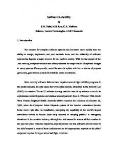
-2which had been certified by the Federal Aviation Administration (FAA). The pitch control part of the automatic landing problem, i.e., the control of the vertical motion of the aircraft, was selected for the project. The major system functions of the pitch control and its data flow are shown in Figure 1. hhhhhhhhhhhhhhhh

hhhhhhhhhhhhhhhh

c

c c BAROMETRIC c I x ALTITUDE c ALTITUDE chc hhhhhhhhhhhhhhhhhhhhhhhhhhhhhhhhhc c c HOLD hhhhhhhhc COMP. FILTER c chhhhhhhhhhhhhhhh c hhhhhhhhhhhhhhhc c h

I

c

c

c

c

I

c c

c

hhhhhhhhhhhhhhhh

hhhhhhhhhhhhhhhh

I

c c

c c

c

g

ghhhhhhhhhhhhhhhhhhhhhhhhhhh

c

c

c

Legend:

c

c

c c

c c

CM

c

cc

c

c

c

LC

c hhhhhhhhhhhhhhhh

chhhhhhhhc c c c c c c c I DISPLAY c c ch hhhhhhhhhhhhhhhhhhhhhhhhhhhhhhhhhhhhhhhhhhhhhhh c c c c c c chhhhhhhhhhhhhhhhc c c c c hhhhhhhhhhhhhhhh hhhhhhhhhhhhhhhh c c GLIDE SLOPE c c c chhhhhhhhc c z c cc c c c c DEVIATION ch c hhhhh I FLARE ghhhhhhhhhhhhhhhhhhhh c c c c hhhhhhhhhhhhhhhhhhhhhhhhhhhhhhhhc x y z COMP. FILTER c chhhhhhhhhhhhhhhh c hhhhhhhhhhhhhhhc h c

I

COMMAND c c MONITORS c hhhhhhhhc c (2) chhhhhhhhhhhhhhhh c

c

c c c c c GLIDE SLOPE c RADIO c I MODE c y c c c c c ALTITUDE c ghhhhhhc CAPTURE ghhhhhhhh c hhhhhhhhhh c c c c c c LOGIC COMP. FILTER c c c chhhhhhhhhhhhhhhhc c c & TRACK c chhhhhhhhhhhhhhhh chhhhhhhhhhhhhhhh c

hhhhhhhhhhhhhhhh

c

c

c

c

c

I hhhhhhhhhhhhhhhhhhhhhhhh hhhhhhhhhhhhhhhh

c

D

I = Airplane Sensor Inputs LC = Lane Command CM = Command Monitor Outputs D = Display Outputs

Figure 1: Pitch Control System Functions and Data Flow Diagram In this application, the autopilot is engaged in the flight control beginning with the initialization of the system in the Altitude Hold mode, at a point approximately ten miles from the airport. Initial altitude is about 1500 feet, initial speed 120 knots (200 feet per second). Pitch modes entered by the autopilot/airplane combination, during the landing process, are: Altitude Hold (AHD), Glide Slope Capture (GSCD), Glide Slope Track (GSTD), Flare (FD), and Touchdown (TD). The Complementary Filters preprocess the raw data from the aircraft’s sensors. The Barometric Altitude and Radio Altitude Complementary Filters provide estimates of true altitude from various altitude-related signals, where the former provides the altitude reference for the

-3Altitude Hold mode, and the latter provides the altitude reference for the Flare mode. The Glide Slope Deviation Complementary Filter provides estimates for beam error and radio altitude in the Glide Slope Capture and Track modes. Pitch mode entry and exit is determined by the Mode Logic equations, which use filtered airplane sensor data to switch the controlling equations at the correct point in the trajectory. Each Control Law consists of two parts, the Outer Loop and the Inner Loop, where the Inner Loop is very similar for all three Control Laws. The Altitude Hold Control Law is responsible for maintaining the reference altitude, by responding to turbulence-induced errors in attitude and altitude with an automatic elevator command that controls the vertical motion. As soon as the edge of the glide slope beam is reached, the airplane enters the Glide Slope Capture and Track mode and begins a pitching motion to acquire and hold the beam center. A short time after capture, the track mode is engaged to reduce any static displacement towards zero. Controlled by the Glide Slope Capture and Track Control Law, the airplane maintains a constant speed along the glide slope beam. Flare logic equations determine the precise altitude (about 50 feet) at which the Flare mode is entered. In response to the Flare control law, the vehicle is forced along a path which targets a vertical speed of two feet per second at touchdown. Each program checks its final result (elevator command of each lane, or land command) against the results of the other programs. Any disagreement is indicated by the Command Monitor output, so that a supervisor program can take an appropriate action. The Display continuously shows information about the autopilot on various panels. The current pitch mode is displayed for the information of the pilots (Mode Display), while the results of the Command Monitors (Fault Display) and any one of sixteen possible signals (Signal Display) are displayed for use by the flight engineer. Upon entering the Touchdown mode, the automatic portion of the landing is complete and the system is automatically disengaged. This completes the automatic landing flight phase. In summary, this application could be classified as a computation-intensive, real-time system.

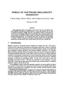
-43. The NVS Error Detection and Recovery Algorithms The original software specifications specified test points, i.e., selected intermediate values of each major system function that had to be provided as outputs for additional error checking. Error detection was easily identified from the test points with some modifications. A further enhancement to the application was the introduction of seven cross-check points (ccp’s)[1] [17], and a recovery point[18]. Error recovery could happen at each cross-check point, and at the recovery point before the result was fed back as input for the next computation. Cross-check points and recovery points were easily specified with their proper format and sequence. The usage of the ccp’s and recovery point in this application program is shown in Figure 2. cc

hhhhhhhhhhhhhc c c c c hhhhhhhhhhhhhhhhh c c Airplane Sensor c c c c Input Generation c chhhhhhhhhhhhhhhhhc c

sensor.input c

hhhhhhhhhhhhhhhhh c Lane Command c c c Computation chhhhhhhhhhhhhhhhhc c c c c c

(lane.input) c c

hhhhhhhhhhhhhhhhh cCommand Monitors,c c c Display Computation chhhhhhhhhhhhhhhhhc c c c c

c hhhhh no Issuing c Recovery? c yes c c state.recovery c hhhhhhhhhhhhhhhhh c c c Recovery c c c Mechanism c chhhhhhhhhhhhhhhhhc c c chhhhhhhhhhhhhc

h hhhhhhhhhhhhhhhhhhhhhhhhhhhhhh c Complementary Filters Processing c c c ccp.filter1, ccp.filter2 c c Mode Logic Processing c c c ccp.modelogic c c Outer Loop Computation c c c ccp.outerloop c c Inner Loop Computation c c ccp.innerloop c hhhhhhhhhhhhhhhhhhhhhhhhhhhhhhc h h hhhhhhhhhhhhhhhhhhhhhhhhhhhhhh c Command Monitors Computation c c ccp.monitors c c c Display Computation c c ccp.display ch hhhhhhhhhhhhhhhhhhhhhhhhhhhhhhc

Figure 2: Usage of Cc-points and Recovery-point in the Application

-5In Figure 2, execution scenario of the application was designed to iterate through the following computations: 1) airplane sensor input generation; 2) lane command computation; 3) command monitors and display computation; and 4) recovery mechanism when necessary. The airplane simulator was separated designed by a coordinating team. Lane command, command monitors and display module were implemented by the programming teams. The recovery mechanism was provided in a supervisory environment[19] [20]. Under this scenario, the application software was instrumented by some fault tolerance mechanisms. Two input points (sensor.input, lane.input) were specified to receive external sensor input from an airplane, and to receive flight commends from the other channels (lanes). Moreover, seven cross-check points (ccp.filter1, ccp.filter2, ccp.modelogic, ccp.outerloop, ccp.innerloop, ccp.monitors, ccp.display) were used to cross-check the results of the major system functions (Complementary Filters, Mode Logic, Outer Loop, Inner Loop, Command Monitors, Display) with the results of the other versions before they were used in any further computation. Finally, One recovery point (state.recovery) was used to recover a failed version by supplying it with a set of new internal state variables that were obtained from the other versions by the Community Error Recovery technique[18]. In summary, these fault tolerance mechanisms introduce 14 external variables (for input functions), 68 intermediate and final variables (for cross-check functions), and 42 state variables (for recovery function) in this application. State variables were identified as those variables whose values in the current iteration would affect their new values in the next iteration. Integrators, filters, and rate-limiters in the system denoted these variables.

4. Software Testing Conducted To emphasize the importance of testing, three phases of testing: unit tests, integration tests, and acceptance tests, were conducted. Different strategies for program testing were provided in order to clean up programs. Table 1 lists the differences among these phases.

-6iiiiiiiiiiiiiiiiiiiiiiiiiiiiiiiiiiiiiiiiiiiiiiiiiiiiiiiiiiiiiiiiiiiii c category c c unit test c integration test c acceptance test c iiiiiiiiiiiiiiiiiiiiiiiiiiiiiiiiiiiiiiiiiiiiiiiiiiiiiiiiiiiiiiiiiiiii iiiiiiiiiiiiiiiiiiiiiiiiiiiiiiiiiiiiiiiiiiiiiiiiiiiiiiiiiiiiiiiiiiii i c cc c c c test criteria ciiiiiiiiiiiiiiiiiiiiiiiiiiiiiiiiiiiiiiiiiiiiiiiiiiiiiiiiiiiiiiiiiiiii c c structure-based c requirements-based c requirements-based c c test case c c open loop by c closed loop by c closed loop by c c cc c c generator PC Basic PC Basic multiple languages cc ciiiiiiiiiiiiiiiiiiiiiiiiiiiiiiiiiiiiiiiiiiiiiiiiiiiiiiiiiiiiiiiiiiiii cc c c c test data c c file i/o by each c interfacing C c interfacing C c c access c c version c routines c routines c iiiiiiiiiiiiiiiiiiiiiiiiiiiiiiiiiiiiiiiiiiiiiiiiiiiiiiiiiiiiiiiiiiiii c cc c c c tested by ciiiiiiiiiiiiiiiiiiiiiiiiiiiiiiiiiiiiiiiiiiiiiiiiiiiiiiiiiiiiiiiiiiiii c c individual teams c individual teams c coordinating team c c tolerance c c 0.01 for degrees c 0.01 for degrees c 0.005 for degrees c c cc c c c level (0.05 for Prolog) ciiiiiiiiiiiiiiiiiiiiiiiiiiiiiiiiiiiiiiiiiiiiiiiiiiiiiiiiiiiiiiiiiiiii cc c c c ciiiiiiiiiiiiiiiiiiiiiiiiiiiiiiiiiiiiiiiiiiiiiiiiiiiiiiiiiiiiiiiiiiiii # of test cases c c 133 c 4 c 9 c c cc c c c total executions c c 1330 ciiiiiiiiiiiiiiiiiiiiiiiiiiiiiiiiiiiiiiiiiiiiiiiiiiiiiiiiiiiiiiiiiiiii c 960 c 18,440 c

Table 1: Different Schemes Used in the Testing Phases The unit test was considered as structure-based test since its test data was provided in such a way to facilitate programmers in hand-tracing the execution of their program units. The integration test and acceptance test, on the other hand, utilized purely requirements-based test data. A reference model of the control laws was implemented and provided by Honeywell Inc. This version was implemented in Basic on an IBM PC to serve as the test case generator for unit tests and integration tests. Criteria of "open loop testing" and "closed loop testing" were used, respectively. Due to the wide numerical discrepancies between this version and the other six program versions under development, a larger tolerance level was chosen. Later in the acceptance test, this reference model proved to be less reliable (several faults were found) and less efficient. Thus, it was necessary to replace it with a more reliable and efficient testing procedure for a large volume of test data. For this procedure, the outputs of the six versions were voted and the majority results were used as the reference points to generate test data during the acceptance tests. This was also the test phase during which programmers were required to submit their programs to the coordinating team and wait for the test results. A finer tolerance level was used based on the observation that less discrepancies were expected if programs computed the right results. An exception had to be made for the Prolog program due to

-7the lack of accuracy in its internal representation of real numbers. In the unit test phase, each module of the program received a variant number of test cases. A total of 133 test cases were executed, and since each test case contained 10 program executions, there were 1330 executions in this phase. Four testing profiles were provided for the integration test. Each test profile contained 12 seconds of flight simulation, a total of 960 executions. These four test data sets differed from each other in the flying modes that were involved (either Altitude Hold Mode only, or from Altitude Hold Mode to Glide Slope Capture and Track Modes), and by the level of wind turbulence (either no wind turbulence or an average wind turbulence) being superimposed. The acceptance test was a stringent testing phase. Nine testing profiles were designed for this test phase. Data sets 1, 3, and 5 executed for 100 seconds, driving the airplane from Altitude Mode to Glide Slope Capture and Track Modes with different magnitude of wind turbulences. Data sets 2, 4, and 6 were designed similarly, except they exercised all five flying modes for 180 seconds. Data sets 7 and 8 were designed to carry out the recovery command, and Data set 9 the Display module. The total executions required in this phase were 18440 program iterations.

5. Software Metrics and Fault Distributions of the Programs Table 2 gives several comparisons of the six versions with respect to some common software metrics. The objective of software metrics is to evaluate the quality of the product in a quality assurance environment. However, our focus here is the comparison among the program versions, since design diversity is our major concern. The following metrics are considered in Table 2: (1) the number of lines of code, including comments and blank lines (LINES); (2) the number of lines excluding comments and blank lines (LN-CM); (3) the number of executable statements, such as assignment, control, I/O, or arithmetic statements (STMTS); (4) the number of programming modules (subroutines, functions, procedures, etc.) used (MODS); (5) the mean number of statements per module (STM/M); (6) the mean number of statements in between cross-check points (STM/CCP); (7) the number of calls to

-8programming modules (CALLS); (8) the number of global variables (GBVAR); (9) the number of local variables (LCVAR); and (10) the number of binary decisions (BINDE). iiiiiiiiiiiiiiiiiiiiiiiiiiiiiiiiiiiiiiiiiiiiiiiiiiiiiiiiiiiiiiiiiiiiiii c Metrics c c ADA c C c MOD-2 c PASCAL c PROLOG c T c c Range c iiiiiiiiiiiiiiiiiiiiiiiiiiiiiiiiiiiiiiiiiiiiiiiiiiiiiiiiiiiiiiiiiiiiiii ciiiiiiiiiiiiiiiiiiiiiiiiiiiiiiiiiiiiiiiiiiiiiiiiiiiiiiiiiiiiiiiiiiiiiii cc c c c c c cc c ciiiiiiiiiiiiiiiiiiiiiiiiiiiiiiiiiiiiiiiiiiiiiiiiiiiiiiiiiiiiiiiiiiiiiii c c 2253 c 1378 c c c 1575 c c 1.64:1 c LINES 1521 c 2234 1733 c cc c c c c c cc c LN-CM 861 c 953 c 1288 1374 ciiiiiiiiiiiiiiiiiiiiiiiiiiiiiiiiiiiiiiiiiiiiiiiiiiiiiiiiiiiiiiiiiiiiiii c c 1517 c c c 1263 c c 1.76:1 c c STMTS c c 1031 c c c 1089 c c 2.56:1 c 746 c 546 c 491 1257 iiiiiiiiiiiiiiiiiiiiiiiiiiiiiiiiiiiiiiiiiiiiiiiiiiiiiiiiiiiiiiiiiiiiiii c cc c c c c c cc c MODS 36 c 26 c 37 c 48 77 44 c c 2.96:1 c ciiiiiiiiiiiiiiiiiiiiiiiiiiiiiiiiiiiiiiiiiiiiiiiiiiiiiiiiiiiiiiiiiiiiiii cc c c c STM/M cc c c 29 c 25 c 15 c 10 16 25 c c 2.90:1 c iiiiiiiiiiiiiiiiiiiiiiiiiiiiiiiiiiiiiiiiiiiiiiiiiiiiiiiiiiiiiiiiiiiiiii c cc c c c c c cc c STM/CCP c c 147 c 107 c 78 c 70 179 156 c c 2.56:1 c ciiiiiiiiiiiiiiiiiiiiiiiiiiiiiiiiiiiiiiiiiiiiiiiiiiiiiiiiiiiiiiiiiiiiiii c c c CALLS cc c c 97 c 68 c 65 c 93 81 87 c c 1.49:1 c iiiiiiiiiiiiiiiiiiiiiiiiiiiiiiiiiiiiiiiiiiiiiiiiiiiiiiiiiiiiiiiiiiiiiii c cc c c c c c cc c GBVAR c c 139 c 141 c 91 c 81 90 97 c c 1.74:1 c ciiiiiiiiiiiiiiiiiiiiiiiiiiiiiiiiiiiiiiiiiiiiiiiiiiiiiiiiiiiiiiiiiiiiiii c c c cc c c LCVAR 117 c 197 c 132 c 127 209 251 c c 2.15:1 c iiiiiiiiiiiiiiiiiiiiiiiiiiiiiiiiiiiiiiiiiiiiiiiiiiiiiiiiiiiiiiiiiiiiiii c cc c c c c c cc c ciiiiiiiiiiiiiiiiiiiiiiiiiiiiiiiiiiiiiiiiiiiiiiiiiiiiiiiiiiiiiiiiiiiiiii cc cc 74 cc 114 cc 78 cc 118 cc 74 cc 86 cc cc 1.59:1 cc c BINDE

Table 2: Software Metrics for the Six Programs A total of 93 faults was found and reported during the whole life cycle of the project. Table 3 shows the test phases during which the faults were detected, and the fault densities (as per thousands of executable statements) of the original version and the accepted version. It also shows test efficiency for fault removal during software development, defined as the number of faults found prior to operational testing divided by the number of total faults. iiiiiiiiiiiiiiiiiiiiiiiiiiiiiiiiiiiiiiiiiiiiiiiiiiiiiiiiiiiiiiiiiiiiiiiiiiiiiiiiii c Test Phase c c ADA c C c MOD-2 c PASCAL c PROLOG c T c c Total c iiiiiiiiiiiiiiiiiiiiiiiiiiiiiiiiiiiiiiiiiiiiiiiiiiiiiiiiiiiiiiiiiiiiiiiiiiiiiiiiii iiiiiiiiiiiiiiiiiiiiiiiiiiiiiiiiiiiiiiiiiiiiiiiiiiiiiiiiiiiiiiiiiiiiiiiiiiiiiiiiii c cc c c c c c cc c Coding/Unit Testing 2 4 4 10 15 7 c c 42 c ciiiiiiiiiiiiiiiiiiiiiiiiiiiiiiiiiiiiiiiiiiiiiiiiiiiiiiiiiiiiiiiiiiiiiiiiiiiiiiiiii cc c c c c c c Integration Testing cc c 5 c c c c 4 c c 20 c 2 0 2 7 iiiiiiiiiiiiiiiiiiiiiiiiiiiiiiiiiiiiiiiiiiiiiiiiiiiiiiiiiiiiiiiiiiiiiiiiiiiiiiiiii c cc c c c c c cc c Acceptance Testing 2 4 0 0 4 ciiiiiiiiiiiiiiiiiiiiiiiiiiiiiiiiiiiiiiiiiiiiiiiiiiiiiiiiiiiiiiiiiiiiiiiiiiiiiiiiii cc c c c c c 10 c c 20 c c cc c c c c c cc Operational Testing 0 5 1 0 3 2 11 c iiiiiiiiiiiiiiiiiiiiiiiiiiiiiiiiiiiiiiiiiiiiiiiiiiiiiiiiiiiiiiiiiiiiiiiiiiiiiiiiii ciiiiiiiiiiiiiiiiiiiiiiiiiiiiiiiiiiiiiiiiiiiiiiiiiiiiiiiiiiiiiiiiiiiiiiiiiiiiiiiiii cc c c c c c cc c ciiiiiiiiiiiiiiiiiiiiiiiiiiiiiiiiiiiiiiiiiiiiiiiiiiiiiiiiiiiiiiiiiiiiiiiiiiiiiiiiii Total c c 6 c 18 c 5 c 12 c 29 c 23 c c 93 iiiiiiiiiiiiiiiiiiiiiiiiiiiiiiiiiiiiiiiiiiiiiiiiiiiiiiiiiiiiiiiiiiiiiiiiiiiiiiiiiic c cc c c c c c cc c Original Fault Density 5.8 c 24.2 c 9.2 c 24.4 23.1 21.1 c c 18.0 c ciiiiiiiiiiiiiiiiiiiiiiiiiiiiiiiiiiiiiiiiiiiiiiiiiiiiiiiiiiiiiiiiiiiiiiiiiiiiiiiiii cc c c ciiiiiiiiiiiiiiiiiiiiiiiiiiiiiiiiiiiiiiiiiiiiiiiiiiiiiiiiiiiiiiiiiiiiiiiiiiiiiiiiii c c 100% c 72% c c 91% c c 88% c Test Efficiency 80% c 100% c 90% c cc c c c c c cc c Operational Fault Density c c 0.0 c 6.7 c 1.8 c 0.0 2.4 2.1 c ciiiiiiiiiiiiiiiiiiiiiiiiiiiiiiiiiiiiiiiiiiiiiiiiiiiiiiiiiiiiiiiiiiiiiiiiiiiiiiiiii c c 1.8 c c

Table 3: Fault Classification by Phases and Other Attributes

-9It is interesting to note that there was only one incidence of an identical fault, committed by two teams, Ada and Modula-2, during program development phase. This fault was due to a comma being misread as a period, which was classified as a specification misinterpretation. During operational testing, two disagreements were traced to an identical fault occurred in the Prolog and T versions, which was due to the programmers’ ignorance to properly incorporate a late specification update. Both pairs of identical faults were related to specification. However, identical faults involving more than two versions have never been observed.

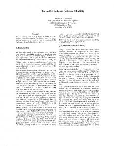
6. N -Version Software System Executions and Results The operational testing of the project was a dynamic, requirements-based testing stressing how the airplane/autopilot interacted and operated in an actual environment. Three channels of diverse software each computed a surface command to guide a simulated aircraft along its flight path. To ensure that significant command errors could be detected, random wind turbulences of different levels were superimposed in order to represent difficult flight conditions. The individual commands were recorded and compared for discrepancies that could indicate the presence of faults. The configuration of the flight simulation system (shown in Figure 3) was consist of three lanes of control law computation, three command monitors, a servo control, an Airplane model, and a turbulence generator.

- 10 hhhhhhhhhhhhhhhhhhhhhhhhhhhhhhhhhhhhhhhhhhhhhhhhhhhhhhhhhhhhhhhhhhhhhhhhhhhhhhhhhhhhhhhhhhhhhhhhhhhhhhhhhhhhhhhhhh c

c

hhhhhhhhhhhhhhhhhhhhhhhhhhhhhhhhhhhhhhhhhhhhhhhhhhhhhhhhhhhhhhhhhhhhhhhh c

hhhhhhhhhhhhhh hhhhhhhhhhhhhh c c c c LANE A c gc c h hhhhhhhhhhhhhhhhhhhhhhhhhhhhhhhhhhhhhhhhhhhhhhh c c g g g c h c cg hhhh c c c COMPUTATION c chhhhhhhhhhhhhhc c c c c c c c c c hhhhhhhhhhhhhh c c c c c COMMAND c c c c c c c hhhhhhhhhhhhhhhhhhhhhhhhhhhhhhhhh c c c c c c c c MONITOR A c c chhhhhhhhhhhhhh c c c c c c c c c c c c c c c c c c c c c c c c c c c c c c c c c c c c c c c c c c c c hhhhhhhhhhhhhh c c c c c c SERVOc c c LANE B c c hhhhhhhhhhhhhhhhhhhhhhh c c c gc h hhhhhhhhhhhhhhhhhhhhhhhhhhhhhhhhhhhhhhhhhhhhhhh c c c g g g c c c c c c cc gh c COMPUTATION c c hhhh c c chhhhhhhhhhhhhhc c c c AIRPLANE / SENSORS / c c c c c c c c hhhhhhhc c c c c CONTROL / h hhhhhhhhhhhhhh c c c c c c c COMMAND c c LANDING GEOMETRY c c c c c c c c c hhhhhhhhhhhhhhhhhhhhhhc c h chhhhhhhhhhhhhhhhhhc c c c c c c MONITOR B c c c chhhhhhhhhhhhhh SERVOS c c c c c c c c c c c c c c c c c c c c c c c c hhhhhhhhhhhhhh c c c c c c c c c c TURBULENCE c c c c c c c c c c c c c GENERATOR c c c c c c chhhhhhhhhhhhhh hhhhhhhhhhhhhh c c c c c c c c LANE C c c c c c c h g g g chhhhhc c hhhhhhhhhhhhhhhhhhhhhhhhhhhhhhhhhhhhhhhhhhhhhhh c c c c c COMPUTATION chhhhhhhhhhhhhhc c c c c c c c c c hhhhhhhhhhhhhh c c COMMAND c c c c c c MONITOR C c cc chhhhhhhhhhhhhh hhhhhhhhhhhhhhc c

c

c c

c c c c c c c c c c c c c c c c c

Figure 3: 3-Channel Flight Simulation Configuration

The lane computations and the command monitors were the redundant software versions generated by the six programming teams. Each lane of independent computation monitored the other two lanes. However, no single lane could make the decision as to whether another lane was faulty. A separate servo control logic function was required to make that decision, based on the monitor states provided by all the lanes. This control logic applied a strategy that ignored the elevator command from a lane when that lane was judged failed by both of the other two lanes, given that these two lanes were judged valid. The aircraft mathematical model provided the dynamic response of current medium size, commercial transports in the approach/landing flight phase. In this model, the airplane was trimmed, by means of flaps and engine thrust setting, to a landing speed of about 120 knots, and a level of low altitude flight path was chosen. It was assumed that the pilot has engaged the autothrottle while in the low-speed, approach condition, so that forward speed variations were

- 11 negligible. In addition, the pilot was assumed to have maneuvered the aircraft to an altitude of 1500 feet in preparation for engagement of the Altitude Hold mode. The three control signals from the autopilot computation lanes were inputs to three elevator servos. The servos were force-summed at their outputs, so that the mid-value of the three inputs became the final elevator command. Sensed airplane attitude, attitude rate, altitude, flight path, and vertical acceleration motions were directly measured by various sensors mounted in the fuselage, which were properly modeled. It was assumed that these sensors were at the center-of-gravity of the aircraft, and had unity gain characteristics. The reaction of the airplane (e.g., the pitch attitude) should be able to stablize the path of the flight in responding to fluctuating inputs. Landing Geometry and Turbulence Generator were models associated with the Airplane simulator. The Landing Geometry mathematical model described the deviation from glideslope beam center as a function of aircraft position relative to the end of the runway. Nominal glideslope beam characteristics were defined by a beam angle of 2.5 degrees referenced to the touchdown point, and a width in the vertical plane of ± 0.5 degrees around the beam center. Interception of the lower edge of the beam by the aircraft resulted in a pitch-over command and acquisition of the beam center. The Turbulence Generator model was used to introduce vertical wind gusts. Vertical turbulence was assumed to be frozen with respect to time. This was based on the observation that for reasonable flight speeds, changes in vertical wind velocity were smaller with respect to time than with respect to position. In summary, one run of flight simulation was characterized by the following five initial values: (1) initial altitude (about 1500 feet); (2) initial distance (about 52800 feet); (3) initial nose up relative to velocity (range from 0 to 10 degrees); (4) initial pitch attitude (range from -15 to 15 degrees); and (5) vertical velocity for the wind turbulence (0 to 10 ft/sec). One simulation consisted of about 5000 iterations of lane command computations (50 milliseconds each) for a total landing time of approximately 250 seconds. In this manner, over 1000 flight simulations (over 5,000,000 program executions) were exercised on the six software versions generated from this

- 12 project. Table 4 shows the errors encountered in each single version, while Table 5 shows different error categories under all combinations of 3-version and 5-version configurations. Note that the discrepancies encountered in the operational testing were called "errors" rather than "failures" due to their non-criticality in the landing procedure, i.e., a proper touchdown was still achieved. iiiiiiiiiiiiiiiiiiiiiiiiiiiiiiiiiiiiiiiiiiiiiiiiiiiiiiiii c c c c number of c c size total error c version c c c c (l.o.c.) executions errors probability c iiiiiiiiiiiiiiiiiiiiiiiiiiiiiiiiiiiiiiiiiiiiiiiiiiiiiiiii iiiiiiiiiiiiiiiiiiiiiiiiiiiiiiiiiiiiiiiiiiiiiiiiiiiiiiii i c c c c c c 2256 0 c Ada c c 5127400 c c .0000000 c 1531 568 c C c c 5127400 c c .0001108 c c Modula-2 c 1562 c 5127400 c 0 c .0000000 c c Pascal c c 5127400 c c .0000000 c 2331 0 c Prolog c c c c .0001326 c 2228 5127400 680 c c c c c T 1568 5127400 c 680 .0001326 cc i iiiiiiiiiiiiiiiiiiiiiiiiiiiiiiiiiiiiiiiiiiiiiiiiiiiiiiii i c iiiiiiiiiiiiiiiiiiiiiiiiiiiiiiiiiiiiiiiiiiiiiiiiiiiiiiii c c c Average c 1913 321 c 5127400 c c .00006267 c ciiiiiiiiiiiiiiiiiiiiiiiiiiiiiiiiiiiiiiiiiiiiiiiiiiiiiiiii

Table 4: Errors in Individual Versions iiiiiiiiiiiiiiiiiiiiiiiiiiiiiiiiiiiiiiiiiiiiiiiiiiiiiiiii c c 3-version configuration c c 5-version configuration c c cate- iiiiiiiiiiiiiiiiiiiiiiiiiiiiiiiiiiiiiiiiiiiiiiiiii c c c c c c c c c c gory c # of cases c probability c c # of cases c probability cc i iiiiiiiiiiiiiiiiiiiiiiiiiiiiiiiiiiiiiiiiiiiiiiiiiiiiiiii i c iiiiiiiiiiiiiiiiiiiiiiiiiiiiiiiiiiiiiiiiiiiiiiiiiiiiiiii c c 1. .9998409 .9997807 c ciiiiiiiiiiiiiiiiiiiiiiiiiiiiiiiiiiiiiiiiiiiiiiiiiiiiiiiii c 102531685 c c c 30757655 c ciiiiiiiiiiiiiiiiiiiiiiiiiiiiiiiiiiiiiiiiiiiiiiiiiiiiiiiii c cc 2. 13385 c .0001305 5890 c .0001915 c c c c c 3. 210 c .000002048 c c 70 c .000002275 cc i c iiiiiiiiiiiiiiiiiiiiiiiiiiiiiiiiiiiiiiiiiiiiiiiiiiiiiiii c 4. 2720 cc .00002652 c c 680 cc .00002210 c ciiiiiiiiiiiiiiiiiiiiiiiiiiiiiiiiiiiiiiiiiiiiiiiiiiiiiiiii c ciiiiiiiiiiiiiiiiiiiiiiiiiiiiiiiiiiiiiiiiiiiiiiiiiiiiiiiii c cc 5. 105 c .000003413 c c iiiiiiiiiiiiiiiiiiiiiiiiiiiiiiiiiiiiiiiiiiiiiiiiiiiiiiiii c c c c c Total c 102548000 cc 1.0000000 ciiiiiiiiiiiiiiiiiiiiiiiiiiiiiiiiiiiiiiiiiiiiiiiiiiiiiiiii c c 30764400 cc 1.0000000 c

classifications of the category: 1 - no errors 2 - single errors in one version 3 - two distince errors in multiple versions 4 - two coincident errors in multiple versions 5 - three errors in multiple versions Table 5: Errors in 3-Version and 5-Version Execution Configurations

From Table 4 we can see that the average error probability for single version is .00006267.

- 13 Table 5 shows that for all the 3-version combinations, the error probability concerning reliability is .00002857 (categories 3 and 4), and that for safety is .00002652 (category 4). This is a reduction of roughly 2.3. In all the combinations of 5-version configuration, the error probability for reliability is .000003413 (category 5; Two of the three errors are coincident, resulting in nodecision), a reduction by a factor of 18. This probability becomes zero in the safety measurement. From these numbers it might be interpreted that the expected dependability improvement of NVS over single-version software is quite moderate. However, it is noted that the coincident errors produced by the Prolog and T programs were all caused by one identical fault in both versions, which was due to the ignorance of a slight specification update that was made very late in the programming process. This fault manifested itself right after these program versions were put together for the flight simulation. Had this fault been eliminated in the operational testing, categories 3, 4 and 5 for both 3-version and 5-version configurations in Table 5 would have been all zero, resulting in perfect dependability figures.

7. Fault Diagnosis and Error Analysis by Mutation Testing To uncover the impact of faults that would have remained in the software version, and to evaluate the effectiveness of NVS mechanisms, a special type of regression testing, similar to mutation testing which is well known in the software testing literature[21] [22], was investigated in the six versions. The original purpose of the mutation testing is to ensure the quality of the test data used to verify a program, while our concern here was to examine the relationship of faults and error frequencies in each program and to evaluate the similarity of program errors among different versions. The testing procedure is described in the following steps: 1) The fault removal history of each program was examined and each program fault was analyzed and recreated. 2) Mutants were generated by injecting faults one by one into the final version from where they were removed (i.e., a fault from the C program will be injected to the C program only). Each mutant contains exactly one known software fault. 3) Each mutant was executed by the same set

- 14 of input data in the Airplane simulation environment to observe errors. 4) Analyze the error characteristics to collect error statistics and correlations. Using the fault removal history of each version, we created 6 mutants for Ada (a1 - a6), 18 mutants for C (c1 - c18), 5 mutants for Modula-2 (m1 - m5), 12 mutants for Pascal (p1 - p12), 29 mutants for Prolog (pg1 - pg29), and 23 mutants for T (t1 - t23). A higher index number in each mutant represents the injection of a later fault to that version. In order to present the execution results of the above procedure, let us define the following two functions for each mutant: g

Error Frequency Function (for a given set of test data) − the frequency of the error being triggered by the specified test data set in this mutant.

g

Error Severity Function (for a given set of test data) − the severity of the error when manifested in the system by the specified test data set.

An Error Frequency Function of version x mutant i for test set τ, denoted as λ(xi ,τ), is computed by total number of errors when executing test set τ on mutant xi λ(xi ,τ) = hhhhhhhhhhhhhhhhhhhhhhhhhhhhhhhhhhhhhhhhhhhhhhhhhhhhhh total number of executions Since each mutant contains only one known fault, it is hypothesized that errors produced by that fault are always the same for the same test inputs[23]. This hypothesis is considered valid for all the mutants discussed here. Therefore, we can define an Error Severity Function of version x mutant i for test set τ, µ(xi ,τ), to be

µ(xi ,τ) =

I J J J0 J K J ref erence value − error of x J i J J hhhhhhhhhhhhhhhhhhhhhhhhhh J ref erence value J JJ J J1 L

J

J

J

J

ref erence value − error of xi J , if 0 < J hhhhhhhhhhhhhhhhhhhhhhhhhh