Solving Goal Programming Problems Using Multi-Objective Genetic Algorithms Kalyanmoy Deb Kanpur Genetic Algorithms laboratory (KanGAL) Department of Mechanical Engineering Indian Institute of Technology, Kanpur Kanpur, PIN 208 016, India
[email protected]
Abstract- Goal programming is a technique often used in engi-
Steuer, 1986), these methods are also not free from the dependence on the relative weight factor for each criterion function. In this paper, we suggest using a multi-objective genetic algorithm (CA) to solve the goal programming problem. In order to use a multi-objective GA, each goal is converted into an equivalent objective function. Unlike the weighted goal programming method, the proposed approach does not add any artificial constraint into its formulation. Since, multiobjective GAS have been shown to find multiple Paretooptimal solutions (Fonseca and Fleming, 1993; Srinivas and Deb, 1995), the proposed approach is likely to find multiple solutions to the goal programming problem, each corresponding to a different setting of the weight factors. This makes the proposed approach independent from the user. Moreover, since no explicit weight factor for each criterion is used, the method is also not likely to have any difficulty in finding solutions for problems having non-convex feasible, decision space. It is worthwhile to highlight here that the use of a multiobjective optimization technique to solve goal programming problems is not new (Romero, 1991, Steuer, 1986). But the inefficiency of classical non-linear multi-objective optimization methods has led the researchers and practitioners to concentrate on solving linear goal programming problems only. Although there exist some attempts to solve linear approximations of a non-linear problem sequentially, these methods have not been efficient (Romero, 1991). Multi-objective GAS are around for last five years and have been shown to solve various non-linear multi-objective optimization problems successfully (Eheart, Cieniawski, and Ranjithan, 1993; Parks and Miller, 1998; Weile, Michelsson, and Goldberg, 1996). As a result of these interests, there exist now a number of multi-objective CA implementations (Fonseca and Fleming, 1993; Horn, Nafploitis, and Goldberg, 1994; Srinivas and Deb, 1995; Zitzler and Theile, 1998). In this paper, we show for the first time how one such GA implementation can make non-linear goal programming easier and practical to use.
neering design activities primarily to find a compromised solution which will simultaneously satisfy a number of design goals. In solving goal programming problems, classical methods reduce the multiple goal-attainment problem into a single objective of minimizing a weighted sum of deviations from goals. In this paper, we pose the goal programming problem as a multiobjective optimization problem of minimizing deviations from individual goals. This procedure eliminates the need of having extra constraints needed with classical formulations and also eliminates the need of any user-defined weight factor for each goal. The proposed technique can also solve goal programming problems having non-convex trade-off region, which are difficult to solve using classical methods. The efficacy of the proposed method is demonstrated by solving a number of test problems and by solving an engineering design problem. The results suggest that the proposed approach is a unique, effective, and practical tool for solving goal programming problems.
1 Introduction Developed in the year 1955, goal programming method has enjoyed innumerable applications in engineering design activities (Charnes, et al., 1955; Clayton et al., 1982; Ignizio, 1976, 1978). Goal programming is different in concept from non-linear programming or optimization techniques in that the goal programming attempts to find one or more solutions which satisfy a number of goals to the extent possible. Instead of finding solutions which absolutely minimize or maximize objective functions, the task is to find solutions that, if possible, satisfy a set of goals, otherwise, violates the goals minimally. This makes the approach more appealing to practical designers compared to optimization methods. The most common approach to classical goal programming techniques is to construct a non-linear programming problem (NLP) where a weighted sum of deviations from targets is minimized (Romero, 1991). The NLP problem also contains a constraint for each goal, restricting the corresponding criterion function value to be within the specified target values. A major drawback with this approach is that it requires the user to specify a set of weight factors, signifying the relative importance of each criterion. This makes the approach subjective to the user. Moreover, the weighted goal programming approach has difficulty in finding solutions in problems having non-convex feasible decision space. Although there exists other methods such as lexicographic goal programming or minimax goal programming (Romero, 1991, 0-7803-5536-9/99/$10.00 01999 IEEE
2 Goal Programming Goal programming was first introduced in an application of a single-objective linear programming problem by Charnes, Cooper, and Ferguson (1955). However, goal programming gained popularity after the works of Ignizio (1976), Lee (1972), and others. Romero (1991) presented a comprehensive overview and listed a plethora of engineering applications where goal programming technique has been used. The 77
+
function, so that f(2) n 2 t. The deviation n quantifies the amount by which the critexion function has not satisfied the target t. Here, the objective of goal programming is to minimize the deviation n. For f(i) < t, the deviation n should take a nonzero positive value, otherwise it must be zero. For the equal-to type goal, both deviations are used, so that f(l) - p n = t. Here, the objective of goal programming is to minimize a weightad sum (crp ,&), so that the obtained solution is minimally away from the target in either direction. The fourth type of goal is handled by using two constraints: f(i) - p 5 t‘ and f(i) n 2 tu. The objective here is to minimize the summation ( a p ,On).All of the above constraints can be replaced by a generic equality constraint: f(i)- p + n = t . (2)
main idea in goal programming is to find solutions which attain a pre-defined target for one or more criterion function. If there exists no solution which achieves targets in all criterion functions, the task is to find solutions which minimize deviations from targets. Goal programming is different from non-hear programming (constrained optimization) problems (NLPs), where the main idea is to find solutions which optimizes one or more criteria (Deb, 1995; Reklaitis et al., 1983). Let us consider a design criterion f(i), which is a function of a solution vector 5. In the context of NLP, the objective is to find the solution vector Z* which will minimize or maximize f(Z). Without loss of generality, we assume that the criterion function f(Z) is to be minimized. In most design problems, there exists a number of constraints which make a certain portion (Z E F)of the search space feasible. It is imperative that the optima! solution Z* is feasible, that is, i’ E F. In a goal programming, a target value t is chosen for every design criterion. One of the design goals may be to find a solution which attains a cost o f t : goal (f(Z) = t ) , Subject to i E F.
+
+
+
+
For a ‘less-than-equal-to’type goal, the deviation n is a slack variable which makes the inequality constraint into an equality constraint (Deb, 1995). For a ‘range’ type goal, there are two such constraints, one with t‘ having p as the slack variable and the other with t u having n as the slack variable. Thus, a goal programming problem is converted into an NLP problem where each goal is converted to at least one equality constraint and the objective is to minimize all deviations p and n. Goal programming methods differ in the way the deviations are minimized. Here, we briefly discuss three popular methods.
(1)
If the target cost t is smaller than the minimum possible cost f ( P ) ,naturally there exists no feasible solution which will attain the above goal exactly. The objective of goal programming is then to find that solution which will minimize the deviation d between the achievement of goal and the aspiration target, t. The solution for this problem is i* and the overestimate is d = f(Z*) - t. Similarly, if target cost t is larger than the maximum feasible cost fmax, the solution to the goal programming problem is 5 which makes f(Z) = fmax. HowfmaX], the solution ever, if the target cost !I is within [f(Z*), to the goal programming problem is that feasible solution i which makes the criterion value exactly equal to t. In the above example, we have considered a singlecriterion problem. Goal programming brings interesting scenarios when multiple criteria are used. In the above example, an ‘equal-to’ type god is discussed. However, there can be four different types of goal criteria:
2.1 Weighted Goal Programming A composite objective function with deviations from each of M criterion function is used: Minimize Subject to
(crjpj
-I+p j n j ) ,
- p j + ozj = t j , for each goal j,
f j (5)
ZE 3 nj,Pj
2 0,
for each goal j.
(3) Here, the parameters a j and P j are weighting factors for positive and negative deviations of the j-th criterion function. For less-than-equal-to type goals, the parameter /3j is zero. Similarly, for greater-than-equal-to type goals, the parameter aj is zero. For range-type goals, there exists a pair of constraints for each criterion function. Usually, the weight factors aj and P j are fixed by the user, a matter which makes the method subjective to the user. We illbstrate this matter through an example problem:
1. Less-than-equal-to (f(2) 5 t),
2. Greater-than-equal-to (f(Z)2 t ) , 3. Equal-to ( f ( i ) = t ) ,and 4. Within a range (f(Z) E [t’,t”]). In order to tackle each of the above goals, usually two nonnegative deviation variables (p and n) are introduced. For the less-than-equal-to type goal (f(Z) t), the positive deviation p is subtracted from the criterion function, so that f (2) - p 5 t . Here, the deviation p quantifies the amount by which the criterion value has surpassed the target t (Ignizio, 1978). If f(Z) > t, the deviation p should take a non-zero positive value, otherwise it must be zero. Here the objective of goal programming is to minimize p . For the greaterthan-equal-to type goal, a deviation n is added to the criterion
goal
l), a solution x ( I ) is said to dominate the other solution d 2 )if , both the following conditions are true (Steuer, 1986):
be able to respond to differing weight factors in problems having non-convex feasible decision space. For handling other types of goals, an Archimedian contour with an equivalent penalty function is used (Steuer, 1986). Figure 3(b) shows the penalty function used for an ‘equal-to’ type goal, involving two weights cr and p.
2.2 Lexicographic Goal Programming In this approach, different goals are categorized into several levels of preemptive priorities. Goals with a lower-level priority is infinitely more important than a goal of a higher-level priority. Thus, it is important to fulfill the goals of first level priority before considering goals of second level of priority. This approach formulates and solves a number of sequential goal programming problems. First, only goals and corresponding constraints of the first level priority are considered. If there exists multiple solutions to the problem, another goal programming problem is formulated with goals having the second level priority. In this case, the objective is only to minimize deviation in goals of the second level priority. However, the goals of first level priority is used as hard constraints. This process continues with goals of other higher level priorities in sequence. The process is terminated as soon as one of the goal programming problems results in a single solution. Since solving an individual goal programming requires the use of the weighted goal programming approach for nonlinear problems, this method is also not free from the subjectiveness of users and other difficulties mentioned earlier.
< denotes worse and + denotes better) than d 2 )in all objectives, or f j ( ~ ( ~ 1A ) f j (d’)) for all j = 1 , 2 , . . . , M objectives.
1. The solution dl) is no worse (say the operator
2. The solution dl) is strictly better than d 2 )in at least one o objective, or fj(d’))+ f j ( d 2 ) ) for at least one 3 E {1,2,. . . , M } . With these conditions, it is clear that in a population of N solutions, the set of non-dominated solutions are likely candidates to be the members of the Pareto-optimal set. In the following, we describe one multi-objective GA which attempts to find the best set of non-dominated solutions in the search space.
3.1 Non-dominatedSorting GA (NSGA) NSGA varies from a simple genetic algorithm (Goldberg, 1989) only in the way the seilection operator in used. The crossover and mutation operators remain as usual. Before the selection is performed, the population is first ranked on the basis of an individual’s non-domination level and then a dummy fitness is assigned to each population member.
2.3 Minimax Goal Programming This approach is similar to the weighted goal programming approach, but instead of minimizing the weighted sum of deviations from targets, the maximum deviation in any goal from target is minimized. Once again, this method requires the choice of weight factors, thereby making the approach subjective to user. In the next section, we briefly discuss multi-objective GAS. Thereafter, we show how multi-objective GAS can be used to solve goal programming problems which do not need any weight factor. In fact, the proposed approach simultaneously finds solutions to the same goal programming problem formed for different weight factors, thereby making the approach both practical and different from the classical approaches.
3.1.1 Fitness Assignment Consider a set of N population members, each having M (> 1) objective function values. Each solution is compared with all other solutions in the population for domination according to the above two conditions. All non-dominated solutions are assumed to constitute the first non-dominated front in the population and are assigned a large dummy fitness value (we assign a fitness N), The same fitness value is assigned to give an equal reproductive potential to all these nondominated individuals. In order to maintain diversity in the population, these non-dominated solutions are then shared (a procedure discussed later) with their dummy fitness values. Sharing is achieved by dividing the dummy fitness value of an individual by a quantity (called the niche count) proportional to the number of individuals around it. This procedure causes multiple optimal solutions to co-exist in the population. The worst shared fitness value in the solutions of the first non-dominated front is noted for further use.
3 Multi-ObjectiveGenetic Algorithms Multi-objective optimization problems give rise to set of Pareto-optimal solutions, none of which can be said to be better than other in all objectives (Steuer, 1986). Thus, it is also a goal in a multi-objective optimization to find as many such Pareto-optimal solutions as possible. Unlike most classical
80
After sharing, these non-dominated solutions are ignored temporarily and new set of non-dominated solutions are found using the above two conditions for domination. A dummy fitness value which is a little smaller than the worst shared fitness value observed in solutions of the first nondominated set is assigned to each of these second-level nondominated solutions. Thereafter, the sharing procedure is performed among them and shared fitness values are found as before. This process is continued till all population members are assigned a shared fitness value. The population is then reproduced with their shared fitness values. A stochastic remainder proportionate selection (Goldberg, 1989) is used in this study. Since individuals in the first front have a better fitness value than solutions of any other front, they always get more copies than the rest of population. This was intended to search for non-dominated regions, which will finally lead to the Pareto-optimal front.
3.1.2 Sharing Procedure Given a set of n k solutions in the k-th non-dominated front each having a dummy fitness value fk, the sharing procedure works by computing a normalized Euclidean distance measure between i-th and j-th solutions:
where P is the number of variables in the problem. The parameters x; and x; are the upper and lower bounds of variable xp. Thereafter, a sharing function value is calculated using
Sh(Sij) =
{A
-
(&)'
i
if6ij
5 ushare,
otherwise.
1
For the i-th solution, a niche count is computed by adding sharing function value with all other solutions: m, = Sh(bij). Finally, a shared fitness valwis computed by degrading the dummy fitness of i-th solution: f;' = fk/mi. This procedure is continued for all i = 1 , 2 , . . . , nk and a corresponding f,!is found. Thereafter, the smallest value fFlnof all f: in the k-th non-dominated front is found for further processing. The dummy fitness of the next non-dominated front is assigned to be fk+l = - E k , where 6k is a small positive number. The above sharing procedure requires a prespecified parameter Ushare, which can be calculated as follows (Deb and Goldberg, 1989):
cy:,
frin
4 Proposed Technique The goal programming problem can be modified suitably to solve using multi-objective GAS. Each goal is converted to an objective of minimizing the deviation from target: Objective function Minimize (f3(2) - t,) goal Cf, ( 5 )I t 3 ) Minimize ( t , - f,( 2 ) ) goal (f,(q 2 t 3 ) Minimize If, ( 2 )- t, I goal (f,( 2 ) = t, 1 Range goal (f,(Z) E [ti,t;]) Min. max((t: - f3(2)), Here the bracket operator ( ) returns the value of the operand if the operand is positive, otherwise returns zero. Although other methods have been suggested in classical goal programming texts (Romero, 1991; Steuer, 1986), the advantage with the above formulation is that (i) there is no need of any additional constraint for each goal, (ii) since GAS do not require objective functions to be differentiable, the above objective function can be used, and (iii) multiple solutions corresponding to a different set of weight factors can be obtained simultaneously. The proposed method allows one to find multiple solutions corresponding to different weight factors simultaneously. After multiple solutions are found, designers can then use higher-level decision-making approaches or compromise programming (Zeleney. 1973) to choose one particular solution. Each solution can be analyzed to find the relative importance of each criterion function as follows: (7)
For a 'range' type goal, the target t j can be substituted by either tf or tY depending on which is closer to f (Z). Moreover, the proposed approach also does not pose any other difficulties that the weighted goal programming method has. Since solutions are compared criterion-wise, there is no danger of comparing butter with potatoes, nor there is any difficulty of scaling in criterion function values. Furthermore, we shall show in the next section that this approach allows to find critical solutions to certain type of goal programming problems which the weighted goal programming method cannot find.
5 Proof-of-PrincipleResults We apply the proposed technique to solve a number of goal programming problems. 5.1 Test Problem PI We first consider the example problem given in equation 4. The goal programming problem is converted into a twoobjective optimization problem as follows:
where q is the desired number of distinct Pareto-optimal solutions. It has been been shown elsewhere (Srinivas and Deb, 1995) that the use of above equation with q M 10 works in many test problems.
Minimize ( f l ( z l r x z ) - 2), Minimize (fz(x1, x2) - a), Subject to F (0.1 5 21 5 1, 0 5 xz
=
81
(8)
5 10).
Here, the criterion functions are fi = 10x1 and f2 = (10 (z2 - 5)2)/(10z1). We use a population of size 50 and run NSGA for 50 generations. A Ushare = 0.158 (equation 6 with P = 2 and q = 10) is used. Each variable is coded in a 20-bit string. As discussed earlier, the feasible decision space lies above the hyperbola. All 50 solutions in the initial population and all non-dominated solutions at the final population are shown in Figure 4, which is plotted with criterion function values f1 and f2. All final solutions have
Here, the first goal is of 'greater-than-equal-to' type and the second goal is of 'equal-to' type. The feasible decision space is the region above the circle shown in Figure 5. The criterion space is the line AB. Since there is no feasible solution which lies in the criterion space, the solution to this goal programming problem is the region on the circle marked by the dashed lines. Each solution in this region corresponds to a goal programming problem with a specific set of weight factors. The solutions to this problem are g2 = 0 and 0.71794 5 gl 5 0.9, depending on the weight factors used. To solve using NSGA, the above problem is converted into an equivalent two-objective optimization problem, as follows:
+
'
I
I
I
I
Minimize (0.9 - f 1 ( 2 1 , 2 2 ) ) , Minimize 1f2(t1, c,) - 0.551, Subjectto 0 5 t l 5 1, 0 5 t
(10) 2
5 1.
Same NSGA parameters as that in test problem P1 are used here. Figure 5 shows how NSGA has able to find many solutions in the desired range in a single run. All 50 initial pop2
0
6
4 f-
8
t!2%?58
10
1
= 5.0 and 0.2 5 cl 5 0.5. The figure also marks the region (with dashed lines) of true solutions of this goal programming problem with different weight factors. The figure shows that NSGA in a single run has been able to find different solutions in the desired range. Table 1 shows five different solutions obtained by the NSGA. Relative weight factors for each solution are also computed using equation 7. If the first criterion is of more importance, solutions in first and second row can be chosen, whereas if second criterion is of more importance solutions in fourth or fifth rows can be chosen. The solution in the third row shows a solution where both criteria are of more or less equal importance. The advantage of us-
E,
-
0.6 0.5 0.4
0.3
Cl
&
5.0228
I flm
h(Z)
2.0289
4.9290
I
I
I
w1
w2
0.9902
0.0098
0
1
'
O
0.2
0.4
cI
0.6
0.8
5.3 Test Problem P3 Next, we consider a goal programming problem which will cause the weighted goal p r o g r m i n g approach difficulty in finding most of the desired solutions. This problem is a simple modification to problem Pa: goal (f1 = c1 E [0.25,0,75]), 102;) goal (f2 = (1 Subjectto 0 5 11 5 1, 0 5 22 5 1.
ing the proposed technique is that all such (and many more as shown in Figure 4) solutions can be found simultaneously in one single run.
(11)
We use the following goal programming problem:
+ 102;) = 0.55), 05
22
5 1.25),
Figure 6 shows the decision space and the criterion space in a f l - f 2 plot. Once again, there is no feasible solution which satisfies both goals. The solutions to the above problem lie on the circle in the region AB and CD, since each solution in the region will make the deviations from the criterion space minimum for a particular set of weight factors. With the weighted goal programming method, it is expected to find the solutions A, B, C, or D only. One Archimedian contour line with the shortest weighted deviation is shown by the dashed line. When a different combination of weight factors is chosen, no
5.2 Test Problem P2
d-)(l
I
ulation members could not ba shown in the figure, because many solutions lie outside the plotting area.
+d m ) ( l +
goal (f1 = 11 2 0.9), goal (f2 = (1Subject to 0 5 11 5 1,
I
Figure 5: NSGA solutions are shown on a f i -f2 plot of problem P2.
Table I: Five solutions to the eo81 . Droeramming -.Droblern are shown. 0.2029
Dcrision Space
0.8
Figu,re4: NSGA solutions are shown on a f~-f2 plot of problem P1.
5 1. (9)
82
I .6 1.J
15
1.4
1.4
7
1.3
1.3
I '
1.2
1.2
1.1
I.,
I , 0
0.2
06
0.4
0.8
. . :
I
I
I
I
0
0.4
0.2
tI
0.6
I
0.8
1-1
Figure 6: Criterion and decision spaces are shown for test problem
Figure 7: NSGA solutions are shown on a fl-fi plot of test problem P3.
P3.
such contour can become tangent to any other point within AB or CD. Thus, the intermediate solutions cannot be found using the weighted goal programming approach. However, if a two-sloped penalty function (as shown in Figure 3(c)) is used, such intermediate solutions (with contour shown by the dotted lines) can be found. This two-slope method requires user to choose two weight factors ( a and a') for each goal. Moreover, the difficulty of dependence of the resulting solution on the weight factors still remains. We use NSGAs with a population size of 100 and with all other parameters same as that used earlier. The solutions after 50 generations are shown in Figure 7. The figure shows that solutions in both regions AB and CD are found by the NSGA in one single run.
If there exists a solution which satisfies both goals, that would be the desired solution. But, if such a solution does not exist, we are interested in finding a solution which will minimize the deviation in cost and deflection from 5 and 0.001, respectively. The need of such penalty parameters can be avoided by using an efficient constraint handling approach (Deb, in press). There are four constraints, restricting shear, normal, and buckling considerations (Reklaitis et al., 1983). A violation of any of these constraints will make the design unacceptable. Thus, in terms of discussion in Ignizio (1986), satisfaction of these constraints is the first priority. We handle these constraints using the bracket-operator penalty function (Deb, 1995). Penalty parameters of 100 and 0.1 are used for the first and second criterion functions, respectively. In order to investigate the search space, we plot many random feasible solutions in f 1 - f ~ space in Figure 9. The
6 An Engineering Design A beam needs to be welded to another beam and must carry a certain load F (Figure 8). It is desired to find four design
0
Figure 8: The welded beam design problem.
5
10
15
20
25
30
35
40
COS1
Figure 9: NSGA solutions (each marked with a 'diamond') are shown on objective function space.
parameters (thickness of the beam, b, width of the beam t , length of weld t, and weld thickness h) for which the fabrication cost of the beam is at most 5 units and end-deflection of the beam is at most 0.001 inch:
corresponding criterion space (cost 5 5 and deflection 5 0.001) is also shown in the figure. The figure shows that there exists no feasible solution in the criterion space, meangoal (fi(.') = 1.10471h2t 0.04811tb(14.0+ t) 5 5), ing thereby that the solution to the above goal programming goal (fZ(Z) = 5 0.001), problem will have to violate at least one goal. The realparameter NSGA with 100 population members, the SBX Subject to SI(.') E 13,600 - T(.') 2 0, operator with qc = 30 and the polynomial mutation operag2(.') 3 30,000 - U ( . ' ) 2 0, tor with qm = 100 are used. w e also use dshare of 0.281 g3(Z) E b - h 2 0, (refer to equation 6 with P = 4 and q = 10). Figure 9 shows g4(Z) Pc(.') - 6,000 2 0. 0 . 1 2 5 ~ h , b < 5 . 0 , a n d O . l ~ ~ , t < l O . O . the solutions (each marked with a 'diamond') obtained after 500 generations. Each solution can be accounted for a dif(12)
*
+
83
Deb, K. and Agrawal, R. B. (1995) Simulated binary crossover for continuous search space. Complex Systems, 9 115-148. Deb, K. and Goldberg, D. E. (1989). An investigation of niche and species formation in genetic function optimization. Pro-
ferent combination of weight factors of cost and deflection quantities (Table 2). If cost is more important than deflec-
Cost Defl. 5.70 0.0033 10.02 0.0018 16.76 0.0010
ceedings of the Third International Conference on Genetic Algorithms (pp. 42-50).
e
t b w l w z 0.627 1.644 9.996 0.662 0.94 0.06 0.778 1.274 9.999 1.247 0.43 0.57 1.032 0.890 9.998 2.194 0.00 1.00 h
Eheart, J. W., Cieniawski, S . E., andRanjithan,S.(1993). Geneticalgorithm-based design cif groundwater quality monitoring system. WRC Research Report No. 218. Urbana: Department of Civil Engineering, The University of Illinois at Urbana-Champaign.
tion, the weight factor (computed using equation 7) for cost will be more and a solution like the first solution will be chosen. On the other hand, if deflection is important, a solution like the third solution will be chosen. Depending on the relative weights of cost and deflection, other solutions such as the second solution in the table will be chosen.
Fonseca, C. M. and Fleming, P.J. (1993). Genetic algorithms for multi-objective optimizadon: Formulation, discussion and generalization. Proceedings of the Fifth International Conference on Genetic Algorithms. 416-423. Goldberg, D. E. (1989). Genetic algorithms for search, optimization, and machine learning. Reading, MA: Addison-Wesley. Horn, J. and Nafploitis, N., and Goldberg, D. E. (1994). A niched Pareto genetic algorithm for multi-objective optimization.
7 Conclusions Classical methods used for solving goal programming problems require users to provide a weight factor for each goal. The resulting solution, therefore, depends on the chosen set of weight factors. Moreover, the popular weighted goal programming problem has the difficulty of finding important solutions in problems having non-convex feasible decision space. In this paper, we reformulate the goal programming problem into a multi-objective optimization problem and suggest using a multi-objective GA to find desired solutions. Since multi-objective GAS can find multiple Pareto-optimal solutions in one single run, the proposed technique is capable of finding multiple solutions to the goal programming problem, each corresponding to a different set of weight factors. The efficacy of the proposed technique has been shown by solving three test problems and one engineering design problem. The results are encouraging and suggest the use of the proposed approach to more complex and real-world engineering goal-programming problems.
Proceedings of the First lEEE Conference on Evolutionary Computation. 82-87.
Ignizio, J. P. (1976). Goal programming and extensions. Lexington, MA: Lexington Books. Ignizio, J. P. (1978). A review of goal programming: A tool for multiobjective analysis. Journal of Operations Research Society, 29(11), 1109-1119, Lee, S. M. (1972). Goal programming for decision analysis. Philadelphia: Auerbach pbblishers. Parks, G. T. and Miller, I. (1998). Selective breeding in a multiobjective genetic algorithm. Proceedings of the Parallel Problem Solvingfrom Narure, V, 250-259. Reklaitis, G. V., Ravindran, A. and Ragsdell, K. M. (1983). Engineering optimization methods and applications. New York: Wiley. Romero, C. (199I). Handbook of critical issues in goal programming. Oxford: Pergamon Press. Srinivas, N. and Deb, K. (1995). Multi-Objective function optimization using non-dominated sorting genetic algorithms, Evolutionary Computation, 2(3), 22 1-248. Steuer, R. E. (1986). Multiple criteria optimization: Theory, computation, and application. New York: Wiley. Weile, D. S., Michielssen, E., and Goldberg, D. E. (1996). Genetic algorithm design of Pareto-optimal broad band microwave absorbers. IEEE Transactions on Electromagnetic Compatibility, 38(4). Zitzler, E. and Thiele, L. (1998a). Multiobjective optimization using evolutionary algorithms-A comparative case study. Parallel Problem Solving from Nature, V , 292-301. Zeleney, M. (1982).Multiple clriteria decision making. New York: McGraw-Hill. Zeleney, M. (1973). Compromise programming. In J. L. Cochrane and M. Zeleney (Eds.) Multiple criteria decision making, (pp. 262-301).
Acknowledgments The author acknowledges the support from Alexander von Humboldt Foundation, Germany.
References Charnes, A., Cooper, W., and Ferguson, R. (1955). Optimal estimation of executive compensation by linear programming. Management Science, I, 138-1 5 1. Clayton, E. R., Weber, W. E., and Taylor, B. W. (1982). A goal programming approach to the optimization of multiresponse simulation models. IIE Transactions, 14(4), 282-287. em Deb, K. (in press). An efficient constraint handling method for genetic algorithms. Computer Methods in Applied Mechanics and Engineering.
Deb, K. (1995). Optimization for engineering design: Algorithms and examples. New Delhi: Prentice-Hall.
84