Linear Programming is a strong tool for many real-life optimization problems. We
can solve large problems (thousands of constraints and millions of variables).
Motivation
Vehicle Routing
Scheduling
Production Planning
Solving Real-Life Problems with Integer Programming Jesper Larsen1 1 Department
of Management Engineering Technical University of Denmark
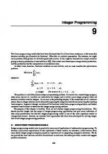
42113 Network and Integer Programming
Motivation
Vehicle Routing
Scheduling
Production Planning
Linear Programming Linear Programming is a strong tool for many real-life optimization problems. We can solve large problems (thousands of constraints and millions of variables). We can solve problems fast (even big problems with hundreds of constraints and thousands of variables solve in seconds or fractions hereof). We can model a lot of problem type and using a modelling language (CPLEX, GAMS, OPL, MPL, etc.) it is easy to make the computer solve the problem.
Motivation
Vehicle Routing
Scheduling
Production Planning
Integer Programming Integer variables extends the possibilities of problem solving. Basically all modeling languages incorporates integer variables. Problem is that integer programs are (in general) much more difficult to solve than linear programs. It is therefore important to know: How does an integer programming solver work. How can we exploit structure to implement efficient methods.
Motivation
Vehicle Routing
Vehicle Routing
Scheduling
Production Planning
Motivation
Vehicle Routing
Scheduling
Production Planning
Vehicle Routing Given is a set of vehicles K and a set of nodes N. Each node i has to be supplied from a depot with some quantity qi . Each vehicle has a capacity of Q.
A Solution
Integer Program Objective: minimize number of vehicles or minimize to distance driven.
q2
q4
q3
q1
q9
q5 q7 q8 q6
Constraints: Routes start and finish at depots, must respect capacity, and go from customer to customer.
Motivation
Vehicle Routing
Scheduling
Production Planning
A scheduling problem We have 6 assignments A, B, C, D, E and F, that needs to be carried out. For every assignment we have a start time and a duration (in hours).
Assignment Start Duration
A 0.0 1.5
B 1.0 2.0
C 2.0 2.0
D 2.5 2.0
E 3.5 2.0
F 5.0 1.5
Motivation
Vehicle Routing
Scheduling
Production Planning
Objective A Workplan A workplan is a set of assignments. Now we want to formulate a mathematical model that finds the cheapest set of workplans that fullfills all the assignments. Workplan rules A workplan can not consist of assignments that overlap each other. The length L of a workplan is equal to the finish time of the last assignment minus start of the first assignments plus 30 minutes for checking in and checking out. the cost of a workplan is max(4.0, L).
Motivation
Vehicle Routing
A View of the Assignments Start
Duration
A
0.0
1.5
B
1.0
2.0
C
2.0
2.0
D
2.5
2.0
E
3.5
2.0
F
5.0
1.5
Scheduling
Production Planning
Motivation
Vehicle Routing
Scheduling
Workplans starting with assignment A
A B C D E F A B C D E F
c1 c2 1 1 0 0 0 1 0 0 0 0 0 0 4 4 12 1 1 0 0 0 1 0 0 0 0 0 0
c3 1 0 1 0 0 1 7 1 0 1 0 0 1
c4 1 0 0 1 0 0 5 1 0 0 1 0 0
7 1 0 0 1 0 1
c5 1 0 0 1 0 1 6 1 0 0 0 1 0
c6 1 0 0 0 1 0 7 1 0 0 0 0 1
c7 1 0 0 0 0 1
Production Planning
Motivation
Vehicle Routing
Scheduling
Production Planning
Completing the model
A B C D E F
4 1 0 0 0 0 0
4 12 1 0 1 0 0 0
7 1 0 1 0 0 1
5 1 0 0 1 0 0
7 1 0 0 1 0 1
6 1 0 0 0 1 0
7 1 0 0 0 0 1
4 0 1 0 0 0 0
5 0 1 0 0 1 0
6 0 1 0 0 0 1
4 0 0 1 0 0 0
5 0 0 1 0 0 1
4 0 0 0 1 0 0
4 12 0 0 0 1 0 1
4 0 0 0 0 1 0
4 0 0 0 0 0 1
Motivation
Vehicle Routing
Scheduling
Production Planning
The Mathematical Model We get the following model: PN min j=1 cj xj PN s.t. j=1 aij xj = 1 ∀i xj ∈ {0, 1} xj = 1 if we use workplan j and 0 otherwise (variable). cj is equal to the cost of the plan (parameter). aij = 1 if assignment i is included in workplan j (parameter).
Motivation
Vehicle Routing
Scheduling
Production Planning
Solving the problem A feasible solution is: x3 = 1, x9 = 1, x13 = 1 with a solution value of 16. An optimal solution is x2 = 1, x9 = 1, x14 = 1 with a solution value of 13. In general the integrality constraint makes the problem much more difficult to solve than if it was a linear program. Another challenge is the number of variables/workplans. On this small example we only have 16 with is manageable, but real-life problems does not only have 6 assignments.
Motivation
Vehicle Routing
Scheduling
Production Planning
Airline Crew Scheduling In major airlines it is possible to generate millions if not billions. There are techniques to eliminate many of the “unproductive” workplans. Still the problem remains a challenge.... Air New Zealand is one of the smaller major airlines. Estimated an annual savings of US$ 8 millions. Development costs since 1984: US$ 1 millions. Total crewing costs in 1999: US$ 125 millions (6.4%). Air NZ op. profit in 1999: US$ 67 millions (12%).
Motivation
Vehicle Routing
Scheduling
Production Planning
Production Planning in an Aluminium
Reduction Line Here is a view inside one of the big reduction lines.
Tiwai Point This is the New Zealand Aluminium Smelter on the southern tip of the South Island.
Motivation
Vehicle Routing
Production planning
This is the chemical reaction in a Hall-Heroult cell (2Al2 O3 + 3C )+ Energy → 4Al + 3CO2 Every “reduction line” (600 m long) is devided into 4 tapping bays (300 m long) every consisting of 51 cells. All active cells in a tapping bay is tapped once a day.
Scheduling
Production Planning
Motivation
Vehicle Routing
Scheduling
Production Planning
Purity of Aluminium The purity of aluminium in a cell depends on the age of the cell, the purity of aluminium ore, and the carefullness of the workers. The purity in the metal in a cell is determined once a day. Possible impurities: Iron, Silicium, Gallium, Nickel, Vanadium
Motivation
Vehicle Routing
Scheduling
Production Planning
Why worry about the purity? Metal Premium Value by Alloy Code Code AA??? AA150 AA160 AA1709 AA601E AA601G AA185G AA190A AA190B AA190C AA190K AA191P AA191B AA192A AA194A AA194B AA194C AA196A
Min Al% 0.00 99.50 99.60 99.70 99.70 99.70 99.85 99.90 99.90 99.90 99.90 99.91 99.91 99.92 99.94 99.94 99.94 99.96
Max Si% 1.000 0.100 0.100 0.100 0.100 0.100 0.054 0.054 0.050 0.035 0.022 0.030 0.030 0.030 0.020 0.034 0.022 0.020
Max Fe% 1.000 0.300 0.300 0.200 0.080 0.080 0.094 0.074 0.050 0.037 0.055 0.045 0.027 0.040 0.040 0.034 0.027 0.015
Max Ga% 1.000 0.100 0.100 0.100 0.100 0.100 0.014 0.014 0.014 0.012 0.024 0.010 0.012 0.012 0.007 0.010 0.009 0.010
Premium -50 -40 -25 0 40 40 15 45 50 110 100 120 140 140 150 180 200 260
Motivation
Vehicle Routing
Scheduling
Production Planning
Producing in batches A “batch” consists of metal from 3 cells. The purity of the batch is the average of the purity of contributing cells. Due to the long distances in the tapping bay the cells in a batch are not allowed to be to far from each other. 1
2
3
Spredning = 5−1 = 4
4
5
51
Motivation
Vehicle Routing
Batching cells Batching conditions Given a metal purity for each cell in the tapping bay we want to maximize the value of the metal in our batches. Under the condition of: all cells are tapped ones there are at most three cells in a batch the “spread” S in a batch is ≤ S1 except for at most C batches where S1 < S ≤ S2
Scheduling
Production Planning
Motivation
Vehicle Routing
Scheduling
Production Planning
Example Let S1 = 4, C = 0. Consider 6 cells with the following contents Cell 652 (1) 653 (2) 654 (3) 655 (4) 656 (5) 657 (6)
Al% 99.87 99.95 99.94 99.93 99.78 99.93
Si% 0.050 0.022 0.020 0.023 0.024 0.022
Fe% 0.058 0.026 0.029 0.039 0.019 0.030
Motivation
Vehicle Routing
Scheduling
Production Planning
Possible batches with cell 1 (652) Batch 1 2 3 4 5 6
Cells 123 124 125 134 135 145
Al% 99.920 99.917 99.867 99.913 99.863 99.860
Si% 0.031 0.032 0.032 0.031 0.031 0.032
Fe% 0.038 0.041 0.091 0.042 0.092 0.096
Code AA190K AA190K AA185G AA190K AA185G AA1709
Premium 100 100 15 100 15 0
Motivation
Vehicle Routing
Scheduling
Production Planning
The Final Model 652 653 654 655 656 657
1 1 1 1 0 0 0
2 1 1 0 1 0 0
3 1 1 0 0 1 0
4 1 0 1 1 0 0
5 1 0 1 0 1 0
6 1 0 0 1 1 0
7 0 1 1 1 0 0
8 0 1 1 0 1 0
9 0 1 1 0 0 1
10 0 1 0 1 1 0
11 0 1 0 1 0 1
12 0 1 0 0 1 1
13 0 0 1 1 1 0
14 0 0 1 1 0 1
15 0 0 1 0 1 1
16 0 0 0 1 1 1
1 0 0
1 0 0
1 5
1 0 0
1 5
0
1 8 0
1 5
1 8 0
1 5
1 4 0
1 5
1 5
1 4 0
1 8 0
1 5
Feasible and Optimal Solutions “Quick and Dirty”: (652, 653, 654) and (655, 656, 657) gives a value of 115. Take the “Quick and Dirty” solution and interchange 654 and 656 and we get a profit of 155. The optimum is (652, 653, 655) and (654, 656, 657) with a profit of 280!!
Motivation
Vehicle Routing
Scheduling
Production Planning
Cell Batching Optimization Mathematical Model
P max Pni=1 pi xi n st Pni=1 aji xi = 1 j = 1, 2, . . . , m i=1 sj xj ≤ C
where sj = 1 if the spread is larger than S1 and 0 otherwise.