Oct 6, 2008 - Dept. of Civil & Environmental Engineering, Imperial College, London ... The method was implemented into the Imperial College Finite Element ...
th
The 12 International Conference of International Association for Computer Methods and Advances in Geomechanics (IACMAG) 1-6 October, 2008 Goa, India
Some Issues in Modeling Boundary Conditions in Dynamic Geotechnical Analysis L. Zdravkovic, S. Kontoe Dept. of Civil & Environmental Engineering, Imperial College, London SW7 2AZ, UK Keywords: soil dynamics, finite elements, domain reduction, dashpots ABSTRACT: One of the main problems when performing finite element analysis of a soil-structure interaction problem is the truncation of the soil domain into a manageable size, which should still be sufficiently large to enable an accurate solution. This is particularly problematic in e.g. earthquake geotechnical analysis, where the source of excitation may be at a significant distance from the structure and its direct inclusion into analysis would render a very large mesh. This paper shows how efficient modelling of a coupled, non-linear elasto-plastic earthquake problem can be achieved using the Domain Reduction Method (DRM). It also demonstrates why it is wrong to use standard viscous boundary conditions in this type of analysis.
1 Introduction One of the challenges in a dynamic soil-structure interaction analysis is the choice of a mesh size which truncates the soil continuum, together with the choice of necessary boundary conditions. In reality, a source of earthquake excitation is usually deep, while the energy created due to wave propagation towards and from the structure dissipates into infinity. For the former issue, the standard practice involves the bottom boundary of the mesh being placed at the interface with a bedrock, along which an excitation in terms of recorded acceleration, velocity or displacement is applied. For the latter issue, the aim is to have suitable boundary conditions capable of representing free-field response in the vicinity of the boundaries. The standard boundary conditions that normally apply in static analysis, such as zero displacements or forces, cannot simulate energy dissipation through such a boundary. In fact, they cause the reflection of the waves back into the mesh (so called wave-trapping), thus resulting in additional deformations that would not be created in reality. The simplest type of boundary condition that can absorb energy are viscous boundaries of Lysmer and Kuhlemeyer (1969). They consist of a series of dashpots placed normally and tangentially at boundary nodes. However, the optimal absorption is perfect only for perpendicularly impinging waves, whereas in two- and three-dimensional problems the absorption is achieved for angles of wave incidence of 30o or more. Therefore, in large computational domains it is important to place these boundaries at a distance from the source of excitation in order to achieve reasonable solutions. Another drawback of standard viscous boundaries is that they produce permanent displacements at low frequencies. A number of approaches have been developed to overcome this deficiency. Of the more efficient ones, for example, Kellezi (2000) developed a cone boundary, which consists of a parallel connection of a spring and a dashpot placed both normally and tangentially to the boundary at boundary nodes. The absorbing potential of such boundary is still governed by the dashpots, while its deformation is controlled by the spring stiffness. More recently, Bielak et al. (2003) developed an efficient sub-structuring approach for dynamic analysis, the Domain Reduction Method (DRM). This is a two-step procedure which aims to reduce the domain that has to be modelled numerically by changing governing variables. The seismic excitation is introduced directly into the computational domain, while the local boundaries (e.g. viscous dashpots) are needed to absorb only the scattered energy of the system. Whereas the original method was developed to deal with either purely drained or purely undrained problems, Kontoe (2006) extended the method to apply to dynamic coupled consolidation analyses. The method was implemented into the Imperial College Finite Element Program (ICFEP), Potts and Zdravkovic (1999). The standard practice in dynamic earthquake analysis involves placement of viscous dashpots along the vertical boundaries of the mesh, in addition to the earthquake excitation applied along the bottom boundary of the mesh. Kontoe et al. (2007a, 2007c), analysing linear and nonlinear elastic problems, demonstrate why this is wrong and how the DRM can also be used as an advanced boundary condition. This paper examines this further on the example of a retaining wall excavation subjected to realistic earthquake loading, using coupled consolidation analysis and an elasto-plastic soil constitutive model. All analyses are performed with ICFEP, which employs the modified Newton-Raphson nonlinear solver with an error controlled sub-stepping stress point algorithm.
2918
2 Domain Reduction Method (DRM) An extensive description of the DRM has been provided by Bielak and his co-authors. Also, its coupled consolidation extension has been detailed by Kontoe (2006) and Kontoe at al. (2007b). Consequently in this paper only a brief introduction is provided. Figure 1 summarises the two-step procedure proposed by the DRM approach. The step 1 part of the procedure (Figure 1a) involves finite element analysis of a domain (a background model) which includes the source of excitation, but the whole domain, including the area of interest (e.g. a structure, or a geological feature), is modelled crudely. This is allowed, as the omission of detailed modelling in the area of interest eliminates short wavelengths and therefore the element size can be larger. In Figure 1a this area of interest, also termed the 0 + internal area, is marked as Ω . The rest of the domain, Ω , beyond the boundary Γ, is an external region which 0 represents the free-filed response. However, because the internal region Ω is simplified, it also represents the free-field response. The aim of step 1 is to calculate and store incremental displacements, velocities and accelerations for a single layer of elements within the boundaries Γ and Γe, as noted in Figure 1a. Incremental 0 0 0 displacements for the internal region, the Γ boundary and the external region are denoted as Δdi , Δdb and Δde 0 0 respectively, where the superscript 0 implies the free-filed values. Incremental pore water pressures, Δpi , Δpb and Δpe0, are additional degrees of freedom in all domains for coupled analysis. The dynamic loading from the source is expressed by the incremental forces ΔPe. In the step 2 of the procedure the analysis is performed on the reduced domain, as depicted in Figure 1b, which ˆ + . The effective forces, consists of now a detailed internal area, denoted as Ω, and a smaller external area Ω ΔPeff, obtained from the incremental displacements, velocities, accelerations and pore pressures in step 1, are applied to the model of step 2 at the element nodes located within the boundaries Γ and Γe. The perturbations in the external area, Δwe and Δp e , are only relative, as they correspond to the reflections from the structure, not to the source loading as in step 1. Suitable absorbing boundary conditions should be placed along the boundary Γˆ + to absorb any spurious reflections. In this respect, Yoshimura et al. (2003) showed that the standard viscous ˆ +. boundary is suitable for this application, as it is required to absorb less energy from the external region Ω Clearly, the DRM analysis should be computationally less expensive compared to the analysis that would involve large overall domain with refined area of interest. The DRM computational time can further be reduced if the background model is taken as the one-dimensional finite element column which extends down to the bedrock. This latter aspect of the DRM was investigated by Kontoe et al. (2007c) for linear and non-linear elastic soil behaviour.
Figure 1. Summary of the DRM procedure: a) Simplified background model; b) reduced DRM model
3 Description of the problem The problem considered in this paper involves an excavation between two cantilever retaining walls, subjected to earthquake loading. The adopted soil profile is a typical average profile of the Montenegran coastal region (Manic, 2002) and the excitation corresponds to the Hercegnovi recording (Figure 2) from the 1979 Montenegro earthquake (Ambraseys et al., 2004) which devastated the area. The top 2m of made ground are followed by a 3m thick layer of clayey sand/gravel, then 10m of sandy clay and 30m thick clay with crushed limestone. The weathered rock then extends all they way down to the limestone and is of variable thickness. It is here taken to be 100m thick. The ground water table is approximately 2m below the ground surface. The main geotechnical properties of each layer are summarised in Table 1.
2919
Table 1. Material properties μ
Layer Made ground Clayey sand Sandy clay Clay+limestone Weath. rock
0.3 0.3 0.3 0.3 0.4
γ (kN/m ) 3
20 19 19 20 22
ρ 3 (kg/m ) 2.0 1.9 1.9 2.0 2.2
Vs (m/sec) 200 300 390 550 900
2
φ′ ( )
ν()
c′ (kPa)
K (m/sec)
3
26 28 22 25 28
0 0 0 0 0
0 0 15 25 50
1x10⁻³ 1x10⁻⁶ 1x10⁻⁷ 8 1x10− 3 1x10−
E (kN/m ) 208x10 3 444.6x10 3 751.4x10 3 1573x10 3 4989x10
o
o
The 1m thick concrete retaining walls are 20m deep, the width of the excavation is also 20m, while depth of excavation extends to 8m below the ground surface.
Figure 2. Acceleration time history for the Hercegnovi record
4 Finite element analysis 4.1 Methodology To investigate the issue of the appropriate boundary conditions in dynamic earthquake analysis, and to demonstrate the applicability of the DRM as a boundary condition, four finite element analyses were performed for the above excavation problem. The conventional type analyses involved discretisation of a large soil domain that extended to the bedrock (i.e. limestone here, at −145m) and was sufficiently wide to enable reproduction of the free-field conditions away from the excavation. The mesh shown in Figure 3 consisted of 3304 8-noded quadrilateral elements, with the layering as described in Section 3. The static part of analysis was performed first, in which the initial stresses were established from the bulk unit weights and earth pressure coefficients at rest, Ko, for each layer, assuming the hydrostatic pore water pressure distribution. The excavation to 8m depth was then simulated, which established the current stresses in the ground, before the earthquake. The dynamic analysis then followed, in which the acceleration record from Figure 2 was applied along the bottom boundary of the mesh in the horizontal direction, while in the vertical direction the displacements were fixed to zero. Along the vertical boundaries, in the first analysis the vertical displacements were prescribed to zero, while in the second analysis a series of dashpots, normal and tangential to the boundary, were specified. The viscosity, v, of the dashpots normal to the boundary was calculated from the compression wave velocity, according to Equation (1):
v=ρ
E ′ ⋅ (1 − μ ) ρ ⋅ (1 + μ ) ⋅ (1 − 2 μ )
(1)
while that of the dashpots tangential to the boundary was calculated from the shear wave velocity as in Equation (2):
v=ρ
E′ 2 ⋅ ρ ⋅ (1 + μ )
(2)
In the above equations the Young’s modulus E′, the Poisson’s ratio μ and the density ρ are properties of the finite element adjacent to the boundary node for which the dashpots have been defined.
2920
The finite element mesh for the DRM analysis is shown in Figure 4 and consisted of 2584 8-noded quadrilateral elements. The shaded area represents the zone of elements between the boundaries Γ and Γe, in which the effective forces from the background model were applied. All 5 soil layers are represented in the analysis, but the bottom of the mesh is in layer 5, at −70m below ground surface, rather than at the interface with the bedrock. The background model was a 2m wide column that extended to the bedrock at −145m, with the same layering as in conventional analyses, consisting of 80 8-noded quadrilateral finite elements. The same earthquake record was applied at the bottom of the column in the horizontal direction, while both the vertical and bottom boundaries were prescribed zero vertical displacements. After the column analysis was performed, the DRM analysis first simulated the static part, as described above for the conventional analyses, followed by the dynamic part in which the input was from the column analysis. The dynamic boundary conditions for the DRM analysis involved dashpots normal and tangential to both the vertical and bottom sides of the Γˆ + boundary of the mesh in Figure 4. Their viscosities were calculated in the same way as described above in Equations (1) and (2).
Figure 3. Extended mesh for the retaining wall problem
Figure 4. DRM mesh for the retaining wall problem
2921
4.2 Further details of the numerical model In both the column and the conventional type analyses a form of the elasto-plastic non-associated Mohr-Coulomb constitutive model, as described by Potts and Zdravkovic (1999), was used to simulate all soil layers apart from the weathered rock. It is recognised here that this is not the most suitable model to simulate cyclic soil behaviour. However, considering that the emphasis of the paper is on boundary conditions and their behaviour when soil plasticity is invoked, the Mohr-Coulomb model was deemed acceptable. No Rayleigh damping was applied to these layers as the material damping was achieved through activation of soil plasticity. Weathered rock was simulated as an elastic material, with a Rayleigh damping of 3%. In the DRM analysis, the soil within the internal area Ω was modelled in exactly the same way as described ˆ + , the soil was treated as elastic, with elastic properties in above. Beyond the Γ boundary, in the external area Ω each layer being the same as those for the corresponding layer in the internal area. In all elastic layers the same Rayleigh damping of 3% was applied. The time integration scheme used in all analyses was the generalised α-algorithm of Chung and Hulbert (1993). This scheme satisfies some of the main requirements for accurate analysis, which include unconditional stability, second order accuracy and numerical damping. The latter is necessary to eliminate spurious high-frequency oscillations, without affecting the accuracy of the lower frequency modes which are of engineering interest. The scheme has been implemented in ICFEP and incorporated into the coupled consolidation formulation (Kontoe, 2006). Preliminary analyses, performed with the spectral radius at infinity ρ∞=0.818, indicated the appearance of spurious oscillations. Therefore some numerical damping was introduced, adopting the ρ∞=0.6. This implies the following change of the scheme parameters: δ=0.75 (from 0.6 initially), α=0.390625 (from 0.3025), αm=0.125 (from 0.35) and αf=0.375 (from 0.45). The relevant equations can be found in Kontoe (2006) and Kontoe et al. (2007d). The size of the time step in the dynamic part of all analyses was Δt=0.01sec, thus requiring 2600 increments for simulating 26sec of the record duration in Figure 2. Due to the coupled nature of the analyses, hydraulic boundary conditions, in terms of no change in pore pressures (in relation to the initial values) along the vertical boundaries of the mesh, were prescribed. No flow boundary condition was prescribed along the remaining boundaries.
5 Results To assess the merits of the three boundary conditions applied in this study, the results between the individual analyses are compared in the following diagrams. The assessment is based on how well the analysis with a particular boundary condition reproduces the free-field response, which is assumed similar to that from the column analysis. In both the conventional and the DRM analyses, the likely free-field conditions are taken at 60m distance from the excavation centreline, which should be sufficiently far from the structure on one side and from the vertical boundary on the other side. Stresses and strains at several points along this cross section have been compared, however, due to limited space, only a few are presented here. Acceleration and shear strain histories, as well as shear stress-shear strain paths are compared for points A and B, which are positioned in the middle of layer 2 (clayey sand) and layer 3 (sandy clay) respectively. These two layers are chosen for presentation as they develop most plasticity. The results from the column run are taken from the same depths. Acceleration histories are compared first in Figure 5. For the ease of presentation, Figure 5a shows acceleration traces for point A from the column and the DRM analyses, while Figure 5b compares the two conventional analyses (i.e. with prescribed vertical displacements and dashpots respectively along the vertical boundaries) for the same point A. In a similar way, Figures 5c and 5d compare a similar set of results for point B. It is evident from these figures that, in terms of acceleration, the column and the DRM analyses have almost indistinguishable traces. The conventional analysis with prescribed vertical displacements on vertical boundaries also gives a similar acceleration trace to the previous two. Although amplified compared to the input acceleration from Figure 2, all three traces follow broadly the shape of the input acceleration record. However, the conventional analysis with prescribed dashpots on vertical boundaries significantly dampens the acceleration response.
2922
From these results it would appear that both the DRM and the conventional prescribed vertical displacements boundary conditions are equally capable of reproducing the free-field response. 6
5 4 3 2 1 0 -1 -2 -3 -4 -5
Point A a)
-6
Vert. displ. Dashpots
2 1 0 -1 -2 -3 -4 -5
Point A b)
-6
0
5
10
15 Time (sec)
20
25
30
0
6 5
5
10
15 Time (sec)
20
25
30
6 5 Column DRM
Acceleration (m/sec2)
4 3 2 1 0 -1 -2 -3 -4
Point B
-5
Vert. displ. Dashpots
4 3 2 1 0 -1 -2 -3 -4
Point B
-5
c)
-6
d)
-6
0
5
10
15 Time (sec)
20
25
30
0
5
10
15 Time (sec)
20
25
30
Figure 5. Comparison of acceleration traces for points A and B The set of results in Figure 6 compares the development of shear strain with time at the same points A and B. Results from all three boundary conditions are compared on the same diagram against the column analysis and shear strain is presented as a natural strain, rather than as the percentage of strain. While the comparison of the DRM and the column results remains favourable, demonstrating further the ability of the DRM to reproduce the free-field conditions, the conventional prescribed vertical displacements boundary condition results in a shear strain history that is significantly different from that of the column analysis. The predicted strain is much larger, which is a likely result of the wave trapping in the mesh, as the energy cannot dissipate through this boundary and it therefore causes additional fictitious deformations. The conventional analysis with dashpot boundary conditions again completely dampens the response. 0.004
0.016
0.003 Vert. displ.
0.012
0.002
Vert. displ.
Shear strain
Shear strain
Acceleration (m/sec2)
5 4 3
Column DRM
Acceleration (m/sec2)
Acceleration (m/sec2)
6
0.001 Column DRM
0
Dashpots
-0.001
0.008
0.004 Column DRM
-0.002
Dashpots
0
Vert. displ.
Vert. displ.
-0.003 Point A
a)
Point B
b)
-0.004
-0.004 0
5
10
15 Time (sec)
20
25
30
0
5
10
15 Time (sec)
Figure 6. Comparison of strain histories for points A and B
2923
20
25
30
Finally, shear stress-shear strain paths for points A and B are compared in Figure 7. The observed cycles are due to soil plasticity, rather than the ability of the model to simulate cyclic behaviour. 30
30 Column DRM
Shear stress (kPa)
Shear stress (kPa)
20 10 0 -10
10 0 -10 -20
-20
Point A
b)
Point A
a)
-30
-30
-0.004 -0.003 -0.002 -0.001 0 0.001 0.002 0.003 0.004 Shear strain
-0.004 -0.003 -0.002 -0.001 0 0.001 0.002 0.003 0.004 Shear strain
80
80 Column DRM
60
Vert. displ. Dashpots
60
40
Shear stress (kPa)
Shear stress (kPa)
Vert. displ. Dashpots
20
20 0 -20 -40
40 20 0 -20 -40
-60
-60 Point B
c) -0.004
Point B
d)
-80
-80 0
0.004 0.008 Shear strain
0.012
0.016
-0.004
0
0.004 0.008 Shear strain
0.012
0.016
Figure 7. Comparison of shear stress-shear strain paths for points A and B It is evident again that the column and the DRM results compare very well, while the conventional prescribed vertical displacements boundary condition, although predicting similar stress levels, generates too high strains. The conventional dashpot boundary condition predicts low both stress and strain levels. In fact this boundary condition indicates almost elastic material behaviour in the free-field.
6 Conclusions The study presented in this paper investigated the behaviour of three types of boundary conditions in earthquake geotechnical analysis: (i) the conventional prescribed vertical displacements on vertical boundaries of the mesh, with the earthquake excitation applied along the bottom boundary of the mesh; (ii) the conventional viscous dashpot boundary condition on vertical sides of the mesh with earthquake applied at the bottom of the mesh; and (iii) the domain reduction method (DRM) with viscous dashpots both on vertical and bottom boundaries, where column was used as the background model. • • •
The DRM has been shown capable of closely reproducing the free-field response. As it cannot dissipate energy from the system, the prescribed vertical displacement boundary condition results in significant over-prediction of deformation due to wave-trapping within the system. The viscous dashpot boundary condition significantly under-predicts the response, as dashpots are placed too close to the source of excitation, causing over-damping of material response.
The results from this study, involving nonlinear elasto-plastic soil behaviour, confirm previous findings from the study of Kontoe et al. (2007a) in which the soil was considered elastic. Both cases have demonstrated inadequacy of using the standard viscous boundary in conjunction with direct application of earthquake excitation in the soil domain. This boundary condition, however, performed very well in the DRM analysis, as in this case it
2924
absorbs only the relative perturbations of the system, reflected from the structure, rather than the direct impact of the earthquake. In terms of running times, as expected, the DRM analysis was about 50% faster than any of the conventional analyses. The column analysis took 1h, while the DRM analysis ran for 19h. The conventional analyses took 36h each to complete.
7 References Ambraseys N.N. and Douglas J. 2004. Dissemination of European strongmotion data. www.isesd.cv.ic.ac.uk, Engineering and Physical Sciences Research Council, UK. Bielak J., Loukakis K., Hisada Y. and Yoshimura C. 2003. Domain reduction method for three-dimensional earthquake modelling in localised regions, Part I: Theory. Bulletin of the Seismological Society of America, 93(2), 817-824. Chung J. and Hulbert G.M. 1993. A time integration algorithm for structural dynamics with improved numerical dissipation: the generalised-α method. Journal of Applied Mechanics, 60, 371-375. Kellezi L. 2000. Local transmitting boundaries for transient elastic analysis. Soil dynamics and earthquake engineering, 19, 533547. Kontoe S. 2006. Development of time integration schemes and advanced boundary conditions for dynamic geotechnical analysis. PhD thesis, Imperial College, University of London. Kontoe S., Zdravkovic L. and Potts D.M. 2007a. The use of absorbing boundaries in dynamic analyses of soil-structure th interaction problems. Proc. 4 Int. Conf. on Earthquake Geotechnical Engineering, Thessaloniki (Greece), ID: 1231. Kontoe S., Zdravkovic L. and Potts D.M. 2007b. The domain reduction method for coupled consolidation problems in geotechnical engineering; Int. Jnl. for Numerical and Analytical Methods in Geomechanics, doi:10.1002/nag.641. Kontoe S., Zdravkovic L. and Potts D.M. 2007c. An assessment of the domain reduction method as an advanced boundary condition and some pitfalls in the use of conventional absorbing boundaries; Int. Jnl. for Numerical and Analytical Methods in Geomechanics, accepted for publication. Kontoe S., Zdravkovic L. and Potts D.M. 2007d. An assessment of time integration schemes for dynamic geotechnical problems; Computers and Geotechnics, doi:10.1016/j.compgeo.2007.05.001. Lysmer J. and Kuhlemeyer R.L. 1969. Finite dynamic model for infinite media. ASCE Jnl. of Engineering Mechanics Div., 95 (4), 859-877. th
Manic M.I. 2002. Empirical scaling of response spectra for the territory of north-western Balkan. Proc. 12 Euro. Conf. on Earthquake Engineering, London (UK), paper 650. Potts D.M. and Zdravkovic L. 1999. Finite element analysis in geotechnical engineering: Theory. Thomas Telford, London (UK) Yoshimura C., Bielak J., Hisada Y. and Fernandez A. (2003). Domain reduction method for three-dimensional earthquake modelling in localised regions, Part II: Verification and applications. Bulletin of the Seismological Society of America, 93(2), 825-840.
2925