Source Apportionment and Simulation Methods and

Northern Front Range Air Quality Study Final Report Volume C: Source Apportionment and Simulation Methods and Evaluation

Prepared for:

The Office of the Vice President for Research and Information Technology 203 Administration Building Colorado State University Fort Collins, CO 80523

Prepared by: Eric Fujita John G. Watson Judith C. Chow Norman F. Robinson

Desert Research Institute P.O. Box 60220 Reno NV, 89506

L. Willard Richards Naresh Kumar Sonoma Technology, Inc.

June 30, 1998

NORTHERN FRONT RANGE AIR QUALITY STUDY Volume C: Source Apportionment and Simulation Methods and Evaluation Final Report

June 30, 1998

PREPARED BY

Eric Fujita1 John G. Watson1 Judith C. Chow1 Norman F. Robinson1 L. Willard Richards2 Naresh Kumar2

PREPARED FOR

Colorado State University Cooperative Institute for Research in the Atmosphere Foothills Campus Fort Collins, CO 80523

ADDITIONAL CONTRIBUTORS AND AFFILIATIONS

1. DESERT RESEARCH INSTITUTE Jake McDonald Terry Hayes

2. SONOMA TECHNOLOGY INC.

Preface This document is a companion to the Northern Front Range Air Quality Study Final Report (Watson et al., 1998a). It documents the three mathematical simulation methods (i.e., chemical mass balance, aerosol equilibrium, transport) that were applied as part of the data analysis and provides greater detail on the formulations of these simulations, their input data, and how well they worked.

i

TABLE OF CONTENTS Page Preface............................................................................................................................ i Table of Contents...........................................................................................................ii List of Tables................................................................................................................ iv List of Figures.............................................................................................................. vii C.1 CHEMICAL MASS BALANCE ...................................................................... C.1-1 C.1.1 CMB Formulation and Software.............................................................. C.1-1 C.1.2 CMB Input Data ..................................................................................... C.1-5 C.1.3 CMB Simulation and Measurement Evaluation ....................................... C.1-6 C.1.3.1 Model Applicability .................................................................. C.1-6 C.1.3.3 Model Outputs and Performance Measures.............................. C.1-10 C.1.3.3 Deviations from Model Assumptions ...................................... C.1-13 C.1.3.4 Identification and Correction of Model Input Errors ................ C.1-15 C.1.3.5 Consistency and Stability of Source Contributions .................. C.1-15 C.1.3.6 Consistency with Other Simulations and Data Analyses .......... C.1-15 C.2 SIMULATING PARTICLE EQULIBRIUM COMPOSITION ......................... C.2-1 C.2.1 SCAPE Formulation and Assumptions.................................................... C.2-1 C.2.2 SCAPE Input Data .................................................................................. C.2-3 C.2.3 SCAPE Simulation and Measurement Evaluation.................................... C.2-3 C.3 TRANSPORT SIMULATIONS ....................................................................... C.3-1 C.3.1 CALMET, UAM, and SCIPUFF Formulation and Software.................... C.3-1 C.3.2 CALMET and UAM Input Data.............................................................. C.3-5 C.3.2.1 CALMET Data ......................................................................... C.3-5 C.3.2.1.1 Surface Data ............................................................. C.3-5 C.3.2.1.2 Upper Air Data ......................................................... C.3-5 C.3.2.1.3 Geophysical Data...................................................... C.3-6 C.3.2.2 UAM Data ................................................................................ C.3-7 C.3.2.2.1 SIMCONTROL Control File..................................... C.3-7 C.3.2.2.2 CHEMPARAM Chemical Variable File.................... C.3-8 C.3.2.2.3 TOPCON, BNDARY, and ARAUL Initial and Boundary Conditions Files ........................................ C.3-8 C.3.2.2.4 WIND, TEMPERATURE and DIFFBREAK Files.... C.3-8 C.3.2.2.5 METSCALARS Meteorological Parameter File ........ C.3-9 C.3.2.2.6 EMISSIONS and PTSOURCE Files.......................... C.3-9 C.3.3 CALMET/UAM Simulation and Measurement Evaluation...................... C.3-9 C.3.3.1 CALMET/UAM Performance Measures ................................... C.3-9 C.4 REFERENCES ................................................................................................ C.4-1

ii

TABLE OF CONTENTS (continued) Page Appendix C.1A Contributions to Total Mass at Core Sites for Individual Samples – NFRAQS Winter 1996/97, Extended Species CMB Appendix C.1B Contributions to Total Mass at Core Sites for Individual Samples – NFRAQS Winter 1996/97, Conventional CMB

iii

LIST OF TABLES Page Table C.1-1

NFRAQS CMB Species Selections

C.1-16

Table C.1-2a

NFRAQS Source Composition Profiles

C.1-19

Table C.1-2b

1987-88 Scenic Denver Source Composition Profiles

C.1-21

Table C.1-3

Sensitivity Test Results for NFRAQS Wood Combustion, Meat Cooking, Tire Wear, and Brake Dust

C.1-22

Sensitivity Test 1 – Variation among Winter Fleet Non-Smoking Light-Duty Gasoline Samples

C.1-23

Sensitivity Test 2 – Winter Smoking Vehicles: Variance between Phases and Samples

C.1-24

Sensitivity Test 3 – Heavy-Duty Diesel using Samples with Varying Amounts of OC/EC Ratio

C.1-25

NFRAQS CMB Sensitivity Tests for Mobile Source Profiles Contributions to PM2.5 (µg/m 3)

C.1-26

Table C.1-6

Example CMB Output File

C.1-27

Table C.1-7

Calculated Atmospheric Lifetimes for Gas-Phase Reactions of Selected Gas-Phase Compounds with Atmospherically Important Reactive Species

C.1-30

Table C.1-4a

Table C.1-4b

Table C.1-4c

Table C.1-5

Table C.2-1

Table C.2-2

Table C.3-1

Summary of Level-3-Suspect Three-Hour Sequential Gas Sampler Nitrate Concentrations

C.2-6

Remaining Discrepancies Between SCAPE-Calculated and Filter Pack (SGS)-Measured Nitrate Concentrations

C.2-7

CALMET Simulation Options, Sensitivity Tests, and Optimal Values

C.3-12

Table C.3-2

Description of the Species used in UAM-IV Simulations

C.3-15

Table C.3-3

Sulfur Dioxide Performance Statistics using UAM-IV with and without Deposition for the 01/12/97 to 01/20/97 Episode

C.3-16

iv

LIST OF TABLES (continued) Page Table C.3-4

Table C.3-5

Table C.3-6

Table C.3-7

Table C.3-8

Table C.3-9

Table C.3-10

Table C.3-11

Table C.3-12

Table C.3-13

Sulfur Dioxide Performance Statistics using UAM-IV with and without Deposition for the 01/27/97 to 01/30/97 Episode

C.3-17

Cumulative Frequency Distributions of SO2 Concentrations at CAMP during 01/12/97 to 01/21/97 Calculated by the Gridded Transport Simulations with and without Dry Deposition

C.3-18

Cumulative Frequency Distributions of SO2 Concentrations at Welby during 01/12/97 to 01/21/97 Calculated by the Gridded Transport Simulations with and without Dry Deposition

C.3-19

Cumulative Frequency Distributions of SO2 Concentrations at Brighton during 01/12/97 to 01/21/97 Calculated by the Gridded Transport Simulations with and without Dry Deposition

C.3-20

Cumulative Frequency Distributions of SO2 Concentrations at Evans during 01/12/97 to 01/21/97 Calculated by the Gridded Transport Simulations with and without Dry Deposition

C.3-21

Cumulative Frequency Distributions of SO2 Concentrations at CAMP during 01/27/97 to 01/31/97 Calculated by the Gridded Transport Simulations with and without Dry Deposition

C.3-22

Cumulative Frequency Distributions of SO2 Concentrations at Welby during 01/27/97 to 01/31/97 Calculated by the Gridded Transport Simulations with and without Dry Deposition

C.3-23

Cumulative Frequency Distributions of SO2 Concentrations at Brighton during 01/27/97 to 01/31/97 Calculated by the Gridded Transport Simulations with and without Dry Deposition

C.3-24

Cumulative Frequency Distributions of SO2 Concentrations at Evans during 01/27/97 to 01/31/97 Calculated by the Gridded Transport Simulations with and without Dry Deposition

C.3-25

Cumulative Frequency Distributions of SO2 Concentrations at CAMP during 01/13/97 to 01/21/97 Calculated by the Gridded Transport Simulations with and without Dry Deposition and by PUFF Transport Simulations

C.3-26

v

LIST OF TABLES (continued) Page Table C.3-14

Table C.3-15

Table C.3-16

Cumulative Frequency Distributions of SO2 Concentrations at Welby during 01/13/97 to 01/21/97 Calculated by the Gridded Transport Simulations with and without Dry Deposition and by PUFF Transport Simulations

C.3-27

Cumulative Frequency Distributions of SO2 Concentrations at Brighton during 01/13/97 to 01/21/97 Calculated by the Gridded Transport Simulations with and without Dry Deposition and by PUFF Transport Simulations

C.3-28

Cumulative Frequency Distributions of SO2 Concentrations at Evans during 01/13/97 to 01/21/97 Calculated by the Gridded Transport Simulations with and without Dry Deposition and by PUFF Transport Simulations

C.3-29

vi

LIST OF FIGURES Page Figure C.2-1

Figure C.2-2

Ratios of simulated particle nitrate to SGS particle nitrate (RSNO3P) and SFS particle nitrate to SGS particle nitrate (RNO3P) for samples taken at the Welby site.

C.2-8

Comparison of simulated and measured particulate nitrate for 110 samples at the Welby and Brighton sites.

C.2-8

vii

C.1

CHEMICAL MASS BALANCE

The Chemical Mass Balance (CMB) is used to estimate the contributions from different sources to carbon and PM2.5 concentrations in support of NFRAQS objectives 1 and 3. The CMB is also applied in NFRAQS to estimate the contributions to oxides of nitrogen and sulfur dioxide that might have arrived at receptor sites along with primary particles from the included source types. This section explains how the CMB operates, its assumptions, how it was applied to NFRAQS data, tests of deviations from CMB assumptions, and sensitivities to uncertainties and inaccuracies in the input data. Appendices C.1A and C.1B list the individual CMB results with propagated input uncertainties for the extended CMB and conventional CMB analyses, respectively. C.1.1 CMB Formulation and Software The Chemical Mass Balance (CMB) is one of several receptor-oriented data analysis methods applicable to air resources management. The CMB uses the chemical and physical characteristics of gases and particles measured at source and receptor to both identify the presence of and to quantify source contributions to receptor concentrations. Receptor-oriented simulations are generally contrasted with source-oriented atmospheric dispersion simulations that use pollutant emissions rate estimates, meteorological transport, and chemical transformation mechanisms to estimate the contribution of each source to receptor concentrations. The two types of simulation are complementary, with each type having strengths that compensate for the weaknesses of the other. Several review articles, books, and conference proceedings provide additional information about the CMB and other receptor models (Chow, 1985; Chow et al., 1993; Gordon, 1980, 1988; Hopke and Dattner, 1982; Hopke, 1985, 1991; Pace, 1986, 1991; Stevens and Pace, 1984; Watson, 1979; Watson et al., 1984, 1989, 1990, 1991). The CMB (Friedlander, 1973; Cooper and Watson, 1980; Gordon, 1980, 1988; Watson, 1984; Watson et al., 1984; 1990; 1991; Hidy and Venkataraman, 1996) consists of a solution to linear equations that express each receptor chemical concentration as a linear sum of products of source profile abundances and source contributions. The source profile abundances (i.e., the mass fraction of a chemical or other property in the emissions from each source type) and the receptor concentrations, with appropriate uncertainty estimates, serve as inputs to the CMB. The CMB calculates values for the contributions from each source and the uncertainties of those values. The CMB is implicit in all factor analysis and multiple linear regression models that intend to quantitatively estimate source contributions (Watson, 1979). These models attempt to derive source profiles from the covariation in space and/or time of many different samples of atmospheric constituents that originate in different sources. These profiles are then used in a CMB to quantify source contributions to each ambient sample. The CMB is applicable to multi-species data sets, the most common of which are chemically-characterized PM10 (suspended particles with aerodynamic diameters less than 10 µm), PM 2.5 (suspended particles with aerodynamic diameters less than 2.5 µm), and VOC C.1-1

(Volatile Organic Compounds). NFRAQS applies the CMB to both stable and semi-volatile components of PM2.5 measured along the Northern Front Range. The CMB procedure requires: 1) identification of the contributing sources types; 2) selection of chemical species or other properties to be included in the calculation; 3) estimation of the fraction of each of the chemical species which is contained in each source type (source profiles); 4) estimation of the uncertainty in both ambient concentrations and source profiles; and 5) solution of the chemical mass balance equations. Several solutions methods have been proposed for the CMB equations: 1) single unique species to represent each source (tracer solution) (Miller et al.; 2) linear programming solution (Hougland, 1973); 3) ordinary weighted least squares, weighting only by precisions of ambient measurements (Friedlander, 1973; Gartrell and Friedlander,1975; 4) ridge regression weighted least squares (Williamson and DuBose, 1983); 5) partial least squares (Larson and Vong, 1989; Vong et al., 1988); 6) neural networks (Song and Hopke,1996); and 7) effective variance weighted least squares (Watson et al., 1984). The effective variance weighted solution is almost universally applied because it: 1) theoretically yields the most likely solutions to the CMB equations, providing model assumptions are met; 2) uses all available chemical measurements, not just so-called “tracer” species; 3) analytically estimates the uncertainty of the source contributions based on precisions of both the ambient concentrations and source profiles; and 4) gives greater influence to chemical species with higher precisions in both the source and receptor measurements than to species with lower precisions. The effective variance is a simplification of a more exact, but less practical, generalized least squares solution proposed by Britt and Luecke (1973). CMB model assumptions are: 1) compositions of source emissions are constant over the period of ambient and source sampling; 2) chemical species do not react with each other (i.e., they add linearly); 3) all sources with a potential for contributing to the receptor have been identified and have had their emissions characterized; 4) the number of sources or source categories is less than or equal to the number of species; 5) the source profiles are linearly independent of each other; and 6) measurement uncertainties are random, uncorrelated, and normally distributed. The degree to which these assumptions are met in applications depends to a large extent on the particle and gas properties measured at source and receptor. CMB model performance is examined generically, by applying analytical and randomized testing methods, and specifically for each application by following an applications and validation protocol (Pace and Watson, 1987). The six assumptions are fairly restrictive and they will never be totally complied with in actual practice. Fortunately, the CMB model can tolerate reasonable deviations from these assumptions, though these deviations increase the stated uncertainties of the source contribution estimates (Cheng and Hopke, 1989; Currie et al., 1984; deCesar et al., 1985, 1986; Dzubay et al., 1984; Gordon et al., 1981; Henry, 1982, 1992; Javitz and Watson, 1986; Javitz et al., 1988a, 1988b; Kim and Henry, 1989; Lowenthal et al., 1987, 1988a, 1988b, 1988c, 1992, 1994; Watson, 1979).

C.1-2

The CMB is intended to complement rather than replace other data analysis and modeling methods. The CMB explains observations that have already been taken, but it does not predict the future. When source contributions are proportional to emissions, as they often are for PM, VOCs, and the sum of gases and particle phases for certain semi-volatile components, then a source-specific proportional rollback (Barth, 1970; Cass and McCrae, 1981; Chang and Weinstock, 1975; deNevers, 1975) is used to estimate the effects of emissions reductions. Similarly, when a secondary compound apportioned by CMB is known to be limited by a certain precursor, a proportional rollback is used on the controlling precursor. The most widespread use of CMB over the past decade has been to justify emissions reduction measures in PM10 non-attainment areas. More recently, the CMB has been coupled with extinction efficiency receptor models (Lowenthal et al., 1994; Watson and Chow, 1994) to estimate source contributions to light extinction, and with aerosol equilibrium models (Watson et al., 1994) to estimate the effects of ammonia and oxides of nitrogen emissions reductions on secondary nitrates. Section C.2 describes how the limiting precursors for secondary ammonium nitrate source contributions determined by CMB can be determined by equilibrium simulations. Section C.3 describes how the contributors of these precursors can be estimated by transport modeling. The CMB model does not explicitly treat profiles that change between source and receptor. Most applications use source profiles measured at the source, with at most dilution to ambient temperatures and 4,500 yr 9 days 1.5 days 6 yr >2x104 yr >7 yr 60 days 600 yr 300 yr 75 yr >80 days >40 days >40 days >30 days ~50 min -

NO3c 1 hr 3 min >4x104 yr 9 yr 3 yr 3 yr 15 days >14 yr 210 days 50 days 60 days >16 yr 9 yr 2 yr 20 min 80 days 35 days 20 days ~3 hr 13 min 64 days 20 days

HO2d 2 hr 20 min >600 yr 23 days -

___________________________

a b c d e g

For 12-hr average concentration of OH radical of 1 x 106 molecule/cm3. For 24-hr average O3 concentration of 7 x 1011 molecule/cm3. For 12-hr average NO3 concentration of 2 x 108 molecule/cm3. For 12-hr average HO2 concentration of 108 molecule/cm3. For solar zenith angle of 0°. Lifetimes calculated from kinetic data given in Atkinson et al., 1990.

C.1-30

hν νe 2 min 4 hr 60 hr -

C.1-31

C.2

SIMULATING PARTICLE EQULIBRIUM COMPOSITION

The Simulating Composition of Atmospheric Particles at Equilibrium (SCAPE) model is used to evaluate the effects of changes in concentrations of precursor gases on ammonium nitrate concentrations. This section describes the SCAPE formulation, the NFRAQS data to which it was applied, and the results of evaluation tests that were undertaken to evaluate the simulation method and its input data. C.2.1 SCAPE Formulation and Assumptions The Simulating Composition of Atmospheric Particles at Equilibrium (SCAPE) model (Kim et al., 1993a, 1993b; Kim and Seinfeld, 1995) apportions sodium, nitrate, sulfate, ammonium, and chloride among gas, liquid, and solid phases using thermodynamic equilibrium theory. SCAPE-2 (Kim and Seinfeld, 1995), the simulation applied in NFRAQS, is the most recent formulation of inorganic atmospheric particle equilibrium theories and empirical studies in ambient air (Basset and Seinfeld, 1983, 1984; Blanchard et al., 1997; Harrison and MacKenzie, 1990; Harrison et al., 1990; Hildemann et al., 1984; Larson and Taylor, 1983; Matsumoto and Tanaka, 1996; Mita, 1979; Mozurkewich, 1993; Pilinus and Seinfeld, 1987; Pio and Harrison, 1987; Russell and Cass, 1986; Russell et al., 1983; Saxena et al., 1986, 1993; Stelson and Seinfeld, 1982a, 1982b, 1982c; Stelson et al., 1979; Watson et al., 1994; Wexler and Seinfeld, 1990, 1991, 1992; Wexler et al., 1992). SCAPE apportions sodium, nitrate, sulfate, ammonia, ammonium, calcium, potassium, magnesium, carbonates, and chloride among gas, liquid, and solid phases. The constituents considered by SCAPE are: • • •

Gas Phase: NH3, HCl, HNO3, H2O, Liquid Phase: H2O, H+, NH4+, Na+, OH-, NO3-, Cl-, SO2– 4 , HSO4 , H2SO4, NH3, CO2, HCO3- , CO32-.

Solid Phase: NaHSO4, NaCl, NaNO3, NH4Cl, NH4NO3, (NH4)2SO4, NH4HSO4, (NH4)3H(SO4)2, Ca2+, K+, and Mg2+.

Concentrations of these constituents are combined in a set of equilibrium reactions based on conservation of mass and electroneutrality to obtain the equilibrium solution. The Kelvin effect is ignored, and there is no aerosol size segregation. Particles are assumed to be mono-disperse and internally mixed. This simplification is justified in this application to study changes in particle nitrate concentrations in response to changes in total ammonia and sulfate concentrations. Particle constituents are also assumed to be in thermodynamic equilibrium with the gas phase. Wexler and Seinfeld (1990) observe that this assumption may not always be justified, but is evidently valid for polluted inland conditions. SCAPE assumes that sulfuric acid formed in the gas phase rapidly nucleates, condenses on existing aerosol surfaces, and reacts with available ammonia. The sulfur salts may be in a fully or partially saturated solution, depending on the relative humidity, temperature, and availability of ammonia.

C.2-1

For the NFRAQS application, SCAPE reactions couple the nitrate/ammonia/ sulfate chemical system. Sulfate and nitrate compete for the available ammonia. Ammonia is preferentially scavenged by sulfate, rather than nitrate, to form ammonium sulfate. Significant amounts of ammonium nitrate are formed only when the total ammonia exceeds the sulfate by a factor of two or more (on a mole basis). In an ammonia-limited environment, reducing ammonium sulfate concentrations by one molecule might increase ammonium nitrate concentrations by up to two molecules. The ammonia that is not scavenged by sulfate is referred to as “free ammonia.” The most important SCAPE component for the Northern Front Range is the combination of nitric acid and ammonia that forms ammonium nitrate. The equilibrium constant for this reaction is both relative humidity (RH) and temperature dependent (Stelson and Seinfeld, 1982a). Ammonium nitrate formation is favored under conditions of high relative humidity and low temperature, and these conditions were common during the NFRAQS Winter 97 intensive operating period. Aqueous ammonium nitrate forms at or above the relative humidity of deliquescence (RHD), >62% at 25°C. Solid ammonium nitrate forms below the relative humidity of deliquescence. The amount of solid ammonium nitrate is determined from the amount above the equilibrium concentration of nitric acid and free ammonia. The relative humidity of deliquescence has an inverse temperature dependence as described by Stelson and Seinfeld (1982b). SCAPE also includes pathways for the dissolution of nitric acid into the liquid water of wetted aerosols; the direct dissolution of nitric acid is important at high (>90%) relative humidities. Relative humidities between 62% and 90% were encountered during the NFRAQS Winter 97 intensive operating period. Another pathway for the formation of nitrate aerosol consists of the reactions that convert nitric acid to hydrochloric acid and generate thermally stable nitrates such as sodium nitrate (Pilinus and Seinfeld, 1987; Russell and Cass, 1984; Mamane and Mehler, 1989; Pio and Harrison, 1987). These reactions are believed to be the principal source of coarse particle (2.5 to 10 µm) nitrate, and they occur when sodium chloride (from sea salt, road sanding, or dry lake beds) is an abundant atmospheric constituent. Marine air is not present along the Northern Front Range, so this pathway is not significant for nitrate formation. Ammonium sulfate and other sulfate end-products are solids below 40% relative humidity (at 25°C). These salts exhibit hysteresis wherein an aqueous solution can exist in a supersaturated state below the relative humidity of deliquescence. The sulfate output by SCAPE is identical to the input value because under ambient conditions, there is no partitioning between gaseous sulfuric acid and particulate sulfate; the mixture is exclusively sulfate due to the low vapor pressure of sulfuric acid. After a sufficient reaction time, sulfate is always present as a particle of sulfuric acid, ammonium bisulfate (NH4HSO4), or completely neutralized ammonium sulfate ((NH4)2SO4). Section 6 of Watson et al. (1998) shows that sulfate along the Northern Front Range is balanced by the ammonium, so all of the sulfate is in the form of ammonium sulfate.

C.2-2

For this application, SCAPE was embedded within a C program to allow a series of records of input data to be processed and error messages to be trapped. Input data records were read from an xBASE file and output data records were written to an xBASE file. Options are provided for three empirical methods to calculate binary activities for the solutes considered in the simulation (Bromley, 1973; Pitzer and Mayorga, 1973; Kusik and Meissner, 1978). For each record of input data, the C program first attempts a solution using the method of Kusik and Meissner (1978). If that is not successful, a solution using the method of Pitzer and Mayorga (1973) is attempted. If that is not successful, a final attempt is made using the method of Bromley (1973). This sequence is based on recommendations by Kim et al. (1993a). As the simulation is completed successfully, the method used is recorded in the output file. C.2.2 SCAPE Input Data Measurements of three-hour nitrate, ammonium, and gaseous nitric acid and ammonia from the Sequential Gas Sampler (SGS) at the Welby and Brighton sites were used as simulation inputs. Sulfate, sodium, chlorine, and water-soluble potassium concentrations were estimated from the collocated six-and twelve-hour samples taken with the sequential filter sampler (SFS), assuming that these longer averages were uniform over the three-hour periods that they comprised. Hourly surface temperature and relative humidity measurements at these sites were averaged over the three-hour sampling intervals to correspond to the air quality measurements. Gaseous nitric acid and ammonia were added to particulate nitrate and ammonium to obtain total ammonia and nitrate concentrations. Input records contain measured concentrations of total ammonia as NH3, total nitrate as HNO3, sulfate as H2SO4, ionic chlorine, and ionic potassium. Since the simulation runs more reliably when the ionic species are in balance, ionic potassium was removed or ionic sodium added, as needed, to balance the ionic chlorine. The other SCAPE input species were set to zero as they were not major components of the soluble fraction in the Winter 97 aerosol. The total number of samples at both sites with complete data that were not flagged as suspicious was 164. SCAPE simulations were performed for each of these samples. C.2.3 SCAPE Simulation and Measurement Evaluation The SCAPE simulation and the adequacy of the input data were evaluated by comparing the gas/particle partitioning estimated by SCAPE to those measured at the Welby and Brighton sites. First, measurement discrepancies were identified by examining potential causes of large deviations between simulated and measured particulate nitrate concentrations. This was facilitated by the six-hour and twelve-hour PM2.5 nitrate concentrations measured by the SFS collocated with the 3-hour SGS samples at the Welby and Brighton sites. Figure C.2-1 shows the ratio of simulated particulate nitrate to SGS-measured particulate nitrate (RNO3P) and the ratio of SGS-measured nitrate to SFS-measured nitrate

C.2-3

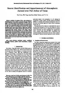
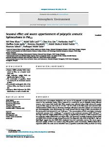
(RSNO3P) at the Welby site. Both simulated and measured agreement are reasonable for many of the samples, but there are some notable deviations. Most of these deviations from the SGS measurements are the same for the SFS and SCAPE nitrate concentrations. There are large and numerous discrepancies corresponding to the samples between 01/15/97 and 01/19/97 that cause these SGS measurements to be suspect at Level 3 validation. Several of the other cases are due to very low nitrate concentrations during one or more of the three-hour periods that possessed large uncertainty intervals. Samples were excluded from SCAPE simulations when simultaneous particulate nitrate concentrations measured by the SGS and SFS failed to agree within two times the uncertainty intervals of both measurements. Table C.2-1 identifies the samples that were removed by this process. The total number of remaining samples to which SCAPE was applied was 110. The second evaluation test involved a comparison between simulated and measured particle nitrate, which is shown in Figure C.2-2. This comparison shows good agreement between simulation and measurements with some disagreement for most of the samples, but there are a few outliers that were identified and investigated further with sensitivity studies. The third evaluation test examined the sensitivity of gas/particle partitioning to possible changes in temperature and relative humidity over the three-hour sampling period. SCAPE results can be influenced by relative humidity and temperature, which affect the amount of liquid water present. Temperature can also influence SCAPE results owing to the temperature dependence of the thermodynamic constants. Of the 110 samples in Figure C.2-2, 56 SCAPE particulate nitrate concentrations differed from SGS measured concentrations by more than twice the measurement uncertainty. For each of the 56 cases, five SCAPE calculations were executed using relative humidity and ambient temperature values for each of the three hours within the 3-hour measurement averages, plus the hour before and the hour after the 3-hour interval. SCAPE-calculated particulate nitrate was within two measurement uncertainty intervals for five of 56 samples for at least one of these equilibrium calculations. The fourth evaluation test examined the sensitivity of gas/particle partitioning to uncertainties in ambient concentration measurements. For each of the 51 remaining samples, SCAPE was applied to eight data sets that systematically added or subtracted twice the reported measurement uncertainty to the total ammonia, total nitrate, and sulfate concentrations. Other input variables were retained at their measured amounts. Twenty-five of the 51 remaining samples yielded particulate nitrate concentrations (for at least one of the eight perturbed data sets) that agreed with measured particle nitrate within two measurement uncertainty intervals. Particulate nitrate concentrations from the SGS and SFS measurements are presented in Table C.2-2 with SCAPE nitrate concentrations, measured temperature, and measured relative humidities for the 26 remaining samples. Table C.2-2 shows that most of the

C.2-4

SCAPE-calculated and SGS-measured particle nitrate concentrations do not differ by more than a factor of two. Nine of these samples show more than a factor of two difference. In three of these cases, the SCAPE-calculated nitrated underestimated the measured nitrate. Relative humidity was low in each of these cases, and SCAPE estimated that no liquid water was associated with the nitrate. SCAPE may underestimate particulate nitrate because it underestimates liquid water. There is experimental evidence for the presence of metastable liquid water on ammonium sulfate particles for relative humidities down to approximately 30% (Tang, 1980) and on aerosol particles in the atmosphere for relative humidities down to approximately 45% (Rood, 1989). In six of the nine cases, SCAPE overestimates particulate nitrate. Some of this overestimation may be due to ammonium nitrate volatilization in the SGS for these samples. Particle nitrate is separated from gas-phase nitrate by passing the aerosol stream through a denuder tube, which removes gas phase HNO3 by diffusion to the denuder tube walls. Since the gas-phase vapor pressure is thus artificially reduced, the equilibrium conditions will tend to move nitrate from the particulate phase to the gas phase where it will be carried to the walls of the denuder.

C.2-5

Table C.2-1 Summary of Level-3-Suspect Three-Hour Sequential Gas Sampler Nitrate Concentrations

Start

SGS Nitrate

SFS Nitrate

SCAPE Nitrate

Date Hour (MST)

(µg/m 3)

(µg/m 3)

(µg/m 3)

0.3 0.2 0.1 0.7 1.3 0.3 3.8 1.1 0.5 0 0.5 0.4 0.7 2.5 0.3 1.3 0.1 0.3 0.6 3.6 5.5 0.6 0.4 0.8 0.5 1.3 0.7 0.6 1.2 1.5 1.7 1.3 0 0 0.1 0 0 0 0 0 0.4 0.7 1.1 0.9 0.5 0.3 0.8 0.4 6.6 0.2 0.9 2.5 0.7

1.3 1.3 0.2 2.8 2.8 2.1 9.2 3.9 1.3 1.3 6.7 1.5 2.6 1 1 9.3 9.3 1.3 1.3 1.3 2.3 2.3 2.3 1.9 1.2 2.8 1.6 1.6 2.6 7.9 7.7 6.2 6.2 4.1 4.1 1 1 10.4 10.4 8.7 6.2 3.4 3.4 1.9 1.2 1.2 2.3 2.3 2.7 2.7 2.7 5.8 1.6

1.3 0.5 0 1.7 1.2 1 18.6 1.1 1.1 1.6 0.4 0.6 3.9 3.5 0.9 1.1 0.8 0.9 1.3 4.5 4.4 0.7 0.6 0 0.5 1.7 0.8 0.9 1.4 6.5 9.8 9.9 2.7 4 2.9 0 4.5 3.7 10.5 7 0.2 0 3.6 2.8 1.5 0 0.7 0 6.8 0.2 1.2 3.3 1.2

Sample Site BRIGHT BRIGHT BRIGHT BRIGHT BRIGHT BRIGHT BRIGHT BRIGHT BRIGHT BRIGHT BRIGHT BRIGHT BRIGHT BRIGHT BRIGHT BRIGHT BRIGHT BRIGHT BRIGHT BRIGHT WELBY WELBY WELBY WELBY WELBY WELBY WELBY WELBY WELBY WELBY WELBY WELBY WELBY WELBY WELBY WELBY WELBY WELBY WELBY WELBY WELBY WELBY WELBY WELBY WELBY WELBY WELBY WELBY WELBY WELBY WELBY WELBY WELBY

12/18/96 12/20/96 12/25/96 12/27/96 12/27/96 1/7/97 1/14/97 1/15/97 1/15/97 1/15/97 1/18/97 1/18/97 1/19/97 1/19/97 1/19/97 1/20/97 1/20/97 1/20/97 1/30/97 1/30/97 12/19/96 12/20/96 12/20/96 12/20/96 12/25/96 1/6/97 1/7/97 1/7/97 1/8/97 1/13/97 1/13/97 1/14/97 1/14/97 1/14/97 1/15/97 1/15/97 1/15/97 1/17/97 1/17/97 1/17/97 1/18/97 1/18/97 1/18/97 1/19/97 1/19/97 1/19/97 1/21/97 1/21/97 1/28/97 1/28/97 1/29/97 1/29/97 1/30/97

6 3 6 0 3 3 9 3 6 9 3 6 6 12 15 0 3 6 6 9 18 0 3 6 6 6 0 3 0 15 18 12 15 18 0 6 9 6 9 12 3 6 9 9 12 15 0 3 18 21 0 6 6

C.2-6

Table C.2-2 Remaining Discrepencies between SCAPE-Calculated and Filter Pack (SGS)-Measured Nitrate Concentrations Sample Site BRIGHT WELBY WELBY WELBY BRIGHT WELBY WELBY BRIGHT WELBY BRIGHT BRIGHT BRIGHT BRIGHT BRIGHT BRIGHT BRIGHT BRIGHT BRIGHT BRIGHT BRIGHT BRIGHT BRIGHT BRIGHT BRIGHT BRIGHT BRIGHT

Start

Date Hour (MST) 12/25/96 12/20/96 1/15/97 1/30/97 12/19/96 1/14/97 1/13/97 2/3/97 1/18/97 12/20/96 1/13/97 1/14/97 1/13/97 2/3/97 1/14/97 2/2/97 12/18/96 1/29/97 1/19/97 1/28/97 1/20/97 2/2/97 1/21/97 1/29/97 1/28/97 1/20/97

15 9 3 9 6 21 21 3 0 0 15 15 12 0 12 21 15 0 9 6 9 18 0 3 21 12

SCAPE Nitrate 3

SGS Nitrate 3

SCAPE/ SGS

Temp.

RH

Water 3

(µg/m )

(µg/m )

Ratio

°C

%

(µg/m )

0 0 0.3 1.42 1.81 4.43 3.94 2.49 3.1 0.96 9.74 2.75 6.25 4.95 12.01 4.9 1.25 2.9 4.54 2.6 3.76 4.64 1.29 5.16 3.92 6.51

1.15 2.92 4.79 2.73 3.26 7.54 6.68 3.72 4.35 0.7 7.03 1.95 4.23 3.17 7.51 2.83 0.72 1.57 2.42 1.37 1.72 2.07 0.55 2.17 1.12 1.85

0 0 0.0626 0.5201 0.5552 0.5875 0.5898 0.6694 0.7126 1.3714 1.3855 1.4103 1.4775 1.5615 1.5992 1.7314 1.7361 1.8471 1.876 1.8978 2.186 2.2415 2.3455 2.3779 3.5 3.5189

7.3 1.9 0.5 6.6 -13.2 -7.8 -17.7 -0.5 -2.2 -8 -18.5 -9.5 -18.4 -1.3 -10.2 -0.3 -11.2 3.5 2.7 -8.1 5.9 3.2 3.8 2.3 3.8 13.8

31.8 37.8 37.8 31.2 71.4 87.1 69.2 83.1 63.5 60.7 73.7 85.9 73.6 85.5 82.2 82 50.9 43.4 62.7 82.6 53.4 70.9 55.8 78.2 37.9 39.3

0 1.03 0 0 3.84 23.01 5.88 4.98 2.07 0 13.98 13.01 10.15 12.09 27.23 10.21 0.86 0 3.31 6.72 0.03 5.13 0 7.29 0 0

C.2-7

Figure C.2-1.

Ratios of simulated particle nitrate to SGS particle nitrate (RSNO3P) and SFS particle nitrate to SGS particle nitrate (RNO3P) for samples taken at the Welby site. Major deviations from unity occur for both ratios on the same samples, indicating inaccuracies in the corresponding SGS measurements.

Modeled Particle Nitrate (ug/m3)

20

0 0

20 Measured Particle Nitrate (ug/m3)

Figure C.2-2.

Comparison of simulated and measured particulate nitrate for 110 samples at the Welby and Brighton sites. C.2-8

C.3

TRANSPORT SIMULATIONS

Transport simulations were undertaken to determine the possibilities of air movement between identified emissions sources and NFRAQS receptors. This section explains how the transport simulations were applied, the input data that were used, and their sensitivity to measurement uncertainties and deviations from simulation assumptions. C.3.1

CALMET, UAM, and SCIPUFF Formulation and Software

The CALMET meteorological simulator consists of a diagnostic wind field module and micro-meteorological modules for over-water and over-land boundary layers (EPA, 1995). The Urban Airshed Model (UAM) uses these windfields to simulate the movement of air between adjacent grid squares and layers. The CALMET diagnostic module uses a two-step approach (Douglas and Kessler, 1988). In the first step, an initial-guess field is adjusted for kinematic effects of terrain, slope flows, and terrain blocking effects. The second step consists of an objective analysis procedure to introduce observational data into the Step 1 wind field to produce a final wind field. Options are provided to use gridded prognostic wind fields as: 1) the initial guess; 2) the Step 1 wind field; or 3) as “observational data”. Prognostic simulations follow the time evolution of the atmospheric system through the space-time integration of the equations for conservation of mass, motion, heat, and water. Over land surfaces, an energy balance method is used to compute hourly gridded fields of the sensible heat flux, surface friction velocity, Monin-Obukhov length, and convective velocity scale. Mixing heights are determined from the computed hourly surface heat fluxes and observed temperature soundings. Gridded fields of Pasquill/Gifford/Turner stability class and optional precipitation rates are also determined by the simulation. CALMET contains two principal sub-modules: The Diagnostic Wind Module (DWM) and the Micro-Meteorological Module (MMM). As with all simulations of complex phenomena, each module has significant limitations with respect to representing the real world. Limitations of the diagnostic wind module are: •

While CALMET solves the incompressible mass continuity equation, the method does not explicitly conserve momentum or energy as in prognostic simulations.

•

Reliability of the interpolated fields in the diagnostic wind module improves as the measurement density increases; conversely, reliability degrades where measurements are sparse.

•

Experience has shown that these simulations are not reliable under light wind situations, highly stable or unstable conditions, and situations with significant vertical wind variations.

C.3-1

Limitations of the micro-meteorological module are: •

Micro-meteorological parameters are calculated by CALMET based on parameterizations that include many variables. Error derives from limitations in the input data, for which direct measurements are sparse or unavailable. Complex terrain greatly exacerbates this problem.

•

CALMET does not include an adjustment of sun angle to account for the total terrain slope. As a result, the simulation does not properly account for differential heating of mountain slopes that can produce significant stability, mixing height, and wind direction differences over surfaces with different orientations relative to the sun.

Given these limitations, several atmospheric processes in the NFRAQS domain may not be quantitatively simulated with CALMET. Inaccurate lapse rates and uncertainties in the estimated micro-meteorological variables lead to inaccuracies in daytime convective mixing height. This is of particular concern for the NFRAQS simulations owing to the position of elevated point source plumes near the top of the surface mixed layer. Uncertainties of the mixed layer depth can result in large inaccuracies in estimates of plume location and dispersion. In the Mt. Zirkel Visibility Study in northwestern Colorado (Watson et al., 1996), however, it was found that the CALMET mixing depth estimates compared well with those determined by radar profiler measurements when such vertical, remote sensing data were available. The CALMET was applied to six NFRAQS Winter 97 episodes: 1) 01/11/97 0000 MST to 01/21/97 0600 MST; 2) 01/27/97 0000 MST to 01/31/97 0600 MST; 3) 12/30/96 0000 MST to 01/03/97 0600 MST; 4) 12/18/96 0000 MST to 12/20/96 1200 MST; 5) 12/25/96 0000 MST to 12/27/96 0600 MST; and 6) 02/01/97 0000 MST to 02/05/97 1800 MST. These simulations yielded estimated wind speeds and directions at many locations and elevations as well as surface mixing depths into which pollutants were released, combined, and reacted. These wind field simulations were used to estimate where concentrations at receptors came from, and to simulate the transport and dispersion of emissions from selected sources and source areas. The horizontal domain for CALMET covered an area of 312 km (east-west) by 220 km (north-south), as shown in Watson et al. (1998). A UTM-grid was used with UTM zone 13 to specify the horizontal coordinates. The south-west corner of the grid lies at 435 km easting and 4320 km northing. The horizontal grid size used was 4 km x 4 km. The height of the highest layer was 2800 m above ground level (agl), and this contained 26 vertical layers. The first vertical cell thickness was 20 m agl, and the second cell thickness was 30 m. For the other vertical cells, 50-m-thick cells were used to 1 km height agl, 250-m-thick cells were used from 1 to 2 km agl, and the highest cell had a thickness of 800 m. This arrangement of vertical cells was used to be consistent with the vertical structure used in the gridded transport simulations.

C.3-2

CALMET reads a “control file” that specifies selections for the control options, input variables, and outputs. Diagnostic Wind Module (DWM) parameters are the most important in controlling the final wind fields generated using CALMET. Table C.3-1 shows the selection of options for this application and compares them with the default recommendations. The gridded transport simulations were performed using UAM-IV. UAM-IV is an urban-scale three-dimensional photochemical air quality simulator that is most often used to simulate the evolution of ozone and other photochemical pollutants in an urban environment. For this study, the UAM-IV was applied to estimate the dispersion of primary emittants (SO2 and NOx) from different emitters and source areas using the CALMET meteorological outputs. The purpose of these simulations was to determine the sulfur dioxide and oxides of nitrogen emitters that most probably arrived at NFRAQS receptors. Just as important, these simulations determined which emitters did not provide minor, moderate, large, or major contributions to these precursors at NFRAQS receptors. These simulations were not intended to, and were not used to, estimate contributions to PM2.5 ammonium sulfate and ammonium nitrate concentrations. They were used to eliminate certain emitters as direct and short-term contributions to secondary sulfates and nitrates at NFRAQS receptors. The horizontal domain for UAM-IV transport simulations was the same as that described above for CALMET. The grid size used was 4 km x 4 km, which was also the same as used in the CALMET. Layers up to 2000 m agl were included. Twenty-four layers were included in the simulation, 20 below the diffusion break (diffbreak) and four above the diffusion break. The diffusion break is the turbulent mixing depth during neutral/unstable conditions and the depth of the surface based inversion during stable conditions. A minimum vertical cell height of 50 m, and a maximum vertical cell height of 250 m was used. This arrangement of vertical cells forces constant vertical levels with first 20 cells from bottom of 50 m thickness, and 4 top cells of 250 m thickness. This arrangement of vertical cells avoided a moving mesh (that can create pseudo-vertical velocities), and allowed high-resolution near the ground. The puff transport simulations were performed using the Second-order Closure Integrated Puff (SCIPUFF) simulator (Sykes and Gabruk, 1997). SCIPUFF simulates the plume concentrations downwind of a power plant stack. It represents the plume as superposition of a series of Gaussian puffs, typically 10 seconds apart. Puffs spread as they move downstream. To eliminate unnecessary overlap and to maintain a manageable number of puffs, a merging algorithm is used. SCIPUFF uses a variable time-step algorithm which allows small time-steps at the stack exit. It also uses small spatial scales at the stack exit and larger scales away from the source. This allows an efficient computation of the wide range of scales involved in the stack emission problem. SCIPUFF requires three-dimensional winds, three-dimensional temperatures, 2-dimensional mixing heights, 2-dimensional stability classes, and 2-dimensional heat flux. The horizontal domain used in the SCIPUFF was the same as that used in CALMET and UAM-IV. All the inputs required by the SCIPUFF were calculated using CALMET. Heat flux parameter is calculated by CALMET at the measurement stations, and not for the whole

C.3-3

grid. The heat flux calculated at the Brighton site was used for the whole grid in SCIPUFF as there was no significant variation from station to station. SCIPUFF was run from 01/13/97 to 01/20/97, separately for three different power plants (Cherokee, Pawnee and Valmont). A stack parameter file was prepared for each power plant stack. This file includes the coordinates for the point of release, the amount of release, and the time and duration of the release. A series of releases were used at hourly intervals with a duration of 1 hour each to input the hourly varying emissions. Horizontal coordinates of the point of release were calculated from the location of the power plant. The vertical point of release was calculated as sum of the stack height and the plume rise. Plume rise was calculated using algorithm used in the CALPUFF simulator that uses Briggs formula and equations with wind shear effects to calculate the plume rise. Computer animations were prepared to display the results of both the gridded and puff transport simulations. These simulations were used to visualize potential transport of elevated and surface sulfur dioxide emissions. The base map in the animations is highly simplified. The boundaries of the display are the boundaries of the domain, and only the locations of the core sites and some of the major point sources are shown. The animations show the transport and dispersion of SO2 for nine source groupings. The final character is a number that indicates one of nine different SO2 sources: 1) Arapahoe coal-fired power station elevated stack; 2) Cherokee coal-fired power station elevated stack; 3) Pawnee coal-fired power station elevated stack; 4) Valmont coal-fired power station elevated stack; 5) Rawhide coal-fired power station elevated stack; 6) Trigen coal-fired power station elevated stack; 7) Conoco and Diamond Shamrock refineries combined; 8) other elevated sulfur emitters combined; and (9) surface sulfur emitters combined. Separate animations were prepared for surface concentrations and vertically integrated burdens. The vertically integrated burdens indicate the location of the emissions without regard to their height above ground level. There are separate animations for each source individually for both the surface and vertically integrated concentrations and also animations that show the surface and vertically integrated concentrations due to all sources combined. The computer files containing the animations are part of the NFRAQS database. The files from the gridded transport simulations have seven character names and an “avi” extension. The first five characters are the month and day of the start of the animation (e.g., jan11). The next character is “s” when the simulation shows the sulfur concentration in the surface layer and “i” when the simulation shows the vertical integration of all sulfur at all heights in that grid cell. Surface sources included mobile, area, and wood burning emissions as well as emissions from point sources with stacks less than 30 m (100 ft) high. Trigen includes more than one unit at the Coors brewery. If the final character is missing in the file name, the animation shows the sum of the concentrations from the separate sources. Files from the puff transport simulation are named “Cher-13s.avi”, “Valm-13s.avi”, and “Pawn-13s.avi”, and show surface concentrations from Cherokee and Pawnee beginning 01/13/97. In all simulations, the color scale is logarithmic. Base-10 logarithm of

C.3-4

concentration are calculated and mapped to a linear color ramp from blue at the lowest concentrations to red at the highest concentrations. If the value is less than the minimum threshold, it is assigned the color black. If the value is greater than the maximum threshold, it is assigned the color white. For the surface data the minimum threshold is 0.2 ppbv and the maximum threshold is 100 ppbv. For the vertically integrated data the minimum threshold is 0.1 ppmv/m and the maximum threshold is 30.0 ppmv/m. Movie4.exe and three “dll” files are freeware from Lantern Corporation that can be used to view the animations, as can movie software available with Windows 95. To use this viewer, copy these files to the same directory as the “avi” files. From Windows Explorer, double click on Movie4. Click at the upper left of the window that opens and choose Options/Control/Remote. Drag the Remote window to a convenient place (e.g., the lower right corner of the screen). Click Open, and select the “avi” file to be viewed. The Remote can be used to view single frames, change the speed of the display, etc. It is possible to open a second Movie4 and display two animations side-by-side. C.3.2

CALMET and UAM Input Data

C.3.2.1

CALMET Data

CALMET requires surface meteorological measurements, upper air meteorological measurements, and geophysical measurements. C.3.2.1.1 Surface Data CALMET requires hourly surface observations of wind speed and direction, temperature, cloud cover, ceiling heights, surface pressure, relative humidity, and optional precipitation type codes which are used only if wet removal is to be simulated. Most routine sites report only wind and temperature data. The NFRAQS data base (Chow et al., 1998) contains a large number of surface meteorological measurements from a variety of networks. Eight National Weather Service (NWS) stations recorded wind, temperature, relative humidity, solar and net radiation. Some NWS stations also reported pressure, cloud cover and ceiling height data. Seven Remote Automated Weather Stations (RAWS) reported temperature, winds and relative humidity. Thirty-four stations from a variety of networks recorded in the Aerometric Information Retrieval System (AIRS) reported winds and temperature. Twelve Colorado Agricultural Meteorological Stations (COAGMET) reported temperature, winds and relative humidity. Surface meteorological measurements (winds, temperature and relative humidity) were also acquired from NFRAQS monitors collocated with NFRAQS upper air measurements. CALMET allows missing values, but at least one surface site should have a valid data for each hour. A screening program developed for NFRAQS takes the surface data from different networks and creates a single data file which can be directly used by the CALMET simulator. C.3.2.1.2 Upper Air Data CALMET uses wind speed, wind direction, temperature, and pressure measurements C.3-5

at different elevations above ground level. At least one station provides these data with a minimum of two vertical measurements per day. Vertical pressure measurements, however, are not essential. Six NFRAQS radar profilers that measured wind speed and direction from 100 m agl to 2000 to 4000 m agl, depending on weather conditions. Radio-Acoustic-Sounding-Systems (RASS) measured virtual temperature from 100 m agl to ~800 m agl. Twice-daily soundings from the NWS site at Denver International Airport were also available. Doppler sodar systems at Welby reported high-resolution (10 m) wind data from about 50 to 200 m. Vertical meteorological measurements are needed below the 100 m agl lower limit or the radar profilers. Surface measurements were merged with the upper air measurements in an integrated CALMET input data file. Where nearby surface measurements were lacking, radar profiler measurements were extrapolated to the surface with a power-law formula. Similarly, missing data at the top of the domain were filled with the closest available profiler measurements. RASS reports temperature data to about 800 m from the ground. Temperatures were extrapolated above 800 m agl by assuming a wet adiabatic lapse rate. C.3.2.1.3 Geophysical Data Geophysical data include terrain elevations, land uses, roughness length, Bowen ratio, soil heat flux, and leaf area index averaged over the 4 km x 4 km grid squares. Roughness lengths, Bowen ratios, soil heat fluxes, and leaf area indices are constants related to land use, obtained from the United States Geological Survey (USGS) Land Use and Land Cover digital data base (Watson et al., 1998). These data provide information on nine major land use classes, with 37 subclasses, and are available in Composite Theme Grid (CTG) format with a resolution of 200 meters (defined in local UTM coordinates). The USGS 3-arc second Digital Elevation Models (DEM) are used for terrain elevations. Three-arc second DEMs yield a resolution of approximately 70 m in the east-west direction and 90 m in the north-south direction. Each terrain height is assigned to the appropriate grid cell, after converting the data locations to the grid coordinates, and an arithmetic average terrain height is calculated for each grid cell. When no valid data were available in the NFRAQS data base at any site for a particular variable and hour, default values were assigned. These defaults are: 1) 273 °K for temperature; 2) 800 mb for pressure; 3) 99,000 ft for ceiling (unlimited); 4) zero for skycover; 5) 1 m/s for wind speed; and 6) 20% for relative humidity. The only variables for which the default values were needed were for skycover and ceiling height. For all other variables there was at least one site with the valid data. Several inconsistencies between CALMET input data requirements and NFRAQS data were addressed by the following: •

NFRAQS profilers report only virtual temperature at upper levels. The difference between the surface air temperature and surface virtual temperature was added to the virtual temperature at upper levels to obtain absolute upper air temperatures.

C.3-6

•

The following algorithm extended profiler wind measurements above their highest level to the top of the domain. ZTOP denotes the highest elevation reported by the radar profiler for a particular hour. MTOP denotes the top of the domain. − When ZTOP exceeded 1500 m agl, MTOP=ZTOP. − When ZTOP