242
IEEE TRANSACTIONS ON AUDIO, SPEECH, AND LANGUAGE PROCESSING, VOL. 19, NO. 2, FEBRUARY 2011
Source–Filter-Based Single-Channel Speech Separation Using Pitch Information Michael Stark, Student Member, IEEE, Michael Wohlmayr, Student Member, IEEE, and Franz Pernkopf, Member, IEEE
Abstract—In this paper, we investigate the source–filter-based approach for single-channel speech separation. We incorporate source-driven aspects by multi-pitch estimation in the model-driven method. For multi-pitch estimation, the factorial HMM is utilized. For modeling the vocal tract filters either vector quantization (VQ) or non-negative matrix factorization are considered. For both methods, the final combination of the source and filter model results in an utterance dependent model that finally enables speaker independent source separation. The contributions of the paper are the multi-pitch tracker, the gain estimation for the VQ based method which accounts for different mixing levels, and a fast approximation for the likelihood computation. Additionally, a linear relationship between pitch tracking performance and speech separation performance is shown. Index Terms—Single-channel speech separation (SCSS), multipitch estimation, source–filter representation.
I. INTRODUCTION HE aim of source separation is to divide an instantaneous of two signals into its unlinear mixture derlying source signals and . For single-channel speech separation (SCSS) two sound sources are mixed into a single channel. This is in general an ill-posed problem and cannot be solved without further knowledge about the sources or their interrelationship. SCSS can be mainly divided into the area of implicit models also known as computational auditory scene analysis (CASA) and explicit models known as underdetermined blind source separation methods [1]. Implicit models try to mimic the remarkable ability of the human auditory system to recover individual sound components in adverse environments. Here, the mixture is a scene to be organized and particular extracted components are merged to form output streams of individual sources. The CASA systems in [2] and [3] are the most important representatives. Both systems are heavily based on harmonicity as cue for separation. Wang et al.
T
Manuscript received August 31, 2009; revised December 17, 2009; accepted February 25, 2010. Date of publication April 05, 2010; date of current version October 27, 2010. This research was carried out in the context of COASTROBUST, a joint project of Graz University of Technology, Nuance Communications International, and Sail Labs Technology. This work was supported by the Austrian KNet Program, in part by the ZID Zentrum for Innovation and Technology, Vienna, in part by the Steirische Wirtschaftsfoerderungsgesellschaft mbh, in part by the Land Steiermark, and in part by the Austria Science Fund under Project P19737-N15. The associate editor coordinating the review of this manuscript and approving it for publication was Dr. Sharon Gannot. The authors are with the Signal Processing and Speech Communication Laboratory, Graz University of Technology, Graz 8010, Austria (e-mail: michael.
[email protected]). Color versions of one or more of the figures in this paper are available online at http://ieeexplore.ieee.org. Digital Object Identifier 10.1109/TASL.2010.2047419
[4], [5] suggested the use of the ideal binary mask as computational goal for auditory scene analysis. The ideal binary mask uses the mixture maximization (mixmax) approach [6], i.e., the element-wise maximum operator applied on a time–frequency representation, i.e., the spectrogram, to separate the two signals. In contrast, explicit models incorporate prior knowledge such that the individual source characteristics are learned in a generative manner during a training phase. This speaker-dependent model is used as source prior knowledge and is applied for separation without considering the interfering component. The two most prominent explicit models are the factorial-max vector quantization [7] (VQ) and the factorial-max hidden Markov model [8] which also integrates time dependencies. In both models, the most likely states at every time instance are selected in the mixmax sense, conditioned on the observed mixture. Another method capable of identifying components with temporal structure in a time–frequency representation is non-negative matrix factorization (NMF) [9], [10]. Here, the mixture is decomposed into a bases and a weight matrix. The weight matrix specifies the contribution of each basis to model the observation. The layered factorial HMM in [11] is currently the best performing method on the Pascal Speech Separation Challenge [12]. To model speaker characteristics, an acoustic model which is driven by a grammar model is used. Only for the grammar model a first-order Markov process is employed. However, in this work speech recognition of mixed signals is the main task. In this paper, we use the source- and model-driven approach as already proposed by Radfar et al. [13]. They suggest to also consider the speech signal characteristics and use them as an additional cue for separation. Using this as a basis, the signal can be decomposed into a fine spectral structure related to the excitation signal and a coarse spectral structure representing the vocal tract information. The source-driven part extracts the fundaor its perceived counter part, the pitch inmental frequency formation of each speaker using a multi-pitch tracking method. Afterwards, the estimated pitch of each speaker is used to synthesize an artificial excitation signal representing the fine spectral structure. Utilizing this excitation signal, the vocal-tract filters (VTFs) are estimated based on a probabilistic model-driven approach. This decomposition results in a speaker independent (SI) system in contrast to most other methods, e.g., [7], [10], and [11]. For both, the multi-pitch estimation algorithm and the VTF estimation method we used the same time–frequency representation, i.e., the spectrogram. An approach for robust multi-pitch tracking has been proposed in [14]. It is based on the unitary model of pitch perception
1558-7916/$26.00 © 2010 IEEE
STARK et al.: SOURCE–FILTER-BASED SCSS USING PITCH INFORMATION
243
[15], upon which several improvements are introduced to yield a probabilistic representation of the periodicities in the signal. Semi-continuous pitch trajectories are then obtained by tracking these likelihoods using an HMM. Although this model provides an excellent performance in terms of accuracy, it is not possible to correctly link each pitch estimate to its source speaker. Recently, it was shown that factorial HMMs (FHMMs) [16] provide a natural framework to track the pitch of multiple speakers [17], [18]. In this paper, we go a step further and use Gaussian mixture models (GMMs) to model the spectrogram features of the speech mixture. For this purpose, we require supervised data, i.e., the pitch-pairs for the corresponding speech mixture spectrograms to learn the GMMs. These data are generated from single speaker recordings applying the RAPT pitch tracking method [19]. Learning the GMMs is combined with the minimum description length (MDL) [20] criterion to find the optimal number of Gaussian components for modeling the spectrograms belonging to a specific pitch-pair. This approach significantly outperforms two methods based on correlogram features. We report these results in [21]. For the coarse spectral structure, a speaker independent VTF model is trained. Therefore, we compare two statistical methods, one is based on VQ and the other one on NMF. Additionally, we propose a new gain estimation method for the VQ model addressing the problem of different mixing levels. Furthermore, we propose a computational efficient method for the likelihood estimation. This method is in spirit similar to beam search [22] used for efficient decoding in HMMs. To evaluate these methods, we assess performance in various ways using the Grid Corpus [12]. First, results are reported for every single building block, i.e., the multi-pitch tracking algorithm, the gain estimation, and the likelihood approximation. Second, separation performance on the SCSS task is assessed extracting pitch information in a speaker-dependent (SD), gender-dependent (GD), and finally speaker-independent (SI) way. Moreover, we perform separation using reference single pitch trajectories taken from RAPT. Third, we present performance results using just the excitation signals for speech separation. The remainder of this paper is structured as follows. In Section II, we introduce the general model for the source–filter-based SCSS. Section III presents the multi-pitch tracking algorithm. The proposed VTF models are characterized in Section IV. The experimental setup and results are discussed in Section V. Finally, we conclude and give future perspectives in Section VI.
II. SOURCE- AND MODEL-DRIVEN APPROACH In the source–filter model, the speech signal is composed of an excitation signal that is shaped by the vocal tract acting as a filter process. Hence, a speech segment is the convolution of which are further multiplied the excitation with the VTF by a gain factor in the time domain as (1)
Fig. 1. Blockdiagram of the separation system.
. The convolution where the speaker index is given as results in a multiplicative relation in the frequency domain as
Generally, we denote signals in time domain in lower case, e.g., and , signals in the magnitude spectral domain by uppercase and , and signals in the characters with a half-pipe, e.g., and log-magnitude spectrum in uppercase only as throughout the paper. The overall SCSS system is shown in Fig. 1 and consists of the following building blocks: a multi-pitch tracking unit followed by the excitation generation unit is representing the source-driven part. In this paper, we compare SD, GD, and SI multi-pitch tracking performance and employ them for speech separation. Once the pitch trajectories of each speaker are estiand , they are further utilized to create the exmated, i.e., and . Details about the source-driven part citation signals are described in Section III. VTFs, known as spectral envelopes, and are used to train are extracted from SI training data , either a or a model (see Section IV). SI models and the VTF model The combination of the excitation signal which is carried out in the model combination block of Fig. 1, re, i.e., the VTFs sults in an utterance dependent (UD) model in combination with the excitation are modeling a particular utterance. Thus, the harmonic excitation signal acts as discriminative feature and introduces utterance dependency which enables speech separation. The UD model is further used to separate the speech mixture in the separation step. For performance analysis we can estimate the component signals in two ways. • The most likely speech bases of each component speech signal are used to find the respective binary masks (BMs). Afterwards, the BM is used to filter the speech mixture in order to get an estimate of the component signal . • The estimated speech bases are directly used for synthesis of the component speech signals . In the reconstruction block of Fig. 1, the separated speech signals are synthesized by first applying the inverse Fourier transform on each speech segment using the phase of the . For speech signal reconstruction the mixed speech signal overlap–add method is used.
244
IEEE TRANSACTIONS ON AUDIO, SPEECH, AND LANGUAGE PROCESSING, VOL. 19, NO. 2, FEBRUARY 2011
A. FHMM Parameters The state-conditional observation likelihoods are modeled with a GMM using components according to
Fig. 2. Factorial HMM shown as a factor graph [23]. Factor nodes are shown as shaded rectangles together with their functional description. Hidden variable nodes are shown as circles. Observed variables are absorbed into factor nodes.
X
In this paper, we use different models to represent certain speaker spaces. The SI space is characterized by one universal model valid for all speakers and phonemes they can articulate. The GD model is trained to represent the distribution unique for each gender, male or female. Further, the SD model describes the space of each individual speaker. A subset of the SD space is the utterance dependent space, i.e., an individual model per utterance. Hence, the SI space can be decomposed according GD SI. to: UD III. MULTI-PITCH TRACKING USING FHMM We use an FHMM for tracking the pitch trajectories of both speakers. The FHMM represented as factor graph [23] is shown in Fig. 2. The hidden state random variables are denoted by , where indicates the Markov chain related to the speaker index and the time index from 1 to . Similarly, the observed random variables, i.e., the log magnitude specat time . Each represents a discrete trum, are denoted by is random variable related to the pitch of speaker at , while continuous. For simplicity, all hidden variables are assumed to have cardinality . The edges between nodes indicate a conditional dependency between random variables. Specifically, the dependency of hidden variables between two consecutive time instances is defined for each Markov chain by the transition . The dependency of the observed variprobability ables on the hidden variables of the same time frame is de. Finally, the fined by the observation probability prior distribution of the hidden variables in every chain is de. Denoting the whole sequence of variables, i.e., noted by and , the joint distribution of all variables is given by
The number of possible hidden states, i.e., per time frame is . As pointed out in [16], this could also be accomplished by an ordinary HMM. The main difference, however, is the constraint placed upon the transition structure. While an HMM with states would allow any transition matrix between two transition hidden states, the FHMM is restricted to two matrices.
To obtain , we first apply the zero padded 1024 point of length 32 FFT on a Hamming windowed signal segment ms. Next, we take the log magnitude of spectral bins 2–65, which corresponds to a frequency range up to 1 kHz. This covers the most relevant frequency range of resolved harmonics while corresponds to the keeping the model complexity low. weight of each component . These weights are and . The constrained to be positive can be learned by parameters the EM algorithm [24], where . states, where state value Each hidden variable has “1” refers to “no pitch,” and state values “2’–‘200” correspond to different pitch frequencies ranging from less than 1 ms to kHz. Note that segments of silence 12.5 ms, i.e., 80 Hz. For learning the and unvoiced speech are modeled by GMM we need supervised data, i.e., the pitch-pairs for the corresponding speech mixture spectrograms. These data are composed from single speaker recordings using the RAPT pitch extraction [19]. Hence, with both pitch trajectories for the mixed utterances at hand, we can easily learn a GMM for each pitch-pair . Accordingly, we have to determine 200 200 GMMs. Unfortunately, data might be rarely available for some pitch-pairs, whereas, there is plenty of data for, e.g., . For this reason, we use MDL to determine the number of components of the GMM automatically. The MDL criterion [20] is
where is the number of parameters per component (for GMMs with diagonal covariance matrix where in our case), in all spectrogram samples belonging to are collected, and denotes the size of , i.e., . This equation has the intuitive interpretation that the log-likelihood is the code length of the encoded data. The term models the optimal code length for all parameters . In for a particular we use a single case of Gaussian with and is set to a small , where is the identity matrix. For , we ranging from 1 to 15, and take the GMM train GMMs with whose corresponding MDL criterion is minimal. If there is , i.e., no training sample available for the pitch-pair , we set and . Prior to pitch tracking all spectrogram samples are normalized to zero mean and unit variance. Finally, we multiply the pitch likelihood with the pitch-pair prior , since this slightly improved the performance in our experiments. are obBoth transition matrices of the FHMM tained by counting and normalizing the transitions of the pitch
STARK et al.: SOURCE–FILTER-BASED SCSS USING PITCH INFORMATION
245
values from single speaker recordings. Additionally, we apply . The prior Laplace smoothing1 on both transitions are obtained in a similar manner. distributions
while a message from factor
to variable
is
(4) B. Tracking The task of tracking involves searching the sequence of that maximizes the conditional distribution hidden states : (2) For HMMs, the exact solution to this problem is found by the Viterbi algorithm. For FHMMs, an exact solution can be found using the junction tree algorithm [25]; however, this approach gets intractable with increasing number of hidden Markov . Algorithms for approximate and exact soluchains and tions on FHMMs are derived in [16]. Approximate inference algorithms are often derived from the framework of variational inference. The sum–product algorithm [23] can be derived under a similar setting of variational principles [26], although more intuitive derivations exist for graphs without loops. When applied on a graph with loops, as is the case for a FHMM, the solutions are in general not guaranteed to converge and can only approximate the optimal solution. In this paper, we explored the max-sum algorithm (a variant of sum-product algorithm) as well as the junction tree algorithm. We apply both variants on the loopy FHMM graph to obtain a solution for (2). In contrast to the junction tree algorithm, the max-sum algorithm can only approximate (2). In [18], experimental results suggested that the obtained solutions sufficiently approximate the exact solution, while computational complexity is much lower. Indeed, the time complexity of the , where max-sum algorithm applied to a FHMM is is the number of Markov chains. In contrast, the time com. plexity of the junction tree algorithm is In the sequel, we give a short overview of the used max-sum message passing algorithm. For a detailed discussion, we refer the interested reader to [23], [25], and [26]. Further, details on the junction tree algorithm are given in [16]. The max-sum algorithm is based on passing messages between nodes of a graph. Among various types of graphs, factor graphs [23] have become popular to depict the mechanisms of message passing. Fig. 2 shows a FHMM as factor graph, where the functional dependency of each variable node, for brevity called , is made explicit by “factor nodes,” shown as shaded rectangles, i.e., each of its adjacent (i.e., neighrectangle denotes a function . boring) variable nodes For the max-sum algorithm, each node sends to every neighbor a vector valued message , which is itself a function , for the case of of the messages it received, (as well as a factor node). A message from variable node to factor node is (3) 1Laplace smoothing amounts to the initialization of each element of the transition matrix with count one, i.e., adding the prior information that each transition was observed at least once. This smooths the transition probabilities.
denotes the set of neighbor nodes of . We normalize Here, each message and restrict each node to send a maximum of 15 messages per link. Further, each node only re-sends a message to a neighbor if it is significantly different from the previously sent message in terms of the Kullback–Leibler-divergence. After the last iteration, we obtain the maximum a posteriori configuraof each variable node as a function of its tion incoming messages according to (5)
Although the set of maxima does not necessarily yield the global maximum , as multiple global maxima might be present, a backtracking stage may lead to inconsistencies due to the loops in the factor graph. For to the set this reason, we simply set the global maximum of individual maxima . C. Excitation Synthesis Once the pitch tracks are estimated for each speaker, the harmonic part of the excitation signal is modeled as
(6) where denotes the number of harmonics up to a specified set to 4 kHz, is in radians of a highest frequency is the phase of the mixed signal, and particular time frame, is the time index in a time frame. at is the sampling frequency divided by , i.e., for . For unvoiced and silent signals, i.e., , all a Gaussian random signal is used as excitation and for voiced signals, a Gaussian random signal filtered by a high-pass with is added to (6). This equation is simcutoff frequency at ilar to the harmonic plus noise model [27] but without amplitude weighting of the harmonics. In our case, this weighting is provided by the VTF estimation algorithm. IV. VOCAL TRACT FILTER MODELS In this section, we propose two different statistical VTF models for speech separation. The first method is based on the maximum-likelihood (ML) estimation of the VQ codewords. Here, the mixture maximization (mixmax) approach [6] is used as combination operator to represent the speech mixture . Moreover, we discuss a gain estimation method to make our separation approach suitable for different mixing levels. Finally, we restrict the search space of the VQ to the most promising codewords by applying beam search. Second, we use NMF to model the VTFs.
246
IEEE TRANSACTIONS ON AUDIO, SPEECH, AND LANGUAGE PROCESSING, VOL. 19, NO. 2, FEBRUARY 2011
posteriori (MAP) estimate has to be computed. The MAP can be found by Bayes theorem using (9) as
(10)
Fig. 3. Factorial-max VQ where and S .
X
and are assumed to be independent prior diswhere tributions. Thus, the most likely states can be found by is represented by two state variables S
A. Maximum-Likelihood-Based Source Separation
(11) Assuming uniform priors
The speech mixture is approximated in the log magnitude–frequency domain by the conditional probability distribution model as (7) and are the speech mixture and the respective where underlying speech signals and is the normal distribution. For the separation of the speech signals, we rely on the sparse nature of speech in its high-resolution time–frequency representation. Therefore, the mixmax operator is employed to combine and in order to represent the obserthe hidden variables vation . Hence, the log-spectrum of a mixed signal can be approximated by the element-wise maximum of the log-specand : . trum of the component signals This leads to the notion of the binary mask (BM). A “1” in the BM assigns the corresponding time–frequency cell to speaker one, whereas the cell is allocated to speaker two in case of a “0.” The binary masks of two speakers are complementary, i.e., BM . The observation model in (7), where two hidden BM variables explain an observation is called a factorial-max VQ model illustrated in Fig. 3. Now, given the speaker dependent models and assuming that we have access to the state sequence chosen by the latent variables and associated with each speaker, the joint distribution of the observation and the underlying source signals for a particular instant of time is given as (8) of speaker . where is associated with a particular basis given the Finally, we require the posterior distribution for unobserved hidden variables to model the dependency between and . the speech mixture and the current states This is achieved by marginalization over the underlying signal components as
(9) The aim of source separation is to compute the observation likelihood conditioned on the given state sequences. To form an estimate of the component signals the maximum a
and and neglecting and we can further write . Besides, we assume that the density function conditioned on the states is deterministic and has the following property: if otherwise
(12)
Introducing this assumption in (9) results in the following relation: , where we represent by the basis which has been drawn by the latent variable . This relation directly enables the application of the VQ bases in (7) to separate the speech signals. In the sequel, we introduce the source–filter-based approach for the above framework. To estimate the SI-VTF densities , the training data is split into mutually nonintersecting clusters. These densities are assumed to be Gaussian with a spherical covariance matrix. Hence, we use the k-means algorithm [28] to determine the cluster centers . Thus, the SI VTF model is composed of: . Each codebook entry of the VQ can be thought of representing a prototype VTF. Using this knowledge we can formulate an utterance and , the gain factor dependent VQ by incorporating depending on the basis of speaker as (13) is provided by pitch extraction and the gain factor where is in detail introduced in Section IV-A1. Thus, the UD model can be found by (14)
The UD models are employed for separation. Hence, the most likely bases and representing are selected and used to find the BM or the synthesized signals. To extract the vocal tract filters we use the SEEVOC method described in [29], where the gain information is implicitly included. Hence, for an equal mixing level of the two speech signals the gain factor can be excluded from the model in (13) or . For different mixing levels, however, the model set to does not match anymore and has to be adjusted. Since VQ is prone to model the same VTF shapes at different gain levels with separate bases , training data are mean normalized with the advantage of reducing model complexity and
STARK et al.: SOURCE–FILTER-BASED SCSS USING PITCH INFORMATION
247
increasing robustness in learning the model. This results in a loss of the gain information which has to be recovered. Recently, Kristjansson et al. [11] proposed to estimate the mixing level measured in the target-to-masker ratio (TMR) as defined in (21) for the whole speech utterance a priori. The speaker dependent models are then globally adjusted by the estimated TMR before separation. Therefore, the whole utterance must be available in advance. Hence, this method cannot be applied for online separation. Furthermore, in [11] a TMR is selected out of a discrete finite set, which also seems to be impractical. In contrast to their work, we propose to estimate the gain associated to each speaker for every speech segment separately. The gain estimation has the benefit to be applicable for online processing without restriction to a fixed discrete set. 1) Gain Estimation: Since the MAP approach can not account for bias mismatches and the gain has been removed before VTF training, we have to derive the gain for UD models. This gain estimation is also suitable for SD models. In general the gain normalized speech segment and the speech segment with gain have the following relation in the log-domain:
Fig. 4. Gain adjustment method. (a) and (b) show the true (blue dashed line) and estimated (black solid line) normalized gain for the component signals FE1 and FE2 observing just their mixture signal. (a) Speaker FE1. (b) Speaker FE2.
where is given in (13). This probability basically measures . The probthe similarity between the speech segment and ability density function for the mixture of (7) is given as
noise estimation the median is considered to be a robust estimator and therefore has been taken in our case. Fig. 4(a) and (b) compares the gain estimates (black solid line) to the true gains (blue dashed lines) for two female component speakers given the mixture over time. The amplitudes are normalized to the range between zero and one. For evaluation, the gain estimates are found given the normalized speech segment of the respective speaker and the speech mixture as observation. 2) Efficient Likelihood Estimation: An efficient way to speed up the MAP estimation of (11) is to adapt beam search. To make the beam search applicable for VQ we utilize the continuity property of speech, i.e., the energy in each frequency band changes slowly over time. We extracted the spectrum with a time overlap of 50%—hence, at least half of the inforis also contained in mation contained in the current mixture . Bearing in mind the above assumption, we can formulate the beam search for VQ. Therefore, we specify , the number of surviving bases, i.e., the beam width. Furthermore, at step using (11) we compute as initialization the full expectation and the most likely state for each speaker model. get Given the most probable states, the most similar states at the next time step are selected for and , computing the posterior as
(17)
(19)
where we represent by . The task is to find the gain factors such as to maximize the likelihood of observing . We discovered that we can estimate each gain factor independently. In order to estimate the gain of a speaker’s speech bases given the observed speech mixture we adapt (15) to and perform quantile filtering [30] on the gain vector . In contrast to the quantile filtering as defined in [30], where the filtering is performed over time we define the quantile filtering over frequency. Therefore, the gain vector is first sorted in ascending order
where is the state mean of the random variable representing speaker . Here, we compute the likelihood of the first conditioned on the observation and model being in state of the second model and vice versa the most likely state for the second model. Subsequently, we sort the likelihoods and in ascending order states containing the N best and specify a reduced set of as matching bases for each speaker used at
(18)
where and . This equation shows that (12) becomes dependent on time and that we only have ones where . Hence, for time step we only allow the most likely states determined at time step . Using the beam search procedure the computational complexity can be reduced from to .
(15) where is the gain vector containing the same value for each vector entry, i.e., , where is a vector with all components equal to one. Using the introduced model , the normalized speech bases do not match exactly anymore, resulting in a gain vector containing different values. In order to tackle this problem, we have to estimate the gain for each speech segment. The Gaussian probability density model is given as for one speech segment conditioned on
(16)
The estimate for the gain is obtained by taking the th-quan, where and indicates the tile as corelement-wise rounding operator. Taking the value to the median. For responds to the minimum in and
(20)
248
IEEE TRANSACTIONS ON AUDIO, SPEECH, AND LANGUAGE PROCESSING, VOL. 19, NO. 2, FEBRUARY 2011
TABLE I LABEL OF FEMALE AND MALE SPEAKERS USED FOR TRAINING SPEAKER INDEPENDENT MODELS
B. Separation Using Non-Negative Matrix Factorization Furthermore, we have investigated NMF [9], [31] for VTF modeling. NMF approximates a non-negative matrix by and , the product of two non-negative matrices where is the number of frequency bins and is the approximation level, i.e., the number of bases. In our case, the VTF training data in the magnitude frequency domain corresponds . The SI bases are estimated and collected in to . The decomposition of , in and is based on minimizing the Kullback–Leibler distance [9]. While during training are estimated, in the separation phase the weights the bases are of interest. These weights specify the contribution of each basis for the approximation of the speech mixture . Typically, in the separation step a union of all UD bases is constructed by . The UD bases combining them as can be constructed from using the excitation as
During separation, we fix the bases and estimate the weights best approximating the mixed signal . Further, the reconstruction is done by first splitting the bases matrix as well as the estimated weight matrix into the parts belonging to the corresponding sources. Finally, the reconstruction of the signals is given as
where
is the respective estimated spectrum of speaker . V. EXPERIMENTS
To evaluate the proposed separation algorithms, the Grid corpus recently provided by Cooke et al. [12] for the SCSS task has been selected. For both, source separation and multi-pitch tracking we assess performance using the true pitch tracks. The pitch tracks can only be extracted for the training corpus since for the test data only the speech mixtures are available. For this reason we use data from the training corpus for training and testing. For reference single pitch extraction we use RAPT [19], i.e., this is considered as ground truth. The sampling frequency was resampled to 16 kHz. For spectrogram calculation the signal was cut into segments of 32 ms with time shifts of 10 ms. We use the spectral envelope estimation vocoder (SEEVOC) method described in [29] to extract the VTFs. For training SI models for both, pitch tracking and VTF modeling, we use ten male (MA) and ten female (FE) speakers each producing a maximum of 2 minutes of speech. The labels of the speakers are shown in Table I. Two randomly selected male and female speakers, each uttering three sentences as shown in Table II were used for testing.
TABLE II LABELS OF SPEAKERS AND FILE NAMES USED FOR TESTING
For simplicity, we will call these speakers FE1, FE2, MA1, and MA2 in the sequel. To evaluate the speech separation performance the target-tomasker ratio (TMR) has been used. To avoid synthesis distortions affecting the quality assessment, the TMR has been measured by comparing the magnitude spectrograms of the true source and the separated signal as TMR
(21)
is the frequency bin index and and where are the source and separated signal spectra of the considered speaker . All possible combinations between target speakers and their interfering speakers are evaluated, resulting in altogether 54 speech mixtures. Hence, 108 separated component signals are used for evaluation. For testing all files are mixed at equal level of 0-dB TMR. Audio examples of the mixtures and the separated files are available online.2 A. Multi-Pitch Tracking Results In [21], we compared the performance of the proposed multipitch tracker to the well known approach in [14], and experimentally showed its superior performance on the Mocha-TIMIT database. In the following, we omit any comparisons to other algorithms, and report the performance of our approach on the Cooke database only. For every test mixture, the method estimates two pitch traand . For performance evaluation, each of jectories, the two estimated pitch trajectories needs to be assigned to its or . From the two possible asground truth trajectory, or , the signments, one is chosen for which the overall quadratic error is smaller. Note that this assignment is not done for each individual time frame, but for the global pitch trajectory. To evaluate the resulting estimates, we use an error measure similarly to [14], however slightly modified to additionally measure the performance in terms of successful speaker assignment. denotes the percentage of time frames where pitch points means the perare misclassified as pitch points, e.g., centage of frames with two pitch values estimated whereas only one pitch is present. The pitch frequency deviation is defined as (22) , where denotes the reference chosen for . For each reference trajectory, we define the corresponding permutation 2https://www.spsc.tugraz.at/people/michael-stark/SCSS
STARK et al.: SOURCE–FILTER-BASED SCSS USING PITCH INFORMATION
249
Fig. 5. Trajectories found by the proposed multi-pitch tracker, applied on speaker MA1 (“prwkzp”) and speaker FE1 (“lwixzs”) speaking simultaneously. The overall accuracy is high, yet some parts of the trajectory of speaker 1 cannot be tracked successfully. This leads to a high contribution of E and E to the overall error. The corresponding error measures on this test instance are shown in the Table at the bottom. TABLE III PERFORMANCE OF FHMM-BASED MULTI-PITCH TRACKING FOR SPEAKER DEPENDENT (SD) TRAINING. MEAN AND STANDARD DEVIATION (STD) OVER THE NINE TEST INSTANCES OF EACH SPEAKER PAIR ARE SHOWN
error to be one at time frames where the voicing decision for both estimates is correct, but the pitch frequency deviais within the 20% error bound of the tion exceeds 20%, and other reference pitch. This indicates a permutation of pitch estimates due to incorrect speaker assignment. The overall permuis the percentage of time frames where tation error rate or is one. Next, we define for each either to reference trajectory the corresponding gross error be one at time frames where the voicing decision is correct, but the pitch frequency deviation exceeds 20% and no permutation error was detected. This indicates inaccurate pitch measurements independent of permutation errors. The overall gross is the percentage of time frames where eierror rate ther or is one. Finally, the fine detection is the average frequency deviation in percent at time error is smaller than 20%. The overall error frames where is defined as the sum of all error terms
(23)
. For our SD models, we where train each transition matrix used in the FHMM on reference pitch data from the corresponding speaker. Moreover, the GMM-based observation model is trained on mixtures of the two corresponding speakers. Similar to [18], experimental results for our SD models suggested that both tracking algorithms we studied—the junction tree algorithm and the max-sum algo. For this reason, rithm—obtain solutions with equivalent we use the max-sum algorithm for tracking with SD models, as it is more efficient in terms of computational complexity. Table III shows the resulting error measure on the test set. To illustrate the performance and its corresponding error measure, we show an exemplary tracking result for the SD model in Fig. 5. The GD observation models are trained on 3.3 hours of speech mixtures comprising ten male–male, male–female, or female–female speakers, respectively. The GD transition matrices are trained on reference pitch data of either male or female speakers. In contrast to the SD model case, we observed that the max-sum algorithm performs worse than the junction tree algorithm for GD models applied to same gender mixtures.
250
IEEE TRANSACTIONS ON AUDIO, SPEECH, AND LANGUAGE PROCESSING, VOL. 19, NO. 2, FEBRUARY 2011
TABLE IV PERFORMANCE OF FHMM-BASED MULTI-PITCH TRACKING FOR GENDER DEPENDENT (GD) TRAINING. MEAN AND STANDARD DEVIATION (STD) OVER THE NINE TEST INSTANCES OF EACH SPEAKER PAIR ARE SHOWN
TABLE V PERFORMANCE OF FHMM-BASED MULTI-PITCH TRACKING FOR SPEAKER INDEPENDENT (SI) TRAINING. MEAN AND STANDARD DEVIATION (STD) OVER THE NINE TEST INSTANCES OF EACH SPEAKER PAIR ARE SHOWN
In that case, the parameters of the FHMM are the same in each Markov chain. Moreover, the observation likelihood is symand , i.e., . For metric in this reason, we apply the junction tree algorithm for tracking with GD models. Table IV gives the performance results for this model. Finally, SI models are trained on 6.5 hours of speech mixtures composed of any combination of the ten male and ten female speakers. The transition matrix is trained on reference pitch data from both male and female speakers. For the same reason as for GD models, we use the junction tree algorithm for tracking with SI models. Table V shows the performance results. The careful reader will notice that for the SI model, as well as for the male–male and female–female GD model, both Markov chains of the FHMM have the same transition matrix. In this case, the FHMM only allows symmetric solutions, i.e., identical pitch trajectories. To prevent this, we add a small amount of noise to create two slightly different transition matrices, for each Markov chain. This heuristic breaks the symmetry in the FHMM and allows individual trajectories for both speakers. B. Gain Estimation Results In this section, we assess performance of the gain estimation described in Section IV-A1. Therefore, two speech signals are mixed at TMR levels of 0, 3, 6, and 9 dB. Afterwards all signals are transformed to the log-magnitude domain and each component signal segment, i.e., and , is normalized such that the maximum frequency component has 0 dB. For every speech segment the gain is estimated using the observed mixed signal
TABLE VI GAIN ESTIMATION PERFORMANCE FOR FOUR DIFFERENT MIXING LEVELS. RESULTS ARE MEASURED IN TMR TO THE ORIGINAL SPEECH FILE
and the normalized log-magnitude spectrum of the speech segment . The signal is recovered by weighting the normalized signal segment with the estimated gain. The performance is measured utilizing the TMR for both the target (t) and the masker (m) speech signal as shown in Table VI. We observe that the gain can be recovered quite well for all three cases, namely same gender female (SGF), same gender male (SGM), and different gender (DG). Especially the TMR improvement for the 9-dB mixing case has to be emphasized. The masker-to-target ratio is 9 dB for the masker; thus, this method can increase the TMR by at least 19 dB for all cases. Without gain normalization, we measure an TMR of, e.g., 1.58 dB for the target and 2.55 dB for the masker speaker for the SGF case mixed at equal level. C. Efficient Likelihood Estimation Results In order to speed up the likelihood estimation we introduced the beam search in Section IV-A2 for statistical models without memory, i.e., GMMs or VQ codebooks. This section summarizes the computational complexity of the beam search (BS) as a suboptimal search heuristic and compares results to the full
STARK et al.: SOURCE–FILTER-BASED SCSS USING PITCH INFORMATION
TABLE VII COMPLEXITY COMPARISON FOR VQ USING FULL SEARCH (FS), FAST LIKELIHOOD ESTIMATION (FLE), AND BEAM SEARCH (BS)
TABLE VIII SEPARATION RESULTS IN TMR FOR DIFFERENT LIKELIHOOD ESTIMATION METHODS
search (FS) and the fast likelihood estimation (FLE) method as proposed in [11]. For the experiments we used VQ as statistical model to capture speaker dependent characteristics. Each bases, i.e., , trained speaker dependent VQ contains on the log-magnitude spectrum. Hence, the training data was quantized into 512 cells. For separation we used the MAP estimate as defined in (11). For the BS method, a beam width of has been selected. For the FLE method which employs a hierarchical structure, for the top layer as well as for the bottom bases have been used. For convenience, we layer speech frames which corresponds to 1 assume to have second of speech for a frame rate of 10 ms. The computational complexity for each search method is summarized in Table VII. The complexity for both suboptimal methods can be reduced by two orders of magnitude. A comparison of the likelihood estimation methods in terms of TMR with mean and standard deviation is summarized in Table VIII. For the given model size , the results of the full search are the upper bound for all three cases, i.e., SGF, SGM, and DG. Interestingly, the BS method shows a slightly higher TMR as the FS for the SGF case. We believe that this is due to the continuity assumption we employed for the complexity reduction of the BS. However, this TMR difference is not significant. Moreover, the proposed BS for all three cases has a superior performance compared to the FLE for the specified setting. D. Speech Separation Results All modules discussed so far are used to build the source separation algorithm. For both, and , we trained models with 500 bases, respectively. The dimension of the bases corresponds to the number of frequency bins used in the spectrogram, i.e., 512. For training we used 200 iterations for NMF and 150 iterations for VQ. For VQ we perform experiments with and without gain normalized VTF models. We conducted different experiments with focus on various parts of the system presented in the following. 1) Source separation experiments are carried out using reftrajectories for each speaker. The extraction is erence done on the single speaker utterances using RAPT [19], before mixing and will be called the supervised mode. This is
251
the upper bound on performance we currently can achieve using our method. estimation are uti2) SD trained models for multi-pitch lized to separate the speakers. This method is already unsupervised but presumes to know the speaker identities in advance to select the adequate SD models. 3) A GD multi-pitch tracker has been explored to separate the speech mixture. 4) No prior knowledge is assumed anymore and speaker independent models for both the estimation and the VTF estimation are employed for separation. Note, for all four experiments the same SI VTF model is used. For each of the four different pitch extraction methods enumerated above we compared four separation approaches namely, Exci, NMF, GE-ML, and ML, explained in the following: • Exci: Here, we only use the excitation signals created from the trajectories by (6) for separation. Therefore, binary mask signals are derived based on the excitation signals and the speech signals are finally recovered by filtering the speech mixture with the respective BMs. • NMF: We apply NMF for modeling the VTF. Utterance dependent bases are found by the combination of the SI learned VTF bases with the excitation signal. • GE-ML: The VQ approach is used to separate the speech mixture. The speaker dependent model is formed by using gain estimation. Here, the data have been gain normalized to train the SI VTF model. • ML: The VQ approach without gain estimation is used to separate the speech mixtures. Here, the gain information has not been removed from the data during training of the . For separation the gain factor has been SI VTF model set to in (13). We report results for both, the estimated component signals extracted by applying the respective BM on the speech mixture and the synthesis from the estimated speech bases. The synthesized signals naturally have a lower quality compared to the signals directly extracted using the BMs. Nevertheless, the results are rather instructive. A preliminary listening test indicated a subjectively better intelligibility of the synthesized signals compared to the BM signals for some utterances. In all figures, the achieved mean value is depicted with a red horizontal line. The methods are identified by the label on the -axis. Moreover, the standard deviation of the TMR is indicated by the blue box surrounding the red line. All experiments are split into three classes: SGF, SGM, and DG class. First, performance of the supervised method using the extracted by RAPT [19] on the single speech utterances are presented. The results for synthesized signals are depicted in Fig. 6. Those signals are used to estimate the BM for each speaker. Further, the BMs are applied to the speech mixture in order to recover the signals. The BM results are shown in Fig. 7. The performance of Exci emphasizes the importance of the fine spectral structure of speech which is a major cue for speech separation. This is well known from CASA [1]. Additionally incorporating the VTF models for separation improves the results in most of the cases. For the ML based method without gain estimation (GE) the results are getting slightly worse. Surprisingly, for the SGM case the usage of the VTF information does not im-
252
IEEE TRANSACTIONS ON AUDIO, SPEECH, AND LANGUAGE PROCESSING, VOL. 19, NO. 2, FEBRUARY 2011
Fig. 6. Mean and standard deviation of the TMR for the synthesized signals using pitch trajectories extracted by RAPT [19].
Fig. 7. Mean and standard deviation of the TMR for the BM signals using pitch trajectories extracted by RAPT [19].
prove performance at all. We conjecture that the harmonics are rather close to each other and thus are acting as spikes which recover already the main speaker specific energy. Next, the same separation methods are used with SD multipitch trajectories to create the excitation signal. In Fig. 8, the results for the synthesized signals are depicted and Fig. 9 shows results for the BM signals. As already noted in the above discussion the separation performance strongly depends on the used information infundamental frequency. In our model, the troduces at last utterance dependency. Thus, separation perforperformance. Nonethemance strongly correlates with the less, separation results are consistent. The GE-ML method only shows a slightly better performance compared to the excitation Exci signal for all cases. Moreover, for the SGM case about the same performance for all methods except the ML method can be reported using the BM. Similarities can be drawn to CASA where the separation is carried out in two steps: simultaneous grouping and sequential grouping. In our system, simultaneous grouping is executed during separation and sequential grouping is treated during multi-pitch tracking. In this re. For the spect, the sequential grouping is measured by SD case, Table III shows that a permutation error rarely occurs. For different gender mixtures on average only 0.03% and for same gender mixtures on average 1.62% of the speech frames are permuted. As an intermediate step towards SI SCSS, gender-dependent trajectories are apmulti-pitch tracking models to estimate plied. Fig. 10 shows the results for the synthesized and Fig. 11 for the BM signals. Here, the same transitions are employed to estimate the pitch trajectories for the SG cases. Only for the DG
Fig. 8. Mean and standard deviation of the TMR for the synthesized signals using SD multi-pitch trajectories.
Fig. 9. Mean and standard deviation of the TMR for the BM signals using SD multi-pitch trajectories.
Fig. 10. Mean and standard deviation of the TMR for the synthesized signals using GD multi-pitch trajectories.
case different transitions are taken which results in a more accurate pitch estimation and consequently in a better separation performance. Moreover, the permutation error for same and different gender mixtures occur on average in 7.99% and 1.63% of the speech frames, respectively. Both errors are coherent with the separation results. trajectories are employed for speech Finally, SI extracted separation. This case is a fully SI SCSS method. Again Figs. 12 and 13 show the results for the synthesized and the BM extracted signals, respectively. For the SI results, the GE-ML method performs slightly better using the synthesized signals. Nonetheless, for the found BM signals we cannot report large differences among the methods. The synthesized signals of the ML method show a rather poor increases performance. For different gender mixtures, to 20.58% on average. In contrast, for same gender mixtures is on average 8.28%. This is about the same as
STARK et al.: SOURCE–FILTER-BASED SCSS USING PITCH INFORMATION
253
Fig. 11. Mean and standard deviation of the TMR for the BM signals using GD multi-pitch trajectories.
Fig. 12. Mean and standard deviation of the TMR for the synthesized signals using SI multi-pitch trajectories.
Fig. 13. Mean and standard deviation of the TMR for the BM signals using SI multi-pitch trajectories.
for the GD models. Thus, for different gender mixtures sequential grouping is a problem which is reflected by the significant to . This also limits the source sepcontribution of aration performance. This issue can be mitigated by postprocessing, e.g., Shao et al. [32] recently proposed a clustering approach to perform sequential grouping. In summary, we can report an almost linear relation between the separation results and the multi-pitch estimation performance when moving from the supervised to the SD- and finally to SI-based pitch estimation. This is shown in Fig. 14(a) and (b) which presents the coherence between the TMR for all introduced speech separation methods of the pitch tracker. Results are separately deand the picted for the reference, SD, GD, and SI multi-pitch trajectois increasing, the TMR is decreasing no matter ries. If which method is selected for separation. As already observed in Figs. 6, 8, 10, and 12 the synthesized ML signals are not suitable to make them directly audible independent of the pitch estimation method. Moreover, it can be seen from Fig. 14(b),
for all Fig. 14. Coherence between the average TMR versus average E VTF and pitch estimation methods for the reference, SD, GD, and SI pitch tracks. Results are separately plotted for (a) synthesized speech signals. (b) BM : Synthesized signals. (b) TMR versus E : signals. (a) TMR versus E BM signals.
that the NMF and GE-ML methods show almost the same performance averaged over all pitch extraction models. The ML method degrades the TMR performance compared to just using the BM extracted from the excitation (Exci) signals only. It should be noted that the phonetic content of some utterances was almost the same with only one different word in the sentence (see Table II). In a nutshell, a comparison of all proposed VTF models slightly favors the NMF. The computational complexity of each module has been addressed in the previous sections. The overall complexity of the system is the cumulation of these complexities. The average length of the speech mixtures is 1.69 [sec]. We compare this time to the average time the system takes to separate an utterance. Therefore, we measure the average time of each system module: The multi-pitch observation likelihood computation and tracking takes on average 862 and 18 [sec], respectively. However, note that the likelihood computation amounts to the evaluation of a set of GMMs, which can be computed in parallel to a high degree. In our evaluation, only sequential computations were performed. The VTF observation likelihood calculation using the BS method takes on average 4.4 [sec]. To separate one speech file of average length 1.69 [sec] the system takes approximately 884.4 seconds. Hence, 97.5% of the processing time is currently used for the observation likelihood computation during pitch tracking. All experiments have been performed using MATLAB on an Intel CPU CORE-i7 QUAD 920 running on 2.66 GHz. However, computational costs can be further reduced by approximations [33], [34].
254
IEEE TRANSACTIONS ON AUDIO, SPEECH, AND LANGUAGE PROCESSING, VOL. 19, NO. 2, FEBRUARY 2011
VI. CONCLUSION AND OUTLOOK In this paper, we presented a fully probabilistic approach for source–filter-based single channel speech separation (SCSS). A multi-pitch estimation algorithm has represented the source-driven part followed by an excitation modeling method. For multi-pitch extraction we used the factorial hidden Markov model. The filter-driven part is based on a speaker independent statistical model. In particular, two models either VQ or NMF are compared for vocal tract filter (VTF) estimation. NMF slightly outperforms VQ based VTF models. Utterance dependency was achieved by the combination of the source and filter models which finally enabled speech separation. For VQ we proposed a segment-based gain estimation which accounts for arbitrary mixing levels. In contrast to the utterance-based gain estimation, the proposed method can be used for online-processing. Additionally, we introduced beam search for VQ to approximate the likelihood efficiently. We report performance for every module of the system separately on the Grid corpus [12]. Multi-pitch estimation has been performed in speaker dependent, gender dependent, and finally in a speaker independent manner. For multi-pitch tracking we introduced a permutation error measure which accounts for wrong speaker assignments of pitch estimates. We compared our SCSS results to the separation results using the reference pitch trajectories and showed the relationship between pitch tracking and source separation performance. We achieve a TMR of 7, 4.5, and 3 dB for speaker-dependent, gender-dependent, and speaker-independent models, respectively. In the future, we aim to carry out listening tests. Moreover, we plan to unite the source and filter parts into one model. Furthermore, we aim to investigate approaches to split the symmetry of the observation likelihood of the multi-pitch tracking method in order to improve the moderate performance of speaker independent source separation. REFERENCES [1] Computational Auditory Scene Analysis: Principles, Algorithms, and Applications, ser. IEEE Press, D. Wang and G. J. Brown, Eds.. New York: Wiley, 2006. [2] G. Hu and D. Wang, “Monaural speech segregation based on pitch tracking and amplitude modulation,” IEEE Trans. Neural Netw., vol. 15, no. 5, pp. 1135–1150, Sep. 2004. [3] D. L. Wang and G. J. Brown, “Separation of speech from interfering sounds based on oscillatory correlation,” IEEE Trans. Neural Netw., vol. 10, no. 3, pp. 684–697, May 1999. [4] G. Hu and D. Wang, “Speech segregation based on pitch tracking and amplitude modulation,” in Proc. IEEE Workshop Applicat. Signal Process. to Audio Acoust., 2001, pp. 79–82. [5] D. Wang, “On ideal binary mask as the computational goal of auditory scene analysis,” in Speech Separation by Humans and Machines, 1st ed. New York: Springer, Nov. 2005, p. 319. [6] A. Nadas, D. Nahamoo, and M. A. Picheny, “Speech recognition using noise-adaptive prototypes,” IEEE Trans. Acoust. Speech Signal Process., vol. 37, no. 10, pp. 1495–1503, Oct. 1989. [7] S. T. Roweis, “Factorial models and refiltering for speech separation and denoising,” in Proc. Eurospeech, Sep. 2003, pp. 1009–1012. [8] S. T. Roweis, “One microphone source separation,” Neural Inf. Process. Syst., vol. 13, pp. 793–799, 2000. [9] D. D. Lee and H. S. Seung, “Learning the parts of objects by nonnegative matrix factorization,” Nature, vol. 401, p. 788, 1999. [10] P. Smaragdis and J. Brown, “Non-negative matrix factorization for polyphonic music transcription,” in Proc. IEEE Workshop Applicat. Signal Process. to Audio Acoust., 2003, pp. 177–180.
[11] T. Kristjansson, J. Hershey, P. Olsen, S. Rennie, and R. Gopinath, “Super-human multi-talker speech recognition: The IBM 2006 speech separation challenge system,” in Proc. Interspeech, 2006, no. 1775. [12] M. P. Cooke, J. Barker, S. P. Cunningham, and X. Shao, “An audiovisual corpus for speech perception and automatic speech recognition,” J. Acoust. Soc. Amer., vol. 120, no. 5, pp. 2421–2424, 2006. [13] M. H. Radfar, R. M. Dansereau, and A. Sayadiyan, “A maximum likelihood estimation of vocal-tract-related filter characteristics for single channel speech separation,” J. Audio, Speech, Music Process., vol. 1, p. 15, 2007. [14] M. Wu, D. Wang, and G. Brown, “A multipitch tracking algorithm for noisy speech,” IEEE Trans. Speech Audio Process, vol. 11, no. 3, pp. 229–241, Mar. 2003. [15] R. Meddis and L. O’Mard, “A unitary model of pitch perception,” J. Acoust Soc. Amer., vol. 102, no. 3, pp. 1811–1820, 1997. [16] Z. Ghahramani and M. Jordan, “Factorial hidden Markov models,” Mach. Learn., vol. 29, no. 2–3, pp. 245–273, 1997. [17] F. Bach and M. Jordan, “Discriminative training of hidden Markov models for multiple pitch tracking,” in Proc. IEEE Int. Conf. Acoust., Speech, Signal Process., 2005, pp. 489–492. [18] M. Wohlmayr and F. Pernkopf, “Multipitch tracking using a factorial hidden Markov model,” in Proc. Interspeech, 2008. [19] D. Talkin, “A robust algorithm for pitch tracking,” in Speech Coding and Synthesis.. Amsterdam, The Netherlands: Elsevier, 1995, pp. 495–518. [20] F. Pernkopf and D. Bouchaffra, “Genetic-based EM algorithm for learning Gaussian mixture models,” IEEE Trans. Pattern Anal Mach. Intell. , vol. 27, no. 8, pp. 1344–1348, Aug. 2005. [21] M. Wohlmayr and F. Pernkopf, “Finite mixture spectrogram modeling for multipitch tracking using a factorial hidden Markov model,” in Proc. Interspeech, 2009. [22] F. Jelinek, Statistical Methods for Speech Recognition.. Cambridge, MA: MIT Press, 1998. [23] F. Kschischang, B. Frey, and H.-A. Loeliger, “Factor graphs and the sum-product algorithm,” IEEE Trans. Inf. Theory, vol. 47, no. 2, pp. 498–519, Feb. 2001. [24] A. Dempster, N. Laird, and D. Rubin, “Maximum likelihood estimation from incomplete data via the EM algorithm,” J. R. Statist. Soc., vol. B39, no. B, pp. 1–38, 1977. [25] M. Jordan, Learning in Graphical Models.. Cambridge, MA: MIT Press, 1999. [26] T. Minka, “Divergence measures and message passing,” Microsoft Research Cambridge, Tech. Rep. MSR-TR-2005-173, 2005. [27] J. Laroche, Y. Stylianou, and E. Moulines, “HNS: Speech modification based on a harmonic noise model,” in IEEE Int. Conf. Acoust., Speech, Signal Process., Apr. 27–30, 1993, vol. 2, pp. 550–553, IEEE. [28] P. Vary and R. Martin, Digital Speech Transmission, Enhancement, Coding and Error Concealment.. New York: Wiley, Mar. 2006. [29] R. McAulay and T. Quatieri, Speech Coding and Synthesis.. Berlin, Germany: Elsevier, 1995, ch. 4, pp. 121–173, Sinusoidal Coding. [30] P. C. Loizou, Speech Enhancement: Theory and Practice, 1st ed. Boca Raton, FL: CRC, 2007. [31] P. Smaragdis, “Convolutive speech bases and their application to supervised speech separation,” IEEE Trans. Audio Speech Lang. Process., vol. 15, no. 1, pp. 1–12, Jan. 2007. [32] Y. Shao and D. Wang, “Sequential organization of speech in computational auditory scene analysis,” Speech Commun., vol. 51, no. 8, pp. 657–667, Aug. 2009. [33] E. Bocchieri, “Vector quantization for the efficient computation of continuous density likelihoods,” in Proc. IEEE Int. Conf. Acoust., Speech, Signal Process., 1993, vol. 2, pp. 692–695. [34] M. Stark and F. Pernkopf, “On optimizing the computational complexity for VQ-based single channel source separation,” in Proc. IEEE Int. Conf. Acoust., Speech, Signal Process., Dallas, TX, 2010, pp. 237–240.
+
Michael Stark (S’07) received the M.Sc. (Dipl.-Ing.) degree in electrical engineering–sound engineering from Graz, University of Technology and University of Music and Performing Arts, Graz, Austria, in 2005. He is currently pursuing the Ph.D. degree at the Signal Processing and Speech Communication Laboratory, Graz, University of Technology. In 2007, he did an internship at the University of Crete, Heraklion, Greece. His research interest is in the area of speech processing with particular emphasize on source separation, speech detection, and quality assessment.
STARK et al.: SOURCE–FILTER-BASED SCSS USING PITCH INFORMATION
Michael Wohlmayr (S’09) received the M.S. degree from the Graz University of Technology (TUG), Graz, Austria, in June 2007. He conducted his M.S. thesis in collaboration with University of Crete, Heraklion, Greece. He is currently pursuing the Ph.D. degree at the Signal Processing and Speech Communication Laboratory, TUG. His research interests include Bayesian networks, speech and audio analysis, as well as statistical pattern recognition.
255
Franz Pernkopf (M’05) received the M.Sc. (Dipl.Ing.) degree in electrical engineering from the Graz University of Technology (TUG), Graz, Austria, in summer 1999 and the Ph.D. degree from the University of Leoben, Leoben, Austria, in 2002. He was a Research Associate in the Department of Electrical Engineering, University of Washington, Seattle, from 2004 to 2006. Currently, he is an Assistant Professor at the Signal Processing and Speech Communication Laboratory, TUG. His research interests include machine learning, Bayesian networks, feature selection, finite mixture models, vision, speech, and statistical pattern recognition. Prof. Pernkopf was awarded the Erwin Schrödinger Fellowship in 2002.