The data points are first encoded with this initial level Hilbert curve. After ...... XXth International Society for Photogrammetry and Remote Sensing (ISPRS).
Space-Filling Curve Based Point Clouds Index Jun Wang
and
Jie Shan
School of Civil Engineering, Purdue University 550 Stadium Mall Drive, West Lafayette, IN 47907-2051, USA {wang31, jshan}@purdue.edu
Abstract Managing large volume points clouds data generated from laser scanner is a challenging problem in Geographic Information System (GIS) and spatial database. Based on analyzing the pros and cons of the existing management methods, this paper presents a method to manage lidar data in databases based on the Hilbert space-filling curve. Each lidar data point (X, Y, and Z) is encoded (indexed) by the 3-D Hilbert curve. Data points are organized together according to their Hilbert codes. The initial encoding level of Hilbert curve is determined by the total number of points and the target record size. The data points are first encoded with this initial level Hilbert curve. After refining and combining processes, the data volume of each group is controlled under the desired size. One record in database represents one data group; the binary blob of the record contains all the data points in one group. Details on constructing 3-D Hilbert curve are discussed. Typical query process “window query” is implemented. Reported in this paper are results based on synthetic and real lidar data collected from ground tripod lidar and airborne lidar equipments.
1. Introduction LIDAR (Light Detection and Ranging), including both airborne and ground-based laser scanning, is currently a widely used remote sensing technology for fast acquisition of precise and reliable 3-D spatial information. Point clouds generated from laser scanner have been used in many different geo-information areas, such as digital terrain model generation, 3-D modeling of urban environment and landscape analysis (Ackermann, 1999; Palmer and Shan, 2002). Point clouds data can be represented as multi-dimensional arrays such as 3-D (Cartesian coordinates: X, Y, Z) and 4-D (Cartesian coordinates and Intensity of returned pulse). Although existing CAD and GIS software can directly import these arrays into main memory as point features, handling millions of data points usually exceeds their computing capacity. The points cloud dataset requires a significant storage capacity, and the loading time of the dataset from files or databases can be unbearable. It is crucial to provide advanced managing and query functions in lidar data handling such that the interest subset of data can be rapidly located and read from the secondary storage. Present database management (DBMS) systems do not provide a simple way to manipulate multidimensional arrays; the operations on arrays are very limited and not optimized (Marathe 1
and Salem, 2002). Efficient organization, storage and retrieval of lidar data have posed a challenging problem for many practical applications. A common practice to manage the lidar data is to partition the space the lidar data resides into regular tiles (e.g., 1 mile by 1 mile) or grids (such as orthophoto grid or township grid) and then store the lidar data in one tile/grid as one single file in ASCII or binary format. The large volume of dataset is divided into separated files with a reasonable size. The grid itself can be stored as shapefile and the links to the external lidar data files are stored in the corresponding attribute table (Merrick, 2004; NCFMP, 2004). However, it is very difficult to perform efficient queries and retrievals. For example, if one wants to access the data points with their elevations in certain range, all the data in the query area has to be downloaded from data sever then imported to CAD/GIS software to conduct the query to find the desired data points. For large working areas, the loading time can take up to tens of minutes. As an alternative, the lidar data can be directly stored in databases; each data point is inserted into database as a single record. Since the data is stored and accessed in single point level, it is easy to perform the query and analysis on the data sever, and only the interest data points are returned to users. This method works well for small dataset up to several millions of points. The downside of this method is that high investment on software and hardware is needed to effectively manage a large database for a lidar project. To overcome the shortcomings of the above two methods, we propose to apply the spacefilling curves to partition the lidar dataset. The partitioned dataset will be stored in a spatially indexed relational database. First, the space in which lidar data is embedded is partitioned into a number of 3-D dimensional cells. The extension of the 3-D cells varies according to the lidar data density, such that the number of lidar points in each cell is as even as possible or closes to a predefined target value. Next, the 3-D cells are ordered in space based on the principle of Hilbert space-filling curve. In this way, cells with adjacent sequential numbers (Hilbert codes) will also be adjacent in space. The lidar points within the same 3-D cell are then stored as a binary blob (Binary Large Object), the data (blob and Hilbert code) of 3-D cells are input into a database table in the order of the Hilbert codes. For spatial query, a hierarchical strategy is applied that initially determines the large cells where lidar points may possibly reside and continues to reach smaller cells until all qualified data points are found. Under this management strategy, the balance between storage requirements and fast-query needs is achieved. The rest of this paper is organized as follows. Firstly, the related studies are reviewed in Section 2. Section 3 introduces Hilbert space-filling curve and its representation based on permutation rules. Main topic of this paper, indexing and querying lidar data with Hilbert curve, is presented in section 4. Section 5 presents the results from current implementation, followed by conclusion remarks in Section 6. Details on constructing 3D Hilbert curve are listed as Appendix.
2. Related Works Spatial data, including lidar data, are usually organized as 2-D, 3-D or even higher dimensional arrays. To store the high dimensional data in 1-D media, such as harddisk,
2
the mapping between higher dimensional space and 1-D space has to be developed. For spatial data, there is no perfect mapping such that any two spatially adjacent objects are also adjacent to each other in 1-D storage media (Gaede and Gunther, 1998). Many hierarchical spatial data structures (also called multidimensional access methods) have been developed for organizing and representing spatial data in GIS and spatial databases. All these methods fall in two categories: point access methods and spatial access methods. Point access methods only organize spatial points. It first partitions the space into different areas according to certain criteria, and then groups the points by areas. This category is also called space-partition based access methods. Spatial access methods are spatial object (such as points, lines and polygons) based approach. Most methods in this category use MBB (minimum bounding box) of the objects, and are thus referred as rectangle access methods (Gaede and Gunther, 1998). There is no single optimal spatial data structure that is suitable for all kinds of spatial data. Each method has its strengths and limitations. In GIS and spatial databases related applications, Quadtree (Octree in 3D case) (Samet, 1989) and R tree (also several variations, such as R+ tree, R* tree) (R: Guttman, 1984; R+ : Sellis, et al., 1987; R*: Beckmann, et al., 1990) are two most widely used methods. The performance of these two methods has been compared in Oracle database using GIS data (Kothuri, et al., 2002): for point data, Quadtrees are faster in index creation/update and has the storage requirements nearly the same as R-trees; Rtrees are slower than Quadtrees for certain types of spatial queries on point layers. Some preliminary studies (Brinkhoff, 2004; Wang and Tseng, 2004) show that spatial access methods have the potential use for organizing lidar data and performing feature extraction. For lidar dataset, no matter which spatial data structure is applied, the dataset has to be divided into different groups by certain space-partition mechanism. An Octree-like spacepartition method based on 3-D Hilbert space filling curve is proposed in this paper.
3. Hilbert Space-Filling Curve Space-filling curves (Sagan, 1994) map points in N-dimensional space into a 1-D linear order. The curve visits each point in space only one time in a certain order - usually points that are close on the curve are close in space. There is no perfect mapping to preserve global spatial proximity. Space-filling curves preserve spatial proximity at local level to some extent; the closer two object in space, the higher possibility that they are close together in the linear order defined by space-filling curves. Because of the characteristics of mapping between one and N-dimensions and the distance-preserving (or clustering) property, the space-filling curves are especially useful in applications that involve the storage and retrieval of multi-dimensional data with 1-D media (e.g., hard disk) (Gaede and Gunther, 1998). A space-filling curve can be used with a space partition method. A high-dimensional space can be divided into different grid cells, which can be in turn further divided into smaller cells until the cell size or the number of interest objects in the cell is small enough. The level of such partition depends on the smallest cell size and the number of grid nodes in space that space-filling curve can pass through. Each cell is labeled by the unique number (called code) that defines cell’s position in the order of space-filling curve. The way of labeling determines the order in which the cells are stored in 1-D media.
3
There are many different types of spacefilling curves, such as Hilbert, Peano (Nordering curve), Gray, Sweep, C-Scan and Diagonal etc (Mokbel, et al., 2003). The 2-D Hilbert curve and Peano curve are shown in Figure 1. To evaluate the clustering abilities of space-filling curves, one simple instinct way is to identify the jump segments (two consecutive points are not in the von Neumann neighborhood of each other); the lack of jump segments is usually a Figure 1. 2-D Peano (top) and good indication for better clustering. We Hilbert (bottom) curves can see that jump segments exist in Peano curve. Peano curve separates the data space into more small pieces (clusters) than Hilbert curve. Both mathematical analysis and practical applications suggest that Hilbert curve has best clustering ability and performance in data retrieval and response time among all kinds of space-filling curves. (Faloutsos and Roseman, 1989; Lawder, 1999; Moon, et al., 2001; Mokbel, et al., 2003). However, due to the simplicity of its mapping functions, Peano curve is also widely used in spatial data management applications (Pascucci and Frank, 2001). Based on the above observations, 3-D Hilbert curve is used to order the partition cells and manage the lidar data (X, Y, Z or Northing, Easting, Elevation) in this study. The examples of 3-D Hilbert curves from level 1 to level 3 are shown in Figure 2.
Figure 2 . 3-D Hilbert space-filling curve (Level 1, 2, 3 from left to right) 3.1 Generation of Hilbert curves Due to the self-similarity property of the Hilbert curve s, higher level Hilbert curve can be generated recursively from the lower level curve. The generation can be done with a set of recursive rules. Many researchers have studied recursive generation of Hilbert curve in 2-D and 3-D space, different methods, such as recursion (Breinholt and Schierz, 1998), vertex labeling (Bartholdi and Goldsman, 2001), L systems (Alfonseca and Ortega, 1996), tensor product (Lin, et al., 2003) and table driven method (Jin and Mellor-Crummey, 2005) have been developed. For space higher than three dimensions, it is more difficult to
4
find rules to generate Hilbert curves. Non-recursive methods, usually based on byteoriented operations, have been developed for generating Hilbert curve in higher dimensional space (Butz, 1971; Lawder, 2000). Although technically they can be used to generate Hilbert curves in any dimensions, these non-recursive methods are too complicated and not as much efficient as recursive methods in lower dimensional space. There is only one unique form of Hilbert curve in 2-D space, however, there are many different ways to define Hilbert curve in three or higher dimensional space (Sagan, 1993). According to Alber and Niedermeier (2000), there are exactly 1536 structurally different CHPs (Class with Hilbert Property) in 3-D space. Since lidar data can be represented in 3-D or 4-D arrays, the recursive generation methods is used in this research. After carefully studying all these different methods, we summarize that recursive generation procedures can be expressed in the following way: a d-dimension cube is divided equally into 2d sub-cubes; the first level Hilbert curve (Hd 1 ) is generated by connecting the center of each sub-cube in the vertex labeling order. The set of permutation rules will partition a Hd k-1 level cube into 2d Hd k cubes. So a ddimension Hilbert cur ve can be recorded as the ordered 2d vertices and 2d permutation rules. The permutation rule takes the following basic form: V '1 ' V 2 ... ' V d 2
a11 = 1 a21 2 ... a2d1
a12 a22 ... a2 d 2
a12d V1 b1 a22 d V2 1 b2 + ... ... ... 2 ... ... a2d 2 d V2d b2d ... ...
(1)
where [V] and [V’] are the ordered vertices of a d-dimension cube and its sub-cube, respectively, [a] is the rotation/reflection matrix, [b] is the shifting vector, and the scale factor is 0.5. The rules can be written down in 2-D by direct observing the geometry formation of Hilbert curve. We first apply this method to 2-D Hilbert curve, and then provide one example rule for 3-D Hilbert curve. All 8 permutations rules in 3-D case are listed in Appendix. Figure 3 shows the situation of H2 1 (the first level curve in 2-D). c
b 2
b
c’ b’
b’
3
Axis 1
2 a’ d’
Axis 2
1 a
4 d
a
c
3 d’ a’ c’ b’
1 a’
c’ d’ a’ 4
b’ c’
d’
d
Figure 3. Recursive generation rules for 2-D Hilbert curve For sub-cell 2 and 3, vertex 2 and 3 are connection points for constructing H2 1 from two H 11 , the edge 2à3 are parallel to the axis 2, the rotation/reflection matrix for both sub-cell are identity matrix. The permutation rules for these two sub-cells are:
5
a ' 1 b' 1 0 subcell 2: = c ' 2 0 d ' 0 a ' b' subcell 3: = c' d '
1 10 20 0
0 0 0a b 1 0 0 b 1 b + 0 1 0 c 2 b 0 0 1d b 0 0 0 a c 1 0 0 b 1 c + 0 1 0 c 2 c 0 0 1d c
(2)
(3)
For the sub-cell 1, it is generated by the reflection along the vertex a and its diagonal vertex c, these two vertices will keep their positions, and the other two vertex b and d on the diagonal line which is perpendicular to aàc will exchange their positions. The permutation rule for the cell is: a ' b' subcell 1: = c' d '
1 10 20 0
0 0 0 a a 0 0 1 b a + 1 0 1 0 c 2 a 1 0 0d a
(4)
In a similar manner, the permutation rule for sub-cell 4 is: a ' b' subcell 4: = c' d '
0 10 21 0
0 1 0 a d 1 0 0 b d + 1 0 0 0 c 2 d 0 0 1d d
(5)
In this way we obtain the permutation set for 2-D Hilbert curve. In 3-D, the cube will be divided into 8 sub-cell recursively and there are 8 permutation rules for 3-D Hilbert curve. Figure 4 shows the example of H3 1 and the mapping of the first sub-cell (which includes vertex a). The rule for first sub-cell is listed below (see Appendix for all 8 rules). g
g’
f
h
f’
e
b’ c’
b c a
h’ e’
a’ d’
d
Figure 4. First level 3-D Hilbert curve and mapping of the first sub-cell
6
a' 1 b' 0 c' 0 d' 1 0 subcell 1: = e' 2 0 f ' 0 g ' 0 h' 0
0 0 0 0 0 0 0 a a 0 0 0 0 0 0 1 b a a 0 0 0 1 0 0 0 c 0 0 1 0 0 0 0 d 1 a + 0 1 0 0 0 0 0 e 2 a 0 0 0 0 1 0 0 f a a 0 0 0 0 0 1 0 g a 1 0 0 0 0 0 0 h
(6)
3.2 Encoding and Decoding The 3-D Hilbert curve maps 3-D points into a 1-D linear order. The sequential number (position) of a point on the curve is called Hilbert code. Each Hilbert code has the corresponding enclosing cell in 3-D space. Data points are ordered according to the sequence in which the curve visits the cells that enclose the data points. Each cell can be assigned to base-4 digit ([0-3]) in 2-D and base-8 digit ([0~7]) in 3-D to represent its position relative to the parent (next lower level) cell. The 3-D Hilbert code is a string of base-8 digits, the length of string equals to the coding level. The operations of converting between Hilbert code and 3-D coordinates are referred as encoding and decoding. Figure 5 shows an example of encoding a point to level 3 in 3-D space. Encoding procedure 1. Given a point (x,y,z) and the 0-level cube; 2. Find the closest vertex i among all 8 vertices of the cube; 3. Set i as Hilbert code for this level; 4. Apply ith permutation rule to get 8 vertices of the sub-cell which contains the point; 5. Repeat step 2-4 until desired coding level; 6. Return Hilbert code string.
Figure 5 . The process of encoding a point to level 3 Level 1 code: “2”, level 2 code: “2”, level 3 code: “6”, the final code is “226” Through a decoding process, we can find the enclosing cell of the given Hilbert code. 7
Decoding procedure 1. Get the 0-level cube; 2. i = 1; 3. Pick up the i th digit from Hilbert code string; 4. Apply i th permutation rule to get the vertices of the sub-cell; 5. i = i + 1; 6. Repeat step 3-5 until i > length (code); 7. Return the vertices of current cell.
4. Indexing and Querying Lidar Data 4.1 Indexing Indexing procedure can be described as a recursive space partition process. We first divide the space into cells (small 3-D region) with certain level Hilbert curve. If the number of lidar points in a cell is larger than the predefined target value, it will be further divided into 8 higher-level sub (smaller) cells (the next higher level in Hilbert curve). This process is repeated until no cell contains more than the target number of data points. In the next step, the rest of never-be-divided cells are summed up according to the parent cell (the next lower level in Hilbert curve). If the total number of data points in cells with the same parent is less than the target value, then all these cells are combined into one larger cell (parent cell). After these refining and combining processes, the lidar points are input into a database with each cell being stored as one record. The data points in the same cell are stored in the binary blob of the corresponding record. Indexing procedure 1. Choose initial encoding level; 2. Encode data points with initial level; 3. Count number of data points with the same Hilbert code; 4. Generate the list of Hilbert code for refining process; 5. Generate the list of Hilbert code for combining process; 6. Run refining procedure until list from step 4 is empty; 7. Run combining process until list from step 5 is empty; 8. Group data by Hilbert code; 9. Insert grouped data points into database. The complexity of the algorithm depends on k and n, k is the largest encoding level and n is the number of data points, since k