Sparse Audio Representations using the MCLT - Semantic Scholar

Sparse Audio Representations using the MCLT

M. E. Davies a,∗ , L. Daudet b a DSP

& Multimedia Group, Electronic Engineering Department, Queen Mary, University of London, Mile End Road, London E1 4NS, UK

b Laboratoire

d’Acoustique Musicale, Universite Paris 6, 11 rue de Lourmel 75015 Paris, France

Abstract We consider sparse representations of audio based around the Modulated Complex Lapped Transform (MCLT) and a generalized iteratively reweighted least squares algorithm which can be interpreted as a variation of Expectation Maximization. We explore the use of such a representation for both audio coding, comparing this representation to the more traditional Modified Discrete Cosine Transform (MDCT), and for more general signal processing by illustrating the potential of a dual-resolution MCLT representation for audio modification. Key words: Lapped transforms, overcomplete dictionaries, sparse coding PACS:

∗ Corresponding author. Email addresses: [email protected] (M. E. Davies), [email protected] (L. Daudet).

Preprint submitted to Signal Processing

9 May 2005

1

Introduction

Sparse signal representations are becoming increasingly popular in signal processing [1,8,14,3], Independent Component Analysis (ICA) [23,9,4] and Machine Learning [16,7]. Typically the aim is to exploit the redundancy in an overcomplete dictionary to obtain a more compact representation of the signal, either to provide an efficent means of coding the signal, or more generally for extracting and manipulating coherent objects within the signal. We will consider both applications here.

A number of criteria for sparsity have been proposed and a variety of algorithms for solving the resulting optimization problem have been developed. In [3] we introduced an Iterative Re-weighted Least Squares (IRLS) based algorithm to generate sparse Modulated Complex Lapped Transform (MCLT) synthesis coefficients. The MCLT is a 2× overcomplete subband decomposition composed of the union of 2 orthonormal bases recently introduced by Malvar [12]. The algorithm in [3] is equivalent to the regularized FOCUSS algorithm [14] and the adaptive sparseness model for regression of Figueiredo [7], tailored specifically to the structure of the MCLT.

In this paper we present a new sparsifying algorithm, initially proposed in [4], that avoids the expensive matrix inversion that dominates the computational cost of most previous sparsifying methods (e.g. [1,14,3]) which is replaced by a sequence of scalar shrinkage operations. The algorithm generalizes the IRLS framework and also has an interpretation as a generalized ExpectationMaximization (EM) algorithm. Furthermore the framework is applicable to a wide class of structured overcomplete dictionaries beyond the MCLT, where 2

the dictionary can be described as the concatenation of orthonormal bases. The rest of this paper is set out as follows. In the next section we discuss the concept of sparse approximation. We then introduce our sparse subband decomposition, based on the MCLT. Using the fact that the MCLT is the union of two orthonormal bases, we construct a new algorithm which we have coined Fast Iterated Re-weighted SParification (FIRSP). In section 4 we explore numerically the efficacy of our technique on a simple audio example where we also examine the coding costs for the sparse MCLT approximation. In section 4.4 we extend the system, introducing a dual-resolution MCLT dictionary that can efficiently describe both transient and tonal components of an audio signal. We conclude by illustrating its potential for audio signal manipulation.

2

Sparse Overcomplete Approximations

Let Φ ∈ CN ×M define an overcomplete dictionary (M > N ). Our aim is to determine an approximate overcomplete representation, Φu = x + e, of a signal x such that the coefficients, u, are sparse and approximation error, e, is small. Note that even when the approximation error is constrained to zero, overcompleteness provides us with the flexibility to search for a maximally sparse representation [1]. Unfortunately there are currently a plethora of sparsity measures with little indication of their relative merits. One interesting class, that has been examined in the FOCUSS family of algorithms [14], aims to minimize the following 3

cost function: Ã

M X 1 u = arg min ||x − Φu||22 + λ |uk |p u 2v k=1

!

(1)

where v is the variance of e and λ is a scaling parameter for the sparsity measure

PM

k=1

|uk |p . This measure is sometimes called the lp pseudo-norm of

u and has been shown to induce sparsity as long as p ≤ 1. Here, by sparse we mean (following [8]) that the solution has no more than N non-zero coefficients. In practice we are looking for approximations that have K ¿ N non-zero coefficients. This optimization problem also has various probabilistic interpretations [3,14,7], where the coefficient priors are modeled as independent generalized Gaussians. p(uk ; p, α) =

p −(|uk |/α)p 1 e 2αΓ( p )

(2)

where α is the scale parameter (which can be indirectly related to the variance of the distribution) and Γ(·) is the standard Gamma function. For p = 1 this is a Laplacian prior making equation (1) equivalent to the Basis Pursuit De-Noising (BPDN) problem of Chen et al. [1] with λ = α−p and has the interesting property that it is unique in both guaranteeing a sparse solution (in the mild sense that K ≤ N ) while also guaranteeing that the cost function is convex and therefore has a unique minimum [1]. In contrast, for p < 1, the cost function typically has a large number of local minima. While the algorithms presented in section 3 below can equally be applied with any value of p we have so far found that the benefits of a guaranteed single minimum do not compensate for the mildness of the sparsity model. For this reason we will concentrate on the more severe model associated with an improper generalized 4

Gaussian with p → 0 1 . In section 3.3 we will discuss further the arguments for and against this choice of p.

2.1 The MCLT as an overcomplete dictionary

As we are interested in representing audio signals we must first select an appropriate dictionary within which to work. For example it is well known that audio signals can be well represented using modulated time-frequency transforms such as Gabor dictionaries [11]. In contrast, however, state-of-the-art codecs for audio signals typically use the Modified Discrete Cosine Transform (MDCT) which is a critically sampled orthonormal transform. Apart from not being overcomplete there is also a lack of explicit phase information in the MDCT transform. This introduces a problem when trying to perform a variety of linear and nonlinear signal processing tasks within the transform domain (e.g. filtering, thresholding, quantization). Recently Malvar, [12], introduced the Modulated Complex Lapped Transform (MDCT) to provide a transform with explicit phase information while being intimately linked to the MDCT. For our purposes we are most interested in the MCLT synthesis dictionary elements (‘atoms’) which for the pth frame are defined as: φp,k [n] = φcp,k [n] + iφsp,k [n]

1

(3)

Interestingly, as will be shown in section 3, this is not equivalent to using the l0

norm in equation (1) since we also have λ → ∞. However it does appears to be a good approximation for it.

5

where q

φcp,k [n] = hp [n]

q

φsp,k [n] = hp [n]

1 M

cos

1 M

sin

h³

(n − ap ) +

M +1 2

(n − ap ) +

M +1 2

h³

´³

´³

k+

1 2

k+

1 2

´

´

π M π M

i

i

, ,

i

h

π hp [n] = − sin ((n − ap ) + 12 ) 2M ,

ap is the start of the pth frame, k is the frequency index which varies from 0 to M − 1 and M is the frame length. A signal x[n] can be represented using this dictionary by a weighted sum of the dictionary elements, x[n] =

P p,k

up,k φp,k [n], where un,k are the complex

synthesis coefficients. However since we are only interested in real signals we can use the alternative reconstruction formula: x[n] = 2

X

cp,k φcp,k [n] + sp,k φsp,k [n]

(4)

p,k

where up,k = cp,k + isp,k . Thus the MCLT takes the form of the union of the MDCT and the Modified Discrete Sine Transform (MDST). It is important to emphasize these two complementary views of the MCLT. (1) The MCLT can be viewed as a 2× overcomplete complex transform, similar to a Short Time Fourier Transform (STFT) with 2× oversampling in the frequency domain. (2) A second interpretation is, as an overcomplete transform that is the union of two real orthonormal bases (MDCT and MDST) where the imaginary coefficient values simply segregate those for the second orthonormal basis. This often makes algorithmic computation substantially simpler as in the reconstruction formula (4). We will find subsequently that both viewpoints will be useful at different 6

stages of our analysis.

2.2 Phase-invariance and sparsity

An important consideration in generating sparse MCLT approximations for audio is that the model should be approximately shift-invariant. Complex subband transforms such as the MCLT are already approximately shift-invariance (in coefficient amplitude) by design [22,12], where the coefficient amplitude captures the signal subband envelope while the detailed temporal structure is encoded in the phase. In contrast the MDCT has no phase and therefore exhibits no similar properties. To retain this nice behaviour in our sparse representation it is important that the model does not impose any spurious phase preference. A simple solution is to use a sparse phase-invariant probability model where the coefficient priors are only dependent on the amplitude of the coefficients and not the phase. Subsequently we will only consider priors of this form (see section 3.1.1). Note imposing sparsity on the real and imaginary components separately will introduce a strong phase preference: i.e. preferring either sine or cosine components to arbitrarily phased signals.

3

IRLS-based schemes for sparse approximations

One approach to optimizing the cost function given in equation (1) is to use an Iterative Re-weighting Least Squares (IRLS) based algorithm. These algorithms have attractive convergence properties when p < 1 (see [5]). We begin 7

by giving a brief description of the basic IRLS algorithm, along with its interpretation in terms of Expectation Maximization [6]. We then consider an efficient extension that allows us to exploit the orthogonal structure in the MCLT dictionary.

3.1 The basic IRLS scheme

Let W ∈ RM ×M be a non-negative diagonal weighting matrix. A Weighted Least Squares estimate for u can be obtained through matrix inversion as follows: ³

´−1

u = vW −1 + ΦH Φ

ΦH x

(5)

solving the following problem: u = arg min u

1 1 ||Φu − x||22 + uH W −1 u 2v 2

(6)

We can also use this to solve equation (1) by iteratively adapting the weighting matrix as a function of the previous estimate for u. For example, to minimize equation (??), we choose the weighting matrix at the ith iteration to be: W (i) = diag(|u(i−1) |2 ) n

(7)

As stated previously, equation (1) has a well defined probabilistic interpretation as an instance of the popular Expectation Maximization (EM) algorithm.

3.1.1 A probabilistic derivation The interpretation of the IRLS algorithm as an EM for hierarchical Gaussian models dates back to the original paper on EM by Dempster et al. [6]. Recall our model: Φu = x + e. We will assume that the residual vector e 8

is a set of independent zero mean Gaussian samples with variance v. The coefficients un will also be assumed to be independent and drawn from a sparse distribution that can be represented as a hierarchical Gaussian model: p(un |wn ) = Nu {0, wn }. That is: each coefficient has its own variance wn which in turn is drawn from a distribution p(wn ). To impose phase-invariance in the complex case (e.g. the MCLT) we use a hierachical complex Gaussian model (i.e. independent real and imaginary components with a single common variance per coefficient). Note this is very different to treating the real and imaginary components as fully independent. The log posterior for this model, given the values wn becomes: log p(u, v|x, w) = −

N ||x − Φu||22 1 H log v − − u diag(w)−1 u + const. 2 2v 2

(8)

Our aim is to obtain a MAP estimate for u. To do this we can apply the EM algorithm to marginalize out the coefficient variances, wn . This requires taking the expectation of equation (8) with respect to p(w|u). Denoting E{wn |un } by w¯n the EM M-step becomes: uˆ(i+1) = (v diag(w ¯ (i) )−1 + ΦH Φ)−1 ΦH x

(9)

which is clearly a Weighted Least Squares update. The re-weighting procedure corresponds to the E-step and it is the choice of p(wn ) that governs the nature of the re-weighting and the sparsity of the marginal distribution for un . Recall that the lp pseudo norms are equivalent to using a generalized Gaussian prior on the coefficients, un . That the generalized Gaussian can be constructed as a hierarchical Gaussian model was shown in [20]. Two values of p are of particular interest. Choosing p = 1 is equivalent to using the exponential 9

prior for wn , p(wn ) = γ/2 exp{−wn γ/2}, where γ is the hyper-parameter that controls the scale. This results in the following E-step: w¯n = E{wn |un } =

1 |un | γ

(10)

which is equivalent to assuming Laplacian priors on un giving the BPDN cost function. Alternatively Figueiredo [7] has proposed the use of a non-informative prior: p(wn ) ∝ wn−1 on the variance parameters, which is equivalent to letting p → 0. This has two key advantages. First there is no additional hyper-parameter to estimate and second it results in a much more severe re-weighting matrix: w¯n = E{wn |un } = |un |2

(11)

or w ¯n = 2|un |2 if un is complex, as in the MCLT. If desired the EM framework also provides a means of estimating the noise variance, v, within the maximization step: vˆ(i) =

1 ||x − Φˆ u(i) ||22 N

(12)

Subsequently, however, we will fix the value of v to control the desired level of approximation. We finally comment that the assumptions that en are i.i.d. Gaussian and that un are i.i.d. is clearly dubious. However these are common assumptions and impose minimal structure on the resulting representation. For example it is very likely that there will be strong dependencies between dictionaries coefficients (e.g. see section 4.2.1) which we are currently ignoring. 10

3.2 A generalized IRLS scheme

The main drawback with the IRLS solution is that it requires an M ×M matrix inversion to solve the weighted least squares equations at every iterate. This makes it prohibitively expensive for practical use. A similar problem occurs in the quadratic programming solutions to BPDN. Chen et al., [1] proposed using a conjugate gradient algorithm to estimate this inverse, however it turns out that full matrix inversion is both unnecessary and of no great advantage to an appropriate partial solution to the weighted least squares problem.

In EM theory it is well known that the maximization step can be replaced by any operation that guarantees to increase the likelihood function (decreases the cost function). One such generalization is the Expectation Conditional Maximization (ECM) algorithm [13]. This replaces the Maximization step by a sequence of Conditional Maximization steps that act on partitioned subsets of the parameter space. The nature of the EM theory means that there is a great deal of flexibility in the ordering of the various CM steps and the corresponding E step as discussed below.

For the MCLT dictionary the natural partition to consider is the splitting of the dictionary into the two orthonormal bases: Φ = (Φc , Φs ). Φc and Φs thus correspond to the inverse MDCT and inverse MDST respectively. We will see that the computational advantage of such a splitting is that it avoids the expensive matrix inverse calculation.

Consider the Weighted Conditional Least Squares problem where we freeze 11

the values of s and optimize for c: ³

c = vW −1 + ΦTc Φc

´−1

ΦTc (x − Φs s)

(13)

Since Φc is orthonormal ΦTc Φc = I the matrix inversion reduces to a diagonal shrinkage operator [11]: µ

¶

i h wn × ΦTc (x − Φs s) cn = n v + wn

(14)

where [·]n refers to the nth element of the vector and, with a slight abuse of notation, we are now using a 1-dimensional indexing of the MDCT coefficients. An equivalent expression can be calculated for the Conditional Maximization of s given c. The iteration is finally completed by determining the re-weighting calculation which has the same form as for the basic IRLS algorithm. In the implementation used in the examples below the re-weighting step is performed after each CM. One full iteration is therefore composed of two CM steps and two re-weighting steps. Examining this iteration we see that the computational cost is dominated by the need to map from one transform domain to another (the cost of the shrinkage and weight calculations are trivial by comparison). Thus overall one iteration takes approximately 4× the computation for a single MDCT, which is orders of magnitude faster than the basic IRLS. Despite the fact that we are no longer solving the full Weighted Least Squares, the convergence of the algorithm is not drastically reduced (see section 4 below). Similar observations for the ECM algorithm have been made in other applications. [13]. 12

It is worth noting that there is a great deal of flexibility in the order in which we perform the E and CM steps. For example we could perform repeated Msteps until convergence followed by an E-step. This would have the advantage that the asymptotic mapping could be derived analytically and be similar to the work of Sardy et al. [15]. However it does not reduce the computational complexity. Finally the FIRSP algorithm is in theory applicable to any dictionary that can be composed from orthonormal bases (for example see section 4.4). Furthermore the generalized IRLS approach can also be extended to other classes of dictionary (for details see [5]).

3.3 Alternative strategies for sparse approximation

Before we illustrate the performance of the proposed algorithm we consider two alternative strategies for generating sparse approximations, namely: Orthogonal Matching Pursuit (OMP) and Basis Pursuit De-Noising (BPDN). These two are of particular interest due to a number of recent theoretical results that link the OMP and BPDN solutions and the L0 maximally sparse solution (the one with the fewest non-zero coefficients). That is: when the dictionary is sufficiently incoherent the unique OMP and BPDN solutions coincide with the maximally sparse solution (see for example [18,19]) Unfortunately there are two drawbacks. First the computation time for OMP and BPDN can be prohibitatively slow. Even when BPDN is implemented using the above scheme it proves to be too slow to produce competitive results. The second drawback is that such guarantees only hold when the dictionary 13

being used is sufficiently incoherent: µ := max |hφi , φj i| ¿ 1 i6=j

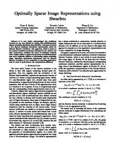
and the signals being analyzed have a sufficiently sparse representation. While it has been shown that there exist large overcomplete dictionaries that are very incoherent there is no guarantee that such a dictionary exists in which the signals of interest are sparse. Indeed the dictionary choice must be data driven to ensure that we are likely to be able to obtain a sparse representation. For audio, Gabor-like dictionaries (such as the MCLT used here) seem well-suited to this task, at least for the tonal components within the signal. Unfortunately the MCLT transform has a coherence µ ≈ 0.5. The most correlated atoms within the MCLT dictionary occur between neighboring frequency bins within the same synthesis frame, as illustrated in figure 1. This implies that here the 0.04

0.03

0.02

0.01

0

−0.01

−0.02

−0.03

−0.04 0

100

200

300

400

500 n

600

700

800

900

1000

Fig. 1. The real part of the k = 20 atom (solid) is plotted along side the imaginary part of the k = 21 atom (dotted) within the same analysis window. There is strong coherence between the neighboring atoms as these functions become in phase at the center of the frame.

OMP and BPDN approaches may well not find the maximally sparse solution. Instead we have chosen to use a fast converging algorithm desipite the fact that it is known to have potentially many local minima [5]. Experimentally 14

we have found that the local minima are always very good. For example, in the significance map coding in section 4.2.1, below, using BPDN resulted in a consistent 5dB reduction in SNR for a given number of significant coefficients over the range of different approximation levels considered. This appears to be predominantly due to an excessive shrinkage of the significant coefficients associated with l1 norm, since a similar performance to that in section 4.2.1 can be achieved by additional least squares post-processing on the significant coefficients (at a further increase in computation).

4

Numerical Experiments

To illustrate the FIRSP algorithm and the power of MCLT based overcomplete representations of audio we now present some numerical experiments. We begin by showing the speed with which the algorithm can generate a sparse solution to a real world (44.1kHz sampling rate) audio signal. We then explore the potential benefits that may be realized from using such a sparse representation in audio coding. Finally we show how the basic MCLT dictionary can be extended to a dual-resolution time-frequency representation while still being amenable to processing with the FIRSP algorithm.

4.1 A simple audio example

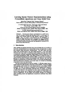
We first apply the algorithm to a short extract (approx. 6 seconds) from a guitar solo. The audio was sampled at 44.1kHz and we used an MCLT with a frame size of 1024. Figure 2 (left) shows the MCLT “spectrogram” for the audio signal. The signal was then processed using a fixed v = 10−5 and 10 iterates 15

of the FIRSP algorithm. In contrast to the initial redundant basis only 6% of the complex coefficients remained non-zero. The resulting approximation had a SNR of: 38dB. The generative MCLT “spectrogram” for the sparse coefficients is also shown in figure 2 (right). 4

4

x 10

2.2

2

2

1.8

1.8

1.6

1.6

1.4

1.4 Frequency (Hz)

Frequency (Hz)

2.2

1.2 1

1.2 1

0.8

0.8

0.6

0.6

0.4

0.4

0.2

0.2

0.5

1

1.5

2

2.5

3 3.5 Time (sec)

4

4.5

5

Iterate: 10

x 10

5.5

0.5

1

1.5

2

2.5

3 3.5 Time (sec)

4

4.5

5

5.5

Fig. 2. MCLT “spectrogram” of the guitar data (left) and the generative sparse MCLT approximation.

The evolution of the algorithm is best seen by plotting the size of the coefficients sorted in order of magnitude for each iterate, as in figure 3. Clearly most of the coefficients shrink to zero in a small number of iterates.

4.2 Coding Costs for the sparse MCLT

We next make a preliminary examination of the coding costs associated with a quantized sparse MCLT in comparison with the traditional quantized MDCT transform. We will concentrate on relatively simple coding structures and emphasize that we are not arguing that the following coding strategies are competitive with state-of-the-art audio coding. As with traditional transform coding, a high degree of sparsity in the quanitzed coefficients means that a substantial part of the coding cost can be taken up 16

0

10

−2

10

−4

10

−6

10

−8

10

−10

10

−12

10

−14

10

0

0.5

1

1.5

2

2.5

3 5

x 10

Fig. 3. A sorted plot of MCLT coefficient amplitude for each iteration of the FIRSP algorithm (solid lines - iterations increasing from right to left) and the magnitude of the basic MDCT coefficients are also shown (dashed).

coding the significance map (the map identifying which quantized coefficients are non-zero) [11]. We therefore consider the coding rate, R in two parts: R = Rsig map + Rcoef where Rsig map measures the total bit budget required to code the significance map and Rcoef measures the number of bits required to code the quantized non-zero coefficients. We begin by considering the cost of coding the significance map.

4.2.1 Coding the significance map If we treat the significance of each coefficient as independent, we can estimate the rate, Rsig map , as the sample entropy, Hsig map , of the significance map: R = Hsig map + Rcoef 17

where Hsig map = −(ps log ps + (1 − ps ) log(1 − ps )) and ps is the probability of a coefficient being non-zero. Note here we are dealing with the significance map of signal approximations. Exact representations would typically always have N significant coefficients. To measure Hsig map for the sparse MCLT approximation we used the same audio sample examined in the last section. Again the frame size was set to 1024 but this time 50 iterations of the FIRSP operator were applied to guarantee absolute convergence. We calculated the signal-to-noise ratio (SNR) for a range of sparse approximations using different v and plotted these against the coding cost for the significance map. For comparison we also included the SNRs for the best K−coefficient MDCT approximation for the signal over the same sparsity range. The graphs in figure 4 show that there is approximately a 5 dB gain in using the sparse MCLT approximation over the MDCT for a wide range of bit rates. Note that both the MDCT and the MCLT have the same size significance maps and are thus directly comparable. Further improvements in coding can be obtained by incorporating structure within the significance map into the coding strategy. Looking at figure 2 we see that the significance map exhibits strong persistence in time for each subband (other structure due to onsets and harmonicity is not considered here). The MDCT also exhibits this type of structure but to a lesser extent. A relatively simple way to code this structure is to use run length encoding along each subband followed by entropy coding. This has a dramatic effect on the coding cost, as shown in figure 4. Here it can be seen that both the MDCT and the sparse MCLT gain substantially from run-length encoding with a slightly bigger improvement (in percentage terms) for the MCLT ap18

Coding Cost vs. SNR 55

50

MDCT MDCT run−length encoded sparse MCLT sparse MCLT run−length encoded

45

40

SNR

35

30

25

20

15

10 −2 10

−1

10 Coding cost (bits per sample) for the significance map

0

10

Fig. 4. A plot of Signal-to-Noise Ratio against the significance map coding cost for: the MDCT with independent coding (solid); the sparse MCLT with independent coding (dashed); the MDCT with run-length encoding (dot-dashed); and the sparse MCLT with run-length encoding (dotted).

proximation.

4.3 Coding the non-zero coefficients

So far, of course, we have ignored the coding cost of the quantized non-zero coefficients values, Rcoef . As above, we consider a relatively simple coding strategy that treats each coefficient independently. We can then estimate the coding cost to be: R = Rsig map + ps Hcoef where Hcoef is the sample entropy of the non-zero quantized coefficients values (measured per significant coefficient). To do this we now need to introduce quantization schemes for the two methods. For the MDCT we have used a uniform quantizer with a double-sized zero bin [11]. To construct a similar quantizer for the complex MCLT coefficients we chose to use an Unconstrained 19

Polar Quantizer (UPQ) [21]. The coefficient amplitude is the same as the MDCT quantizer. The phase components is then uniformly quantized but with the number of phase quantization bins, nθ , being dependent on the amplitude value such that: nθ (k) = 6(k + 1/2) for the kth amplitude region (with the exception of the zero bin, k = 1, where there is no phase). This UPQ is designed to space the regions approximately uniformly to enable subsequent efficient use of entropy coding. When calculating the sample entropy of the MCLT, to avoid the problem of limited data, we calculated the sample entropy for the coefficient amplitudes only and then assigned a cost of log2 nθ (k) bits for the phase. For the MCLT we also need to select an appropriate quantization resolution for a given approximation level v. For this we use the following informal argument. The signal x is fully represented by the coefficients, u, and the residual, e. A possible coding strategy is to code both separately to the same resolution. However, while u is expected to be sparse and therefore provide good energy compaction, the residual, e is assumed Gaussian and is therefore a less efficient representation. A natural choice of quantization resolution is to select a level such that with high probability the residual term is coded as zero (thereby requiring zero bits). Interestingly this is the same requirement that has been proposed for threshold selection in signal de-noising [11] where it can be shown that setting T =

q

2v loge N should with high probability be just above the

level of the noise. We adopt this value here, setting the amplitude bin size to T . We also note that experimentally this does indeed appear to be close to optimal choice. The results for the total coding cost are presented in figure 5. While there is still a small amount of coding gain for the MCLT at very low bit rates (not 20

Reconstruction SNR vs. Total Coding Cost (bits per sample) 55

50

MDCT MDCT run−length encoded sparse MCLT sparse MCLT run−length encoded

45

40

SNR

35

30

25

20

15

10 −2 10

−1

0

10 10 Total Coding Cost (bits per sample)

1

10

Fig. 5. A plot of Signal-to-Noise Ratio against the total coding cost for: the MDCT (solid) and the sparse MCLT (dashed) with independent significance map coding; and the MDCT (dot-dashed) and the sparse MCLT (dotted) with run-length encoding for the significance map.

of general interest for practical audio, due to poor sound quality), in general the MCLT performs slightly worse than the MDCT. To see why this is we look in detail at the coding cost for SNR ≈ 27 dB (v = 10−4 ) where the rate-distortion performance is similar for both methods. The breakdown of the coefficient coding cost is displayed in table 1. From the table we can see that the cost of coding the amplitude in either case is virtually identical. It is therefore the additional phase cost that negates the sparsity coding gain for the MCLT. While our current results show no big coding gain for the sparse MCLT it still looks a competitive representation from these initial findings. Furthermore, for the MCLT, we should expect there to be more exploitable structure within the coefficient values themselves. For example when a subband is occupied by a single partial from a note, the temporal phase within that subband will be 21

Table 1 Coding Cost breakdown for non-zero coefficients (entropies in bits per significant coefficient). MDCT

MCLT

9353

5915

262144

262144

Amplitude Entropy

3.59

3.77

Sign/Phase Entropy

1.00

4.60

Coefficient Entropy

4.59

8.37

Total cost per sample, Rcoef

0.164

0.189

Number of non-zero coefficients Total number of coefficients

highly predictable (c.f. the phase vocoder). Similarly we might expect that the amplitude will vary smoothly in time along the note. It is more difficult to see how this structure could be exploited within the MDCT transform where, due to the lack of explicit phase information, there will be a complicated fluctuation in coefficient values within a subband. The MCLT structure also makes the inclusion of perceptually weighted cost functions substantially simpler.

4.4 A Dual-resolution time-frequency approximation

Sparse overcomplete time frequency representations also have a great potential in providing access to higher level information about the an audio signal, such as distinguishing between steady state tones and note onsets. This in turn can be extremely useful for signal processing applications such as audio modification, source separation, note detection/recognition, and automatic 22

music transcription. Here we show that the framework developed in this paper easily extends to allow an additive dual-resolution signal approximation. The MCLT dictionary can easily be extended to include multi-resolution representations, at the cost of a larger dictionary, by taking the union of multiple MCLT dictionaries with differing frame sizes. Here we consider two distinct resolutions: an MCLT with a frame size of 2048 samples (approximately 46 ms) and a frame size of 256 samples (approximately 6 ms). Since we still have a union of orthonormal bases we are able to apply the same fast iterative sparsification algorithm presented in section 3.2. Unfortunately a naive implementation of this can result in very slow convergence. One solution appears to be a judicious choice of initial condition. If we initialize the coefficients by sharing the signal energy equally between all 4 bases then convergence is painfully slow (several hundred iterates!). This is because the signal induces large coefficients in all bases. The transfer of energy is then achieved by small repeated shrinkage operations. We found that a better initialization was to begin with only the long frame MCLT representation and apply a couple of iterates of the shrinkage operator. The short frame MCLT bases were then included and used initially to model the residual of the long frame approximation. This has the effect of initializing the second set of coefficients to fit the signal that is most poorly represented by the sparse long frame MCLT (with a similar flavor to the hybrid coding scheme used in [2]). The resulting algorithm appeared to converge in 30-50 iterates. An alternative approach, proposed in [1], that is not explored here would be to initialize the coefficients with the Best Basis algorithm, the Matching Pursuit (see e.g. [10]) or any other (fast) approximate sparse representation. To demonstrate our dual-resolution approximation we applied the algorithm 23

to part of an MPEG standard test signal. This is a particularly good signal for our purposes since it contains strong ringing tones as well as sharp transients. Figure 6 shows plots of: the original signal, the tonal component (formed from the long frame MCLT), the transient component (formed from the short frame MCLT) and the residual. The approximation parameter, v, was set at 10−5 and the algorithm was run for 50 iterates. We can see that the addition of 0.2 0 −0.2 0.5

1

1.5

2

2.5

3

3.5

4

4.5

5

5.5

0.5

1

1.5

2

2.5

3

3.5

4

4.5

5

5.5

0.5

1

1.5

2

2.5

3

3.5

4

4.5

5

5.5

0.5

1

1.5

2

2.5

3

3.5

4

4.5

5

5.5

0.2 0 −0.2

0.2 0 −0.2

0.2 0 −0.2

Fig. 6. Time domain plots of: (a) the original signal; (b) the approximated transient component; (c) the approximated tonal component; and (d) the residual error

the short frame MCLT has allowed us to not only approximate the transients of the signal much better, but more importantly, it has provided us with a separation of the transient components which are localized in time but not frequency and steady state components which are localized in frequency but not time, as illustrated in figure 7. Thus this representation, although not perfect, simultaneously provides us with an excellent time and frequency localization of the transients and tones respectively (at least for music) 2 We now show 2

Note that this is a statement about inference and does not contradict Heisenberg’s

uncertainty principle since the finer resolution occurs in the generative (coefficient) domain. Each individual atom must, of course, still obey the uncertainty principle.

24

Fig. 7. The significance map for the transient components (top left); the significance map for the tonal components (top right); the combined significance map (bottom left);and, for comparison, the spectrogram for the original signal (bottom right).

how the decomposition can subsequently be used for audio modification.

4.4.1 Note extraction A difficult task in such an audio signal is the extraction of a single note. If we were using a fixed resolution time frequency approximation (irrespective of sparsity) then without additional high level information the extraction of a single note would have to be done using some form of time-frequency mask. However this will introduce distortions whenever notes overlap in the time frequency domain. For our signal this would be most acute where the tones 25

intersect with the transients. In contrast, because we have a fully additive representation that maps the transient and the tonal components to different spaces, we can extract notes even where transient and tonal components intersect. To demonstrate this we manually grouped TF elements from both the transient and steady state dictionaries associated with the 7th note in the signal. To extract the note we simply zero these coefficients (applying two masks separately to the short and long frame coefficients. Figure 8 shows plots of (a) the signal with the note removed and (b) the note itself. The resulting audio sounded as though the note had never been present. That we have not com0.2 0.1 0 −0.1 −0.2 0.5

1

1.5

2

2.5

3

3.5

4

4.5

5

5.5

0.5

1

1.5

2

2.5

3

3.5

4

4.5

5

5.5

0.5

1

1.5

2

2.5

3

3.5

4

4.5

5

5.5

0.2 0.1 0 −0.1 −0.2

0.2 0.1 0 −0.1 −0.2

Fig. 8. Time domain plots of: (a) the sparse reconstruction (b) the reconstruction with the 7th note removed ; and (c) the removed note.

promised overlapping notes can be seen in figure 9 where the spectrograms of the sparse approximation with and without the seventh note are shown. There is clearly huge potential for extending this to more complex modifications. For example we could easily move the note position (to possibly correct a mis-timed note) or alter its sound before replacing it. 26

4

4

x 10

2

2

1.5

1.5

Frequency

Frequency

x 10

1

0.5

0

1

0.5

0

1

2

3 Time

4

0

5

0

1

2

3 Time

4

5

Fig. 9. The spectrograms for: the sparse approximation (top); and the the same signal with the seventh note removed (bottom).

5

Conclusions

In this paper we have introduced an efficient means of generating a sparse approximation for audio signals in the form of an overcomplete subband representation. The method is sufficiently fast to enable the processing of full CD quality (44,100 samples per second) audio data, without downsampling. We further examined the potential of this representation as the basis of a sparse coding strategy. The high degree of sparsity means that there are substantial savings in encoding the significance map for the signal. However the full coding cost is a function of both the significance map and the cost of coding the values of the significant coefficients. While we have made some preliminary observations in this direction, to make a full and fair comparison with state-of-the-art audio coders we would need to develop a complete coding scheme, which is beyond the scope of this paper. The approach advocated here tentatively provides a structure that lies in-between traditional transform/subband coding, such as MP3, and low rate parametric codes, such as the MPEG HILN coder, with the possibility of gaining benefits from both 27

approaches. Finally we have shown that the generalized IRLS framework is very flexible and, in particular, can be extended to include multi-resolution time-frequency approximations. These could be used to further improve the coding of audio signals or, as demonstrated here, be used in signal separation and modification applications. Our current research is focusing on a number of open questions and problems that have arisen from this work and we end by mentioning a number of these that we feel are of particular interest to the field. How overcomplete should a dictionary be? Currently in the work on overcomplete representations there has been little said about how overcomplete the dictionary should be (2×? 10×? 100×? ...). What are good measures of quality for a dictionary? A fair amount of attention has been paid to the incoherence of a dictionary and how it effects the complexity of determining sparse representations. However we believe that there is a need for a finer tool to determine the performance of a given dictionary. In particular, such a measure should also probably be signal dependent (see for example [17]). Extensions to other signal types. We have recently also considered the use of generalized IRLS algorithms to images [5]. Here, the equivalent dictionary to the MCLT is Kingsbury’s Dual Tree Complex Wavelet Transform, however other dictionaries might prove more appropriate. Extensions to structured priors. We saw in section 4.2.1, that even more parimonious representations can be obtained by exploiting the structure of the significance map. So far this structure has been treated separately to 28

the generation of the sparse approximation. However it would be interesting to develop algorithms that simultaneously generated structured and sparse approximations.

Acknowledgements

The authors would like to thank the Centre for Digital Music at Queen Mary for many useful discussions and Pierre Vandegheynst for making us aware of a number of useful references. LD would also like to acknowledge the support of the French Ministry of Research and Technology, under contract ACI “Jeunes Chercheuses et Jeunes Chercheurs” number JC 9034.”

References

[1] S. Chen and D.L. Donoho, ”Atomic decompostion by basis pursuit”, SIAM J. Sci. Computation, Vol. 20, No 1, pp 33-61, 1999. [2] L. Daudet and B. Torr´esani, “Hybrid representations for audiophonic signal encoding,” Signal Processing, vol. 82, No. 11, pp. 1595-1617, 2002. [3] M. E. Davies and L. Daudet, “Sparsifying Subband Decompositions” Proc. of IEEE Workshop on Appl. of Sig. Proc. to Audio and Acoustics, Oct. 2003. [4] M. E. Davies and L. Daudet, “Fast sparse subband decomposition using FIRSP”, Proc. EUSIPCO 04, 2004. [5] M. E. Davies, T. Blumensath and L. Daudet, “Generalized IRLS schemes for sparse signal approximation”, in preparation, 2004.

29

[6] A. P. Dempster, N. M. Laird and D. B. Rubin, ”Maximum likelihood from incomplete data via the EM algorithm”, J. Roy. Statistical Soc. Ser. B, Vol. 39, no 1, pp1-38,1977. [7] M. Figueiredo, ”Adaptive sparseness using Jeffreys prior” Neural Information Processing Systems (NIPS), MIT Press, 2001. [8] I. F. Gorodnitsky and B. D. Rao, “Sparse signal reconstruction from limited data using FOCUSS: a re-weighted minimum norm algorithm,” IEEE Trans. SP, vol 45(3), 1997. [9] M.S. Lewicki and T.J. Sejnowski, “Learning overcomplete representations,” Neural Computation, vol. 12, pp. 337-365 2000. [10] S. Mallat and Z.Zhang, ”Matching pursuit with time-frequency dictionaries”, IEEE Trans. Signal Processing, vol. 41 pp 3397-3415, 1993. [11] S. Mallat, ”A wavelet tour of signal processing”, Academic Press, 1999. [12] H. Malvar, ”A modulated complex lapped transform and its applications to audio processing”, ICASSP’99, 1999. [13] G.J. McLachlin and T. Krishnan, The EM Algorithm and Extensions, Wiley Series in Probability and Statistics, 1997. [14] B.D. Rao, K. Engan, S.F. Cotter, J. Palmer and K. Kreutz-Delgado, “Subset Selection in Noise Based on Diversity Measure Minimization,” IEEE Trans. SP, vol. 51(3), pp.760-770, 2003. [15] S. Sardy. A. G. Bruce and P. Tseng, “Block coordinate relaxation methods for nonparametric wavelet denoising,” Comp. and Graph. Stat., vol. 9(2), 2000. [16] M.E. Tipping, “Sparse Bayesian Learning and the Relevance Vector Machine,” J. of Machine Learning, vol. 1 pp. 211-244, 2001.

30

[17] S. Molla and B. Torr´esani, “Determining local transientness in audio signals”, IEEE Signal Processing Letters, vol. 11 No. 7, pp. 625-628, 2004. [18] J. A. Tropp, “Greed is Good: algorithmic results for sparse approximation” IEEE Trans. IT ol. 50(10), pp. 2231-2242, 2004. [19] J. A. Tropp, “Just Relax: convex programming methods for subset selection and sparse approximation”, ICES report 04-04, 2004. [20] M. West, ”On scale mixtures on normal distributions”, Biometrika, Vol 74 No. 3, pp 646-648, 1987. [21] S. G. Wilson, “Magnitude/phase quantization of independent Gaussian variates”, IEEE Trans. Communications, vol. 28, pp1924-1929, 1980. [22] R.W.Young and N.Kingsbury, ”Frequency domain motion estimation using a complex lapped transform”, IEEE Trans. Image Processing vol. 2 pp 2-17, 1993. [23] M. Zibulevsky and B. A. Pearlmutter, “Blind separation of sources with sparse representations in a given signal dictionary,” Neural Computation, vol. 13(4) pp. 863-882, 2001.

31