SPARSE REPRESENTATION AND LEAST SQUARES-BASED CLASSIFICATION. IN FACE RECOGNITION. Michael Iliadisâ, Leonidas Spinoulasâ, Albert S.
SPARSE REPRESENTATION AND LEAST SQUARES-BASED CLASSIFICATION IN FACE RECOGNITION Michael Iliadis? , Leonidas Spinoulas? , Albert S. Berahas† , Haohong Wang‡ , Aggelos K. Katsaggelos? ? †
Dept. of Electrical Engineering and Comp. Sc., Northwestern University, Evanston, IL 60208, USA Dept. of Eng. Sciences and Appl. Mathematics, Northwestern University, Evanston, IL 60208, USA ‡ TCL Research America, San Jose, CA 95134, USA ABSTRACT
In this paper we present a novel approach to face recognition. We propose an adaptation and extension to the state-of-the-art methods in face recognition, such as sparse representation-based classification and its extensions. Effectively, our method combines the sparsity-based approaches with additional least-squares steps and exhitbits robustness to outliers achieving significant performance improvement with little additional cost. This approach also mitigates the need for a large number of training images since it proves robust to varying number of training samples. Index Terms— Face recognition, sparse representation, classification. 1. INTRODUCTION One of the most popular problems in computer vision is face recognition (FR) which focuses on deducing a subject’s identity through a provided image [1]. Over the last decade, researchers have been focusing on addressing practical largescale FR systems in uncontrolled environments [2]. Recently, face recognition via sparse representation-based classification (SRC) [3] and its extensions [4, 5] have proven to provide state-of-the-art performance. The main idea is that a subject’s face sample can be represented as a sparse linear combination of available images of the same subject captured under different conditions (e.g., poses, lighting conditions, etc.). The same principle can also be applied when a face image itself is represented in a lower dimensional space describing important and easily identifiable features. In order to enforce sparsity, `1 optimization algorithms [6, 7] can be employed. Then, the face class that yields the minimum reconstruction error is selected in order to classify or identify the subject, whose test image or sample is available. Sparse coding has also been proposed to jointly address the problems of blurred face recognition and blind image recovery [8]. Furthermore, it has been utilized in [9] to deduce a transformation-invariant face recognition algorithm as well as in [10] to extend the SRC framework for handling misalignment, pose and illumination invariance.
526
Despite their success, the necessity of `1 optimization methods for improved face recognition rates has been recently criticized [11, 12]. Zhang et. al. argued that FR performance improvement stems from the collaborative representation of one image using multiple similar images rather than the usage of the `1 norm in the optimization procedure, and proposed a simpler regularized least squares formulation to solve the FR problem. Furthermore, the authors in [11, 13] state that `1 norm techniques can only be successful under certain conditions. Specifically, Wright et. al. state in [13]: “The sparse representation based face recognition assumes that the training images have been carefully controlled and that the number of samples per class is sufficiently large. Outside these operating conditions, it should not be expected to perform well.” In order to overcome the limitation of requiring large amounts of samples per class, Deng et. al. [4, 5] proposed the use of additional dictionaries, constructed using the available data, to refine FR performance. The motivation for this work comes from the fact that different images of the same subject share a lot of similarities; hence, an additional intra-class generic dictionary of subject samples could effectively model face variations. In this method, which is called Extended SRC (ESRC), the test sample is represented as a sparse linear combination of the training and intra-class dictionary samples. In this work, we show that sparsity-based approaches can be effectively combined with additional least-squares steps to provide significant performance improvement with little additional cost. Moreover, the proposed approach can overcome the need for a large number of training images since it proves robust to varying number of training samples as we will show in the experimental section. This paper is organized as follows. Section 2 overviews existing face recognition classifiers and presents their modeling. The proposed face recognition algorithm is analyzed in Section 3. Finally, experimental results and discussion about the performance of the proposed approach are presented in Section 4 and conclusions are drawn in Section 5.
Algorithm 1 The SRC Algorithm
2. RELATED WORK In this section we survey face recognition algorithms based on sparse representation and regularized least squares. Let y ∈ Rd denote the face test sample, where d is the dimensionality of a selected face feature and T = [Ti , . . . , Tc ] ∈ Rd×n denote the matrix (dictionary) with the set of samples of c i subjects stacked in columns. Ti ∈ Rd×n P denotes the ni set th of samples of the i subject, such that, i ni = n. Sparse Representation-based Classification (SRC) [3]: In SRC, the test sample y is represented by, y = Ta + e, d
(1) n
where e ∈ R is dense noise and a ∈ R is a sparse vector with nonzero elements corresponding to few samples in T. Thus, the test sample can be represented as a sparse linear combination of the samples in T. The coefficients of a can be estimated solving the optimization problem, ˆ = argmin ky − Tak22 + λ kak1 . a
(2)
a
The complete steps of the SRC algorithm are presented in Algorithm 1. Extended SRC (ESRC) [4]: In ESRC, the test sample y is represented by, y = Ta + Vb + e, (3) where V ∈ Rd×n is a variation dictionary that models intraclass variant bases, such as, lighting changes, exaggerated expressions, or occlusions, for the representation of each subject i, while a ∈ Rn is a sparse vector, as in SRC. Different types of variations, that cannot be captured by V, are represented by the dense noise term e ∈ Rd . Vector b ∈ Rn is also considered to be sparse and its coefficients can effectively capture the contribution of uncontrolled viewing conditions in the final image and are, hence, not informative about the subject’s identity. Thus, the test sample is represented as the linear combination of Ta, capturing the subject’s identity, and Vb, capturing sparse noise terms. The variation matrix V can be constructed by the differences of each sample to its corresponding’s class centroids, as suggested in [4], V = [T1 − m1 rT1 , . . . , Tc − mc rTc ], where mi = T
1 ni Ti ri ni
(4)
is the centroid of class i, and ri =
[1, . . . , 1] ∈ R . In ESRC, the sparse vectors a and b can be obtained by,
� � � 2 �
a a ˆ
. (5) ˆ, b = argmin y − [T, V] a − λ b 2 b 1 a,b Similar to SRC, classification (or else subject identification) is performed by selecting the class i that provides the smallest residual. The difference is that in computing the residual
527
Inputs: Vector y and matrix T. 1. Normalize the columns of T to have unit `2 -norm. ˆ solving the problem in (2). 2. Estimate the sparse vector a 3. Compute the residuals for each class i as, ˆi k2 , ei (y) = ky − Ti a ˆi is the segment of a associated with class i. where a Output: Identity of y as, Identity(y) = argmini {ei }
of each class, the term Vb is also subtracted from the test sample. Regularized least squares (CR-RLS) [12]: In CR-RLS a regularized least squares method is proposed in order to collaboratively represent the test sample without imposing sparsity constraints on the unknown variable a. Again, classification is performed by minimizing the reconstruction term for each class. The optimization problem, of this very efficient method, is given by, ˆ = argmin ky − Tak22 + λkak22 , a
(6)
a
which can be easily solved in closed form. 3. SPARSE REPRESENTATION AND REGULARIZED LEAST SQUARES Let the linear representation of the test sample, y, be given by (3). In [4], a and b were regularized using the `1 norm. As Zhang et. al. showed in [12], when increasingly many training samples are used for the representation of a test sample, the discriminating ability between classes reduces, leading to comparably small reconstruction errors for all classes. Thus, sparsity of coefficients should be considered so that only a few training samples represent the test sample. Similarly, if there are redundant and overcomplete facial variant bases in V, the combination coefficients in b are naturally sparse. In the proposed Sparse Representation and Regularized ˆ Least Squares (SR+RLS) method, an initial estimation of a ˆ is obtained by solving the ESRC problem in (5). Ideand b ally, this initial estimation will provide us with the largest coefficients at locations of vector a corresponding to the class that the test sample belongs to. In other words, we expect this class to exhibit the smallest residual compared to other classes. However, due to face variations this may not always be the case, and the coefficient values in a could be noisy. ˆ through the optimization problem in (5), Having estimated a we expect that the test sample is best represented as a linear combination of training samples of its true class. Nevertheless, the corresponding mixing coefficients need not be the largest.
The decision of the correct identity in SRC is dictated by the minimum residual. In this work we account for the possibility of the correct identity hiding under slightly higher residuals than the minimum, due to face variations. Thus, we propose a novel face recognition algorithm that is solved in four separate steps. ˆ solving the optimization probˆ and b 1. We first estimate a lem in (5). ˆ, we construct a new 2. Based on the initial estimation of a face dictionary that consists of the training samples of ˆ are the classes whose corresponding coefficients in a nonzero, while the remaining sets of training samples for all other classes are nullified (set to zero). 3. Having constructed the new smaller dictionary we can estimate the new coefficients by solving a regularized least squares problem. 4. Finally, the face identity will be chosen based on the minimum class residual provided by the updated coefficients. Next, we discuss the aforementioned steps in more detail. 3.1. The Sparse Representation (SR) step ˆ we solve ˆ and b In order to obtain the initial estimation of a the problem in (5). This is a standard sparse coding problem and can be solved using any `1 minimization algorithm, such as Homotopy [14]. 3.2. Dictionary construction ˆi is the segment of a ˆ associLet the function f (ˆ ai ), where a ated with class i, be given as, ( ˆi = 0 0, if a f (ˆ ai ) = . (7) 1, otherwise ˜ is constructed as follows, Then the new dictionary T ˜ = [f (ˆ T ai ) Ti , . . . , f (ˆ ac ) Tc ] ∈ Rd×n
(8)
Algorithm 2 Classification based on SR+RLS Algorithm Inputs: Vector y and matrix T. 1. Construct the variation matrix V using (4). 2. Apply PCA on the training samples T and project T and V onto a d dimensional space. 3. Normalize the columns of T and V to have unit `2 norm. ˆ solving the problem in (5). ˆ and b 4. Estimate a ˜ using the estimated coefficients 5. Construct dictionary T ˆ and estimate ˆf using the problem in (9). in a 6. Compute the residuals for each class i as,
ei (y) = y − Ti ˆfi , 2
where ˆfi is the coding coefficient vector associated with class i. Output: Identity of y as, Identity(y) = argmini {ei } .
The solution to problem (9) has the following properties, • The RLS step is more likely to provide the true identity since we reconstruct for fewer classes and thus less noise. • We expect ˆf to have larger coefficient values corresponding to the true identity’s training samples compared to the ˆ through (5). initial estimate a ˜ is expected to • The problem in (9) is well-defined since T consist of fewer (nonzero) columns than rows. Thus, RLS is appropriate for solving such problem. • We do not add significant complexity to the solution since the least squares step in (10) can be solved very efficiently. 3.4. The SR+RLS classification The SR+RLS algorithm is summarized in Algorithm 2. An example of our method is presented in Figure 2.
where denotes the convolution operator.
4. EXPERIMENTAL RESULTS
3.3. The Regularized Least Squares (RLS) step Having constructed the new dictionary with most training samples suppressed to zero, we can obtain a new estimation vector by solving the regularized least squares problem,
2 2 ˆf = argmin ˜
y − Tf
+ λkf k2 . f
2
(9)
The problem in (9) has the closed form solution, � �−1 ˆf = T ˜TT ˜ + λI ˜ T y, T
(10)
where ˆf ∈ Rn is the vector with nonzero coefficients only at locations where the training samples are not zero, and λ > 0 is a constant.
528
In this section we present experiments on publicly available databases, AR [15] and Extended Yale B [16], to show the efficacy of the proposed method. In order to solve the `1 minimization problem we use the Homotopy method [14]. We compare our method with SRC [3], ESRC [4] and CRRLS1 [12]. For SRC and ESRC we set the regularization parameter λ = 0.005 as proposed in [4] and for CR-LRS we set λ = 0.001 as suggested in [12]. For fair comparisons, we set the same parameters in our algorithm as the other methods: λ = 0.005 for the `1 problem and λ = 0.001 for the regularized least squares problem. All parameters remain the same for both databases. As input facial features we use Eigenfaces with d = 300. 1 Source
code obtained from author’s website.
0.25
0.25
Table 1: Recognition rate on the AR database.
0.2 0.2 0.15
Algorithms SRC [3] ESRC [4] CR-RLS [12] SR+RLS
0.1 0.15 0.05
0 0.1 −0.05
−0.1 0.05 −0.15
0
−0.2 0
200
400
600
800
1000
0.9
1200
1400
0
200
400
600
800
1000
1200
Recognition rate 92.49 ±0.82 96.98 ±0.46 96.80 ±0.54 98.07 ±0.38
Time 0.0266s 0.0982 0.0002s 0.1040s
1400
1.1
1.05
Table 2: Recognition rate on the Extended Yale B database.
0.85 1
Algorithms SRC [3] ESRC [4] CR-RLS [12] SR+RLS
0.95 0.8
0.9
0.75 0.85
0.8 0.7 0.75
0.65
Recognition rate 97.17 ±0.62 96.65 ±0.76 97.78 ±0.49 98.11 ±0.23
Time 0.0339s 0.0630s 0.0002s 0.0747s
0.7 0
10
20
30
40
50
60
70
80
90
100
0
10
20
30
40
50
60
70
80
90
100
Fig. 1: The top left figure shows an example face, belonging to identity 4, occluded with a scarf. The upper left plot shows the coeffiˆ using the problem in (5). The upper cient values of the estimated a right plot shows the coefficient values of ˆf estimated by the problem in (9). The lower two plots show the estimated residuals after solving problems (5) and (9) from left to right, respectively. ESRC would classify this face as identity 29 since the lowest residual is at index 29 while the re-estimation of coefficients, as described in Section 3.3, results in the correct classification of the image providing the minimum residual at index 4.
Fig. 2: Example images from the AR database. This database is more challenging than the Yale, since more subjects need to be recognized while there exhibits large face variations within each class.
4.1. AR database This experiment is a reproduction of that in section 5 of [11]2 . The AR database consists of over 3000 frontal images of 126 individuals. There are 26 images of each individual, and each person participated in two sessions, separated by two weeks. The faces in AR contain variations such as changes in illumination, expressions and facial disguises (e.g., sunglasses or scarfs). Example images of this database are shown in Figure 2. In our experiments, 100 subjects were randomly chosen (50 male and 50 female). For each subject, we randomly permute the 26 images, and then take the first half for training and the rest for testing. Thus, we have 1300 training and 1300 testing samples. For statistical stability, we generate 10 different training and testing dataset pairs by randomly per2 The method in [11] is very similar to the CR-LRS [12]. The difference is that in [12] a regularization `2 norm term is incorporated. However, with λ = 0.001 set to a relative small number the results were the same
529
muting 10 times. The images are cropped to have dimensions 165 × 120 pixels and converted to gray-scale. Table 1 shows the recognition rates for this experiment. SR+RLS achieves the highest performance with 98.07% while ESRC has the second best recognition rate, slightly better than CR-RLS. 4.2. Extended Yale B database The extended Yale B dataset consists of 2414 frontal face images of 38 subjects. They are captured under various lighting conditions. They are cropped to have dimensions 192 × 168 pixels and normalized. For each subject, we randomly select half of the images for training (i.e., about 32 images per subject) and the other half for testing. Again for each subject, we randomly permute the images per subject and take the first half for training and the rest for testing. For statistical stability, we generate 10 different training and testing dataset pairs. In Table 2 we report the performance for this experiment. Again, SR+RLS achieves the highest recognition rate with 98.11%. CR-RLS achieves the second best, while ESRC has even lower performance than SRC. 4.3. Recognition from fewer training samples In order to show the robustness of our proposed method we evaluate AR and Extended Yale B databases with fewer training samples per subject keeping the same number of test samples. For the AR database, we perform two experiments, where we randomly choose 8 (AR 8) and 4 (AR 4) training samples per subject. In the Yale database we randomly choose 8 training samples per subject. Again, for statistical stability, we generate 10 different training and test dataset pairs. The results are presented in Table 3. It is apparent that, with fewer training samples, SRC’s performance reduces dramatically, which is consistent with the observations in [11, 12]. On the other hand, our method proves its robustness even with fewer training samples per subject outperforming the state-of-the-art methods.
Table 3: Recognition rate on the AR and Extended Yale B databases using reduced training samples. Algorithms SRC [3] ESRC [4] CR-RLS [12] SR+RLS
Yale 8 85.15 ±1.02 84.49 ±1.29 88.51 ±1.06 88.87 ±0.65
AR 8 84.52 ±0.79 93.30 ±1.23 93.99 ±0.64 95.48 ±0.58
AR 4 69.12 ±1.58 83.73 ±0.91 85.06 ±0.90 85.12 ±1.04
[4] W. Deng, J. Hu, and J. Guo, “Extended SRC: Undersampled face recognition via intraclass variant dictionary,” IEEE Trans. Pattern Anal. Mach. Intell., vol. 34, no. 9, pp. 1864–1870, Sept. 2012. [5] W. Deng, J. Hu, and J. Guo, “In defense of sparsity based face recognition,” in IEEE Conf. Comp. Vision Pattern Recognition, Jun. 2013, pp. 399–406.
4.4. Discussion The following conclusions are drawn based on the results on the two tested databases: 1. For both databases, SR+RLS outperforms SRC, ESRC and CR-RLS either with all training samples or few training samples. 2. ESRC has lower recognition rate for the Yale B database than the SRC when multiple training samples are considered. Instead, SR+RLS is consistent in performance in both databases for all cases. 3. Our method has the lowest time performance compared to the other methods. However, the overhead of the regularized least squares step is insignificant compared to the initial `1 estimation. All experiments were conducted in MATLAB on a 3.0 GHz PC with 8 GB RAM. 5. CONCLUSIONS
[6] E. J. Cand`es, J. Romberg, and T. Tao, “Robust uncertainty principles: Exact signal reconstruction from highly incomplete frequency information,” IEEE Trans. Inf. Theory, vol. 52, no. 2, pp. 489– 509, 2006. [7] Y. Tsaig and D. L. Donoho, “Compressed sensing,” IEEE Trans. Inf. Theory, vol. 52, pp. 1289–1306, 2006. [8] H. Zhang, J. Yang, Y. Zhang, N. M. Nasrabadi, and T. S. Huang, “Close the loop: Joint blind image restoration and recognition with sparse representation prior,” in IEEE Int. Conf. Comp. Vision, Nov. 2011, pp. 770–777. [9] J. Huang, X. Huang, and D. Metaxas, “Simultaneous image transformation and sparse representation recovery,” in IEEE Conf. Comp. Vision Pattern Recognition, Jun. 2008, pp. 1–8. [10] A. Wagner, J. Wright, A. Ganesh, Z. Zhou, H. Mobahi, and Y. Ma, “Toward a practical face recognition system: Robust alignment and illumination by sparse representation,” IEEE Trans. Pattern Anal. Mach. Intell., vol. 34, no. 2, pp. 372–386, Feb. 2012.
In this work, we presented a novel approach to face recognition effectively combining sparse representation and regularized least squares-based classification. We show that a simple additional least squares step in the optimization procedure can provide noticeable performance improvement while being robust to varying numbers of training samples in the dictionary. Hence, we manage to improve the face recognition performance of l1 minimization schemes even with low availability of training data samples, despite the criticism that such methods are not beneficial under lack of numerous samples per class.
[11] Q. Shi, A. Eriksson, A. Van den Hengel, and C. Shen, “Is face recognition really a compressive sensing problem?,” IEEE Conf. Comp. Vision Pattern Recognition, vol. 0, pp. 553–560, 2011.
REFERENCES
[14] D. L. Donoho and Y. Tsaig, “Fast solution of l1norm minimization problems when the solution may be sparse.,” IEEE Trans. Inf. Theory, vol. 54, no. 11, pp. 4789–4812, 2008.
[1] W. Zhao, R. Chellappa, P. J. Phillips, and A. Rosenfeld, “Face recognition: A literature survey,” ACM Comput. Surv., vol. 35, no. 4, pp. 399–458, Dec. 2003. [2] E. G. Ortiz and B. C. Becker, “Face recognition for web-scale datasets,” Comput. Vis. Image Underst., vol. 118, pp. 153–170, Jan. 2014. [3] J. Wright, A. Y. Yang, A. Ganesh, S. S. Sastry, and Yi Ma, “Robust face recognition via sparse representation,” IEEE Trans. Pattern Anal. Mach. Intell., vol. 31, no. 2, pp. 210–227, Feb. 2009.
530
[12] D. Zhang, M. Yang, and X. Feng, “Sparse representation or collaborative representation: Which helps face recognition?,” in IEEE Int. Conf. Comp. Vision, Nov. 2011, pp. 471–478. [13] J. Wright, Y. Ma, J. Mairal, G. Sapiro, T. S. Huang, and S. Yan, “Sparse representation for computer vision and pattern recognition,” Proc. IEEE, vol. 98, no. 6, pp. 1031–1044, Jun. 2010.
[15] Aleix Mart´ınez and Robert Benavente, “The AR face database,” Tech. Rep. 24, Computer Vision Center, Bellatera, Jun. 1998. [16] A. S. Georghiades, P. N. Belhumeur, and D. Kriegman, “From few to many: Illumination cone models for face recognition under variable lighting and pose,” IEEE Trans. Pattern Anal. Mach. Intell., vol. 23, no. 6, pp. 643–660, Jun. 2001.