Spatial mapping of growing degree days: an ... - University of Calgary

Journal of Applied Remote Sensing, Vol. 1, 013511 (24 April 2007)

Spatial mapping of growing degree days: an application of MODIS-based surface temperatures and enhanced vegetation index Quazi K. Hassan,a Charles P.-A. Bourque,a Fan-Rui Meng,a and William Richardsb a

Faculty of Forestry & Environmental Management, University of New Brunswick, Fredericton, New Brunswick, Canada, E3B 6C2 [email protected] b Environment Canada, Adaptation and Impacts Research Division, c/o University of New Brunswick, Fredericton, New Brunswick, Canada, E3B 6C2 Abstract. Growing degree days (GDD) is a simple temperature-based index of biological development. In this paper we evaluated the potential of using 2003-2005 MODIS-based 8day and 16-day composites of daytime surface temperature (TS) and enhanced vegetation index (EVI) values at 250 m resolution for mapping GDD. The work was applied to the Canadian Atlantic Maritime Ecozone as a demonstration of the methodology. The work proceeded by establishing an empirical relationship between mean tower-based estimates of TS for the MODIS-acquisition period of 10:30 am-12:00 pm and the daily mean TS calculated from half-hourly emitted infrared/longwave radiation measurements taken from four flux sites in southern commercial forests of Canada. The relationship revealed a strong correlation between variables (r2=98.4%) and was central to the calculation of daily mean TS from MODIS-based estimates of TS. Since seasonally-based estimates of GDD and EVI were strongly correlated (r2=87%), data fusion techniques were applied to enhance the GDD map originally produced at 1 km resolution (from infrared emission band data), to 250 m. In general, the MODIS-derived map of GDD showed a positive constant offset of about 511 degree days from calculated long-term averages (1971-2000) based on temperatures collected at 101 Environment Canada climate stations. Keywords: data fusion, enhanced vegetation index, growing degree days, MODIS, surface temperature.

1 INTRODUCTION Temperature and growing degree days (GDD) represent two important spatially-dynamic climatic variables, as both play vital roles in influencing forest development [1] by directly affecting plant functions such as evapotranspiration, photosynthesis, plant respiration, and inplant water and nutrient movement. Understanding the spatial distribution of GDD is crucial to the practice of sustainable forest management and agriculture, as GDD relates to the integration of growth. The focus of this paper is to develop a practical methodology to spatially estimate seasonal values of GDD using MODIS-based measurements of surface temperature and index-values of vegetation greenness applied over a forest-dominated portion of the Canadian Atlantic Maritime Ecozone. The most widely practiced and standard protocol for estimating GDD (typically, given as a unitless quantity) is to use daily mean air temperature acquired at approximately 1.5-2 m above grassed surfaces,

, GDD = T − T a base

© 2007 Society of Photo-Optical Instrumentation Engineers [DOI: 10.1117/1.2740040] Received 8 Jan 2007; accepted 21 Apr 2007; published 24 Apr 2007 [CCC: 19313195/2007/$25.00] Journal of Applied Remote Sensing, Vol. 1, 013511 (2007)

(1)

Page 1

(Ref. 2), T is the daily mean air temperature (in oC) derived from the measurements of daily a maximum and minimum air temperatures, and Tbase is the base temperature (in oC) below which vegetation ceases to be biologically active. When calculated from climate station data, GDD provides precise point estimates. For greater spatial representation, normally interpolative (gridding) methods, like kriging, inverse distance weighing, and natural neighbour, among others, are used to generate continuous surfaces [3]. Different gridding methods produce significantly different surfaces for the same input data and, as a result, quality of the interpolation is very much a function of the method employed. Also, because these methods rely on uncovering patterns inherent in the data, independent (explanatory) variables like elevation, terrain configuration, and other underlying variables that may perhaps cause variation in the data field cannot be directly used in interpolation. Usually increasing the number of data points will help address this variation, if gradual enough. Augmenting existing data networks is sometimes not feasible due to the cost involved, initial purpose of the network, and infrastructural problems in remote areas. Remote sensing platforms can, however, provide a solution to this by providing nearly continuous spatial coverage. Remote sensing techniques were used in the past to calculate GDD. The most common approaches used optical remote sensing to derive normalized difference vegetation index (NDVI: a measure of vegetation greenness) to provide long-term expressions of GDD; for some example approaches, refer to Table 1. Table 1. Examples of estimating GDD using optical RS data

Approach*

Source Ref. 4

•

Used a portable radiometer to generate growing-season, 10-day composite of NDVI for 1995 over tall grass prairie ecosystems (C3/C4) in Kansas, USA in monitoring ecological disturbance. • Demonstrated that the transformation using normalized integrated NDVI with GDD is a significantly better discriminator (p=0.0102). Ref. 2 • Used AVHRR-derived monthly composites of NDVI for the years 1983 through to 1992 over China for determining eco-climatic parameters, including, GDD and rainfall. • Air temperatures from 160 climate stations were used to generate GDD; and 155 out of 160 stations showed that the NDVI-to-GDD correlation was significant at the 0.05 level. Ref. 5,6 • Used AVHRR-derived time series (1985-1988 and 1995-1999) of NDVI over Kazakhstan for analyzing agricultural land cover change, and northern high-latitude region studied as part of the IGBP for analysis of land surface vegetation phenology. • Determined NDVI as a quadratic function of GDD in the quantification of land surface vegetation phenology changes. Ref. 7 • Used 15-day composites of GIMMS-NDVI for the period 1982 through 2002 in Fennoscandia in characterizing birch phenology. • Data from 20 meteorological stations were used to produce GDD time-series. Correlation coefficients between GDD and TI NDVI, ranged between 77%-99%, with a mean value of 91%. * Note: AVHRR-Advanced Very High Resolution Radiometer; GDD-growing degree day; GIMMSGlobal Inventory Monitoring and Modelling Studies; IGBP-International Geoshpere-Biosphere Program; NDVI-normalized difference vegetation index; TI NDVI-time integrated normalized difference vegetation index.

Since vegetation greenness depends on GDD accumulation, in theory, GDD should be strongly correlated to NDVI. However, NDVI has a tendency to saturate over dense vegetation, such as over dense deciduous forests at the height of the growing season [8, 9].

Journal of Applied Remote Sensing, Vol. 1, 013511 (2007)

Page 2

Instead of using the GDD-NDVI approach, we propose to use MODIS-based surface temperature (TS) for the initial calculation of GDD at 1 km spatial resolution by means of Eq. (1); here we assume that the daily mean air temperature is approximated by the daily mean surface temperature (a function of emitted infrared/longwave radiation). In order to enhance the spatial resolution of GDD to 250 m, we opted to use data fusion techniques to augment the 1 km resolution map to 250 m using the seasonally-averaged MODIS-derived enhanced vegetation index (EVI: Ref. 10) as a predictor (“in-filling”) variable of GDD. EVI is suitable replacement to NDVI, because EVI exhibits sensitivity across forest densities [8, 9] and has an effective resolution smaller than the 1 km resolution of the initial GDD map.

2 STUDY AREA AND DATA REQUIREMENTS Canada is divided into fifteen terrestrial ecozones (generalized zonal groupings based on similar types of soil formation, climate, and landuse cover) as described by the National Ecological Framework for Canada [11]. The Atlantic Maritime Ecozone in eastern Canada (Fig. 1a), is a forest-dominated ecosystem that occupies approximately three-fourths of the total land-surface area of the ecozone. The forest is characterized by a temperate evergreendeciduous mix (transitional) forest covertype, where a mix of deciduous species, such as maple (Aceraceae spp.), beech (Fagus grandifolia Ehrh.) and birch (Betulaceae spp.), and coniferous species such as spruce (Pinaceae spp.) and balsam fir [Abies balsamea (L.) Mill.] grow. The climate here is largely influenced by the region’s proximity to the Atlantic Ocean. The area experiences a cool-moist climate with a mean annual temperature and annual precipitation range of 3.5-6.5°C and 900-1500 mm, respectively. The combined land area of the provinces of New Brunswick (NB), Nova Scotia (NS) and Prince Edward Island (PEI) occupy about 80% of the total landbase of the Atlantic Maritime Ecozone. Forests occupy about 85% of NB’s landbase, 79% of NS’s, and 46% of PEI’s (Natural Resources Canada; last http://www.nrcan-rncan.gc.ca/cfs-scf/national/what-quoi/sof/sof06/profiles_e.html, visited Jan. 2007).

Fig. 1. Location of the Atlantic Maritime ecozone in Canada (a), and NWL, FluxnetCanada flux site in New Brunswick and Environment Canada climate stations (b).

In this study, we used two sources of data, (i) MODIS-based products, and (ii) emitted longwave radiation measured by tower-mounted sensors. MODIS products, in particular, land surface temperature (MOD11A2: 8-day daytime TS at 1 km spatial resolution) and vegetation index-vales (MOD13Q1: 16-day NDVI/EVI at 250 m spatial resolution) available from NASA for the 2003-2005 period were employed. Specifically, for each year a total of 27 8day composites of daytime TS (between 30 Mar.-31 Oct. for 2003 and 2005, and 29 Mar.-30

Journal of Applied Remote Sensing, Vol. 1, 013511 (2007)

Page 3

Oct. for 2004) and 13 16-day EVI composites (between 07 Apr.-31 Oct. for 2003 and 2005, and 06 Apr.-30 Oct. for 2004) were used. We considered the period from April to October to represent the growing season, as the mean temperatures for the other months are generally < 5°C, and, as a result, do not add to plant growth. We also acquired GDD Normal values (Tbase > 5°C) for 101 climate stations for the 1971-2000 period from http://www.climate.weatheroffice.ec.gc.ca/climate_normals/index_e.html, an Environment Canada website, last visited on Dec. 2006. We also used tower-based estimates of TS derived from emitted longwave radiation acquired from the Nashwaak Lake flux site (NWL) in westcentral NB (Fig. 1b) and three other flux sites in Canada’s southern commercial forests, namely, in Quebec (QC), Ontario (ON) and Saskatchewan (SK; Fig. 1a) for the 2004-2005 period.

3 METHODOLOGY In a previous study [12], it was demonstrated that daily mean air and surface temperatures (Ta and TS) above a forest canopy at the NWL flux site were nearly identical under conditions of moderate ventilation. To simplify the calculation of GDD, we used the daily mean TS derived from 8-day MODIS composites to represent the daily mean Ta in Eq. (1). However, before proceeding with the calculation of GDD we needed to address two major concerns, particularly (i) Some of the 8-day MODIS images used in the composites were contaminated by cloud. Since clouds obscure the tracking of ground radiation and surface temperature with infrared sensing technology, the presence of clouds in the images posed a significant problem in determining GDD. To deal with this problem, we introduced a new concept for estimating TS for cloud-contaminated pixels upon considering the average seasonal pattern of 8-day TS over the entire study area (∼4050oN). We considered the seasonal temperature pattern derived as a reasonable representation of TS for missing values in cloud-contaminated pixels. Mathematically, it is expressed as i=n ∑ Ts (i) − Ts (i) i A = =1 , and m B

n

= TS (n ) − A ,

(2a) (2b)

where T s (i) is the mean TS for each of 27 8-day composites of TS for a specific year applied to every pixels (with i=1…n), Ts (i) is the timeseries of image-based TS for a specific year over a cloud-contaminated pixel taking into account only TS values from cloud-free 8-day composites, n is the total number of 8-day composites (n=27), m is the total number of cloud-free 8-day composites, A is the average temporal deviation of TS from T (i) for a specific cloud-contaminated pixel, and B is the s n estimated TS for the cloud-contaminated 8-day period for a specific cloudcontaminated pixel. (ii) During the daytime, the MODIS sensor acquires images of the earth’s surface between 10:30 am-12:00 pm local solar-time. The 8-day MODIS TS composites represent daytime surface temperature averaged over the image-acquisition period. In order to convert the daytime 8-day MODIS TS composites into daily mean TS (based on 8-day composites) for GDD calculations, we developed an empirical

Journal of Applied Remote Sensing, Vol. 1, 013511 (2007)

Page 4

relationship between average tower-based estimates of TS for the 10:30 am-12:00 pm period and daily mean TS derived from tower measurements of emitted longwave radiation (at the NWL, Fig. 1b). We hypothesized that this empirical relation would be sufficiently general to hold suitable for other locations. Localized calculations of TS was based on the measured emitted longwave radiation and a re-arrangement of the Stefan-Boltzmann equation, namely L↑ T =4 , s εσ

(3)

where L↑ is the emitted longwave radiation (in W m-2), ε is the surface emissivity (dimensionless; set to 0.99; after Ref. 13), and σ is the StefanBoltzmann constant (5.67 x 10-8 W m-2 K-4). Seasonal cumulative GDD was calculated at 1 km spatial resolution from 8-day MODISbased TS composites and a Tbase of 5oC. To enhance the spatial resolution of the initial GDD map to 250 m, we employed MODISbased seasonally-averaged EVI as basis for infilling of GDD values within individual 1 km2 cells, as EVI typically varies across a spectrum of forest densities [10]. Infilling employed data fusion techniques, which took into account local and variance matching (LMVM) methods described in Ref. 14 and expressed as, {H F = i, j

i, j

− H i, j( w , h ) }.s(L) s( H )

i, j( w , h )

+ L i, j( w , h ) ,

(4)

i, j( w , h )

where Fi,j is the fused seasonal GDD value at 250 m spatial resolution, Hi,j is the seasonallyaveraged EVI at pixel coordinates i,j; and H i, j( w , h ) and L i, j( w , h ) are the local means and and s(L) are the local standard deviations calculated inside a sampling i, j( w , h ) i, j( w , h ) 2 window of w × h cell (3 × 3) of seasonally-accumulated GDD (at 1 km resolution; H) and seasonally-averaged EVI-values (at 250 m resolution; L), respectively. A map of averaged seasonal GDD at 250 m spatial resolution was produced for the 20032005 period. Point-samples of image-based values, taken at locations coinciding with 101 Environment Canada climate stations, were then compared against the climate station GDD Normals for the 1971-2000 period. Difference (offset) between the two sets of values was then used to correct the MODIS image-based GDD to generate a long-term (30-year), 250 m resolution image of GDD. s( H )

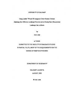
4 RESULTS AND DISCUSSION Fig. 2a illustrates a distinct seasonal pattern of average TS over the entire study area derived from MODIS-based 8-day composites. Also shown is a quadratic fit to the TS as a function of day of year. The observed seasonal pattern is consistent with other mid-latitude locations [15]. We also estimated TS for cloud-contaminated pixels based on the seasonal temperature trends as discussed in the Methods Section. But clearly there is no way to verify the accuracy of these values since the level and local occurrence of cloud formation is difficult to predict. However, we conducted a level of verification by artificially treating cloud-free cells as cloud contaminated and comparing their estimated TS with their actual values as shown in Fig. 2b. It revealed a strong relation between the estimated and actual surface temperatures (r2=88.3% with a slope of 0.86) and, consequently, demonstrated the potential of using the procedure for

Journal of Applied Remote Sensing, Vol. 1, 013511 (2007)

Page 5

estimating TS for cloud-contaminated pixels. However, in fact cloudy areas have lower maximum temperatures and predictions based on seasonal estimates (as we have done here) could have introduced some level of bias.

Fig. 2. (a) Seasonal pattern of average surface temperature over the entire study area; (b) comparison between estimated and actual surface temperature by artificially treating cloud-free cells as cloud contaminated.

Fig. 3 illustrates the relationship between the average tower-based TS for the MODIS image-acquisition period (between 10:30 am-12:00 pm local solar time) and daily mean tower-based TS derived from emitted longwave radiation measured at four sites from the southern commercial forest zone of Canada for 2004 and 2005 (including the NB NWL flux site). In general, the relationship was quite strong (r2 > 97%) emphasizing the generality of the relationship; some variation in equation slopes and intercepts, albeit small, existed. Our analysis suggested that our approach most likely would be applicable at regional scales.

Fig. 3. Relationship between average tower-based surface temperature between 10:30 am-12:00 pm period and daily mean temperatures at four flux sites across Canada, namely NB=New Brunswick (NWL), QC=Quebec, ON=Ontario, and SK=Saskatchewan.

We examined the seasonal patterns of MODIS-derived GDD at 1 km spatial resolution with respect to MODIS-based vegetation index-values, namely NDVI and EVI. To do this, we calculated the mean value of 8-day accumulated GDD, and 16-day accumulated NDVI and EVI for the entire study area and plotted their respective values as a function of day of year

Journal of Applied Remote Sensing, Vol. 1, 013511 (2007)

Page 6

(Fig. 4). Our analysis revealed that NDVI values saturated (reached a plateau) despite continued increases in GDD as shown in Fig. 4a. Tendencies of NDVI-values reaching saturation at the peak of growing season were corroborated by other researchers [8, 9]. In contrast, EVI values responded across the spectrum of seasonal changes in GDD (see Fig. 4b). Correlation between GDD and EVI was shown to be fairly strong, yielding an r2-value=87%. As a result of this correlation, the use of seasonally-averaged EVI values for enhancing the spatial resolution of GDD from 1 km to 250 m using data fusion techniques [14] was well justified (Fig. 5).

Fig. 4. Relationships between 8-day accumulated GDD and MODIS-based vegetation index-values [NDVI, graph (a) and EVI, graph (b)] as a function of day of year. Circled values in graph (a) highlight the tendency of NDVI-values to saturate at high GDD.

Fig. 5. Example of GDD values (a) at 1 km spatial resolution without data fusion, and (b) at 250 m spatial resolution with data fusion.

Fig. 6 shows a comparison between seasonal GDD averages derived from 101 climate stations of Environment Canada and corresponding three-year average of MODIS-derived values of GDD at 250 m spatial resolution. We found an offset of 511 GDD (Fig. 6) between values. This difference could be attributed to the following reasons: (i) The 8-day MODIS-based TS product was the average daytime TS obtained during the image-acquisition period during generally “cloud-free conditions”. As, the presence of cloud is non-uniform and occurs irregularly for a given area (and image), TS at a

Journal of Applied Remote Sensing, Vol. 1, 013511 (2007)

Page 7

pixel could be based on an average of TS for any number of non-cloudy days (within the 8-day period) in any 8-day composite of TS. As the temperature is normally higher on clear days, the MODIS-based 8-day composite of TS could have overestimated actual 8-day surface temperature averages, which would have contributed to a higher, non-representative calculation of GDD for many of the pixels. (ii) The estimation of TS for cloud-contaminated pixels could have positive bias as the estimated values are based on a mean seasonal trend, which could have led to higher estimates of GDD. (iii) The current MODIS-based estimates of GDD were for a warmer three-year period. 30-year Normals (1971-2000), because they represented averages, can conceal the influences of warmer years.

Fig. 6. Comparison of seasonal GDD derived from MODIS images and Environment Canada air temperature records for the 1971-2000 period.

Fig. 7a shows the long-term average of GDD derived from MODIS data and corrected based on the offset (-511 degree-days) between the two sets of values in Fig. 6. The average seasonal GDD was in the range of 1200-1800. We summarized the spatial pattern of GDD as follows: (i) High elevation areas, such as northwestern NB and the eastern part of NS had lower GDD in the 800-1400 range. This is consistent with the fact that high elevation areas are normally cooler than low elevation areas in summer. (ii) The areas along the coastlines had lower GDD at around 800-900 due to their proximity to cold ocean water. (iii) In general, GDD (and temperature) increased southward, as expected in the northern hemisphere. (iv) Land use patterns might also influence the observed GDD. For example, forested lands exhibited relatively cooler GDD with compare to agricultural lands due to the cooling effect associated with higher evapotranspiration rates in forested areas. For validation purposes, we generated a 30-year GDD map based on air temperatures from the 1951-1980 period from about 70 climate stations for 7 ecoregions in the province of NB (after Ref. 16, 17) as shown in Fig. 7b. The GDD values are categorized according to the colours shown in the legend in Fig. 7c. A comparison between GDD values from the 1951-1980 period and MODIS-image data over the 7 ecoregions of NB is shown in Fig. 7d. In relation to MODIS-derived GDD values, at least 75% of the area within the ecoregions falls within the reported ranges of GDD values [16] denoted along the y-axis of Fig. 7d. The comparison revealed that the spatial distribution of MODIS-derived GDD values had a similar and comparable pattern with the pattern of GDD values from the 1951-1980 period; the ranges for

Journal of Applied Remote Sensing, Vol. 1, 013511 (2007)

Page 8

individual ecoregions fall along the 1:1 correspondence line in Fig. 7d, except for ecoregion 4. Ecoregion 4, because of its proximity to cold water, demonstrated an abrupt temperature change from the coastline to the warmer interior (Fig. 7a). This feature was not wholly captured in the 1951-1980 period data [16; Fig. 7b], as data from only a few weather stations were available for the calculation of GDD.

Fig. 7. (a) Spatial distribution of long-term averaged MODIS-derived GDD, (b) GDD ranges for the different ecoregions of the province of NB (after Ref. 16, 17), (c) GDD categories according to colour, (d) comparison between GDD values from 1951-1980 period and MODIS-image data over the different ecoregions.

Journal of Applied Remote Sensing, Vol. 1, 013511 (2007)

Page 9

5 CONCLUDING REMARKS In this paper, we demonstrated the potential of using MODIS-based TS and EVI products for mapping the long-term average GDD for a significant portion of the Canadian Atlantic Maritime Ecozone. A simple method for the calculation of GDD was developed based on MODIS products and ancillary information, in particular, emitted longwave radiation from flux sites and GDD Normals from Environment Canada climate stations. This technique shows potential for predicting the temperature regime in the prediction of forest productivity. It also has potential to predict agricultural productivity in the province of PEI, where about 39% of the landbase is in crop production during the growing season.

Acknowledgments This study was partially funded by the Fluxnet-Canada Research Network (FCRN) project and funds from a Discovery Grant awarded to CPAB from the Natural Science and Engineering Council of Canada (NSERC). We would like to acknowledge NASA and Environment Canada for providing MODIS and GDD data free of charge. We also would like to thank Dr.’s Alan Barr, Andy Black, Hank Margolis, and Harry McCaughey for providing longwave radiation data from the Saskatchewan, Quebec, and Ontario flux sites. We also would like to express our appreciation for the helpful suggestions provided by two anonymous reviewers on an earlier version of the manuscript.

References [1]

[2] [3] [4]

[5] [6] [7] [8] [9]

C. P. -A. Bourque, F. -R. Meng, J. J. Gullison and J. Bridgland, “Biophysical and potential vegetation growth surfaces for a small watershed in northern Cape Breton Island, Nova Scotia, Canada,” Can. J. For. Res. 30, 1179–1195 (2000). [doi:10.1139/cjfr-30-8-1179] B. Li, S. Tao and R. W. Dawson, “Relations between AVHRR NDVI and ecoclimatic parameters in China,” Int. J. Rem. Sens. 23, 989–999 (2002). [doi:10.1080/014311602753474192] N. Lam, “Spatial Interpolation Methods: A Review," American Cartographer 10(2), 129-149 (1983). D. G. Goodin and G. M. Henebry, “A technique for monitoring ecological disturbance in tallgrass prairie using seasonal NDVI trajectories and a discriminant function mixture model,” Rem. Sens. Environ. 61, 270-278 (1997). [doi:10.1016/S0034-4257(97)00043-6] K. M. de Beurs and G. M. Henebry, “Land surface phenology, climatic variation, and institutional change: Analyzing agricultural land cover change in Kazakhstan,” Rem. Sens. Environ. 89, 497–509 (2004). [doi:10.1016/j.rse.2003.11.006] K. M. de Beurs and G. M. Henebry, “Land surface phenology and temperature variation in the International Geosphere–Biosphere Program high-latitude transects,” Global Change Bio. 11, 779–790 (2005). [doi:10.1111/j.1365-2486.2005.00949.x] S. R. Karlsen, A. Elvebakk, K. A. Høgda and B. Johansen, “Satellite-based mapping of the growing season and bioclimatic zones in Fennoscandia”, Global Ecol. Biogeogr. 15, 416-430 (2006). [doi:10.1111/j.1466-822X.2006.00234.x] X. Xiao, Q. Zhang, D. Hollinger, J. Aber and B. Moore, “Modeling gross primary production of an evergreen needleleaf forest using MODIS and climate data,” Ecol. Appl. 15, 954–969 (2005). A. R. Huete, H. Q. Liu, K. Batchily and W. van Leeuwen, “A comparison of vegetation indices over a global set of TM images for EOS–MODIS,” Rem. Sens. Environ. 59, 440–451 (1997). [doi:10.1016/S0034-4257(96)00112-5]

Journal of Applied Remote Sensing, Vol. 1, 013511 (2007)

Page 10

[10]

[11]

[12] [13] [14] [15] [16] [17]

A. Huete, K. Didan, T. Miura, E. P. Rodriguez, X. Gao and L. G. Ferreira, “Overview of the radiometric and biophysical performance of the MODIS vegetation indices,” Rem. Sens. Environ. 83, 195–213(2002). [doi:10.1016/S00344257(02)00096-2]. Ecological Stratification Working Group. A National Ecological Framework for Canada. Agriculture and Agri-Food Canada, Research Branch, Centre for Land and Biological Resources Research and Environment Canada, State of Environment Directorate, Ottawa/Hull, (1996). Q. K. Hassan and C. P.-A. Bourque, “Estimating daily evapotranspiration for forests in Atlantic Maritime Canada: application of MODIS imagery,” Proc. ASPRS, 11p. CD-ROM unpaginated (2006). T. R. Oke, Boundary Layer Climates, 2nd ed., Methuen, London and New York (1987). S. de Béthune, F. Muller and J. P. Donnay, “Fusion of multi-spectral and panchromatic images by local mean and variance matching filtering techniques,” Proc. 2nd Int. Conf.: Fusion of Earth Data, 31-36 (1998). F. K. Lutgens and E. J. Tarbuck, The Atmosphere, 8th ed., Prentice Hall, New Jersey (2001). P. A. Dzikowski, G. Kirby, G. Read and W. G. Richards, The climate for agriculture in Atlantic Canada, For the Atlantic Advisory Committee on Agrometeorology, Publication No. ACA 84-2-500, Agdex No. 070 (1984). The Ecosystem Classification Working Group. Our landscape heritage: the story of ecological land classification in New Brunswick. Department of Natural Resources and Energy, New Brunswick, Canada (2003).

Quazi K. Hassan is currently a PhD student and research assistant at University of New Brunswick. He received his BSc in electrical and electronic engineering from Khulna University of Engineering and Technology, Bangladesh, and MSc in remote sensing and GIS from University Putra, Malaysia. His research interests include use of optical and radar remote sensing into forestry-related applications, flood mapping and monitoring, land use mapping, river morphology, and coastal area mapping, among others. Charles P.-A. Bourque is Professor of forest hydrometeorology at University of New Brunswick. Dr. Bourque received his BSc (Hons) from Dalhousie University, Canada, in mathematics and theoretical ecology. He also received a second BSc in Dynamic Meteorology from the University of Alberta, Canada, an MSc and a PhD from University of New Brunswick, Canada in forest meteorology and environmental sciences. Dr Bourque’s research interests include systems modeling, eddy covariance measurement of biospheric fluxes, and landscape process modelling. Fan-Rui Meng is a Professor of forest watershed management at University of New Brunswick. Dr. Meng received a BSc in forest engineering and an MSc in forest planning from Northeast Forestry University, China, and a PhD in forest ecology from University of New Brunswick, Canada. Dr. Meng’s research interests include ecological modelling, forest watershed management, and forest hydrology. William Richards is a senior researcher with Adaptation and Impacts Research Division (AIRD) of Environment Canada and is based at the University of New Brunswick. He received a BSc (Hons) in Physics from University of New Brunswick, Canada and an MSc in Atmospheric Physics from University of Toronto, Canada. Mr. Richards’ research interests

Journal of Applied Remote Sensing, Vol. 1, 013511 (2007)

Page 11

include applied climatology, remote sensing, climate and climate change impacts and adaptation.

Journal of Applied Remote Sensing, Vol. 1, 013511 (2007)

Page 12