Water 2015, 7, 1889-1920; doi:10.3390/w7051889
OPEN ACCESS
water ISSN 2073-4441 www.mdpi.com/journal/water Article
Spatial Quantification of Non-Point Source Pollution in a Meso-Scale Catchment for an Assessment of Buffer Zones Efficiency Mikołaj Piniewski 1,†, *, Paweł Marcinkowski 1 , Ignacy Kardel 1 , Marek Giełczewski 1 , 2,3 Katarzyna Izydorczyk 2 and Wojciech Fratczak ˛ 1
Department of Hydraulic Engineering, Warsaw University of Life Sciences (WULS-SGGW), Nowoursynowska str. 159, Warszawa 02-776, Poland; E-Mails:
[email protected] (P.M.);
[email protected] (I.K.);
[email protected] (M.G.) 2 European Regional Centre for Ecohydrology of the Polish Academy of Sciences, Tylna str. 3, Łód´z 90-364, Poland; E-Mails:
[email protected] (K.I.);
[email protected] (W.F.) 3 Regional Water Management Authority in Warsaw, 13B Zarzecze, Warszawa 03-194, Poland †
Current address: Potsdam Institute for Climate Impact Research (PIK), P.O. Box 60 12 03, Potsdam 14412, Germany.
* Author to whom correspondence should be addressed; E-Mail:
[email protected]; Tel.: +49-331-2882-0721. Academic Editors: Lutz Breuer and Philipp Kraft Received: 2 February 2015 / Accepted: 3 April 2015 / Published: 27 April 2015
Abstract: The objective of this paper was to spatially quantify diffuse pollution sources and estimate the potential efficiency of applying riparian buffer zones as a conservation practice for mitigating chemical pollutant losses. This study was conducted using a semi-distributed Soil and Water Assessment Tool (SWAT) model that underwent extensive calibration and validation in the Sulejów Reservoir catchment (SRC), which occupies 4900 km2 in central Poland. The model was calibrated and validated against daily discharges (10 gauges), NO3 -N and TP loads (7 gauges). Overall, the model generally performed well during the calibration period but not during the validation period for simulating discharge and loading of NO3 -N and TP. Diffuse agricultural sources appeared to be the main contributors to the elevated NO3 -N and TP loads in the streams. The existing, default representation of buffer zones in SWAT uses a VFS sub-model that only affects the contaminants present in surface runoff.
Water 2015, 7
1890
The results of an extensive monitoring program carried out in 2011–2013 in the SRC suggest that buffer zones are highly efficient for reducing NO3 -N and TP concentrations in shallow groundwater. On average, reductions of 56% and 76% were observed, respectively. An improved simulation of buffer zones in SWAT was achieved through empirical upscaling of the measurement results. The mean values of the sub-basin level reductions are 0.16 kg NO3 /ha (5.9%) and 0.03 kg TP/ha (19.4%). The buffer zones simulated using this approach contributed 24% for NO3 -N and 54% for TP to the total achieved mean reduction at the sub-basin level. This result suggests that additional measures are needed to achieve acceptable water quality status in all water bodies of the SRC, despite the fact that the buffer zones have a high potential for reducing contaminant emissions. Keywords: water quality; nutrient; ecotones; vegetative filter strips; buffer strips; hydrological model; Pilica; diffuse pollution
1. Introduction 1.1. Water Management Context Fulfilling the requirements of the European Water Framework Directive [1] and the Nitrates Directive [2] by reducing pollution emissions to water ecosystems remains a major challenge faced in water management. Particularly, the main issue is the reduction of non-point pollution that originates from agricultural land. The contributions of agriculture to the pool of nitrogen and phosphorus compounds in water ecosystems are high. In Poland, the large share of farmland consisting of highly fragmented arable land and strongly dispersed developments has resulted in major pressure from pollution emission sources, including (1) pressure from agriculture related to the use of inappropriate farming practices (transport of organic and mineral nitrogen and phosphorus compounds from fertilizers to the environment) and (2) pressure from scattered households that are not connected to sewage systems. Thus, the development of N and P reduction strategies is a major task for water authorities throughout Europe. One example of activities that are undertaken to achieve sustainable water management goals in agricultural catchments is the EU-funded EKOROB project (Ecotones for reducing diffuse pollution). The main objective of this project is to develop an Action Plan for reductions of diffuse pollution in the Pilica River catchment (Poland) and will help achieve a good ecological status for the water in the Sulejów Reservoir, particularly by reducing eutrophication and decreasing the frequency and intensity of cyanobacterial blooms. The Action Plan is based on the ecohydrology concept [3–5], which assumes that the basis for integrated river basin management is the quantification of catchment-scale processes that are part of the hydrological cycle. The concept of ecohydrology involves quantifying hydrological processes at the basin scale and the entire hydrological cycle to quantify ecological processes. This quantification includes the patterns of hydrological pulses along the river continuum and the identification of various
Water 2015, 7
1891
human impacts on point and non-point sources of pollution [6]. Thus, this quantification should be the first step when developing regulatory processes for sustainable water use and ecosystem protection. Although many mathematical tools are available for this task, the Soil and Water Assessment Tool (SWAT) [7] is one of the most widely used and comprehensive tools. 1.2. The Use of SWAT for Quantifying Emission Sources SWAT is a comprehensive hydrological/water quality model that is increasingly being used to address a wide variety of water resource problems across the globe [8]. Several studies have investigated the spatial variability and distribution of various pollutant emissions/losses in catchments of different sizes [9–12]. Niraula et al. [9] calibrated SWAT (and a less complex GWLF model) for a small catchment in Alabama and used it to identify Critical Source Areas (CSAs) for sediment, TN and TP based on the loadings per unit area (yield or emission or losses) at the sub-basin level. Another application of SWAT in a medium-sized Greek catchment resulted in similar findings, but with a finer level of Hydrological Response Units (HRUs) [10]. Wu and Chen [11] investigated the influences of point source and diffuse pollution on the water quality of a relatively large catchment in south China by using SWAT. These authors concluded that diffuse pollution overwhelmingly surpasses point source pollution for all constituents except TP. In addition, these authors identified CSAs at the HRU and sub-basin levels. Finally Wu and Liu [12] calibrated SWAT for a large catchment in Iowa and showed a relationship between the shares of agricultural areas with sediment and NO3 -N emissions by using the calibrated model. 1.3. Riparian Buffer Zones and Their Modeling in SWAT Riparian buffer zones (ecotones, vegetative filter strips) are an effective Best Management Practice (BMP) for buffering aquatic ecosystems against nutrient losses from the agricultural landscapes. Buffer zones are strips of permanent vegetation (including herbs, grasses, shrubs or trees) that are adjacent to aquatic ecosystems and used to maintain or improve water quality by trapping and removing various non-point source pollutants from overland and shallow sub-surface flow [13–16]. For pollutants transported in surface runoff, the process of sediment and nutrient trapping by buffer zones is reasonably well understood, particularly for grass filter strips (cf. review [17]). Reductions in the surface flow velocities due to the increased hydraulic roughness of the vegetation in the buffer enhanced particle deposition. Vought et al. [18] reported that a buffer strip with a width of 10 m can reduce phosphorus loads, which are typically bound to sediments, by as much as 95%. Buffer zone are effective for removing sediments and other suspended solids contained in surface runoff; however, soluble forms of nitrogen and phosphorus are not removed as effectively as sediments [19]. Results collected from 44 fields (row crops with slopes range from 1%–14%) showed that a 10-m buffer zone reduced the total suspended solids, soluble phosphorus and nitrate-nitrogen contents by 64%, 34% and 38%, respectively [20]. The efficiencies of narrow buffer zones (5–10 m) in Norway varied from 81%–91%, 60%–89% and 37%–81% for particles, total phosphorus and total nitrogen, respectively [21]. Buffer strips are normally less efficient for removing nitrate than orthophosphates from surface runoff. In contrast with orthophosphate, nitrogen is very labile and is not largely adsorbed within the soil [18].
Water 2015, 7
1892
However, the impacts of the sub-surface flow efficiency of the buffer zones on reducing nitrogen are well described in the literature and often reach a concentration reduction of 90% [17]. A meta-analysis of nitrogen removal in riparian buffers based on data from 65 individual riparian buffers from published studies indicated a mean removal effectiveness of 76.7% [22]. However, the efficiency of buffer zones for reducing phosphorus in shallow groundwater is not well documented, and some studies suggest that riparian zones are ineffective for removing dissolved phosphorus or could even release phosphorus to the water [23,24]. Buffer zones along small streams that are more exposed to pressure from agriculture are more efficient than buffer zones along larger rivers. A key factor for determining the efficiency of buffer zones is their continuity. Continuous and narrow riparian buffers are more efficient than wider and intermittent buffers [25]. Hence, an important issue for effective water management is the selection of priority areas that have the highest emissions of diffuse pollution. Next, concentrating measures, such as buffer zones, should be applied in these areas. Catchment-scale water quality modeling is one possible solution for quickly identifying priority areas. Numerous examples are available regarding the application of SWAT for simulating the affects of buffer zones on diffuse pollution [26–29]. Older versions of SWAT used a very simplistic equation that was only based on filter width for calculating the HRU-level reduction rate of buffer zones. This equation was based on empirical data from the US regarding buffer strip efficiency [27,28]. Since then, SWAT has undergone certain modifications to address variable source areas within watersheds and vegetated buffers adjacent to streams [26,30]. The new VFS sub-model currently used in SWAT reduces the sediment, nitrate and phosphorus loading in streams as a function of estimated reductions in runoff. Hence, the new VFS sub-model only affects contaminants present in surface runoff and neglects nutrient trapping in shallow groundwater. As mentioned previously for nitrogen in sub-surface flow, buffer zones are very efficient measures [17]. However, little consensus has been reached for phosphorus [23,24]. This result suggests that the buffer zone efficiency is case-specific and depends on local conditions. Hence it is equally as important to apply existing models as it is to measure the efficiency of existing buffer zones in the field to gain more confidence regarding their behavior. 1.4. Objective Two objectives of this paper are: 1. Spatial quantification of NO3 -N and TP emissions from major pollution sources in a meso-scale catchment using SWAT. 2. Simulation of buffer zone effects on the mitigation of pollution losses when applied in Critical Source Areas through the combined use of the default SWAT VFS sub-model and local field monitoring data. The term “meso-scale catchment” refers to catchments with an order of magnitude between 10 and 103 km2 [31]. A part of the Pilica catchment selected as the case study in this paper, a demonstration catchment of the EKOROB project, satisfies this condition.
Water 2015, 7
1893
2. Materials and Methods 2.1. Study Area The study was conducted in the Sulejów Reservoir catchment (hereafter referred to as the SRC). Sulejów is a shallow and eutrophic artificial reservoir that was built in 1974 and is situated in the middle course of the Pilica River in central Poland. Two main tributaries supply water to the Sulejów Reservoir: the Pilica and Lucia˛z˙ a Rivers. At its full capacity, this reservoir covers an area of 22 km2 , with a mean depth of 3.3 m and a volume of 75 × 106 m3 . The Sulejów Reservoir was used as a drinking water reservoir for Łód´z agglomeration until 2004 and is currently an important recreational site that has been extensively studied (cf. review [32]). Microcystis aeruginosa is the dominant species of bloom-forming cyanobacteria in the reservoir and produces microcystin-LR, microcystin-YR, and microcystin-RR [33–35]. The SWAT model is used in this study for the entire SRC area upstream of the dam, which occupies 4933 km2 (Figure 1). This area consists of the Pilica (contributing 79.8% of area) and the Lucia˛z˙ a (15.3%) River catchments and a direct reservoir sub-catchment with several smaller streams (4.9%). The elevation of the SRC varies from 154 m in the lowland areas in the north to 499 m in the highland areas in the south. The distribution of land cover in the SRC area is as follows: 44.4% arable land, 38.6% forest areas, 12.3% grasslands, and 4.7% urban areas (mainly low-density residential areas), with the remaining land occupied by other types of land cover (data according to Corine Land Cover 2006). The predominate soil types in this area are loamy sands and sands. The climate of this area is typical for central Poland, with a mean annual temperature of 7.5 ◦ C and mean January and July temperatures of −4 ◦ C and 18 ◦ C, respectively. The mean annual precipitation is 600 mm. The highest amounts of precipitation occur in June/July, and the lowest amounts of precipitation occur in January. The flow regime is characterized by early spring snow-melt induced floods and summer low flows with occasional summer floods. The quantitative pressure on surface water resources is relatively low. The fish farming industry scattered around the catchment and the Cieszanowice Reservoir constructed in 1998 on the Lucia˛z˙ a River (volume of 7.3 × 10 m3 at full capacity) are the only considerable sources of flow alteration. In contrast, multiple point and non-point pollution sources in the area result in elevated N and P loads flowing into the Sulejów Reservoir, which eventually contribute to toxic cyanobacterial blooms in its waters. These different sources will be described systematically in terms of SWAT model inputs in Sub-Section 2.4. 2.2. SWAT Model 2.2.1. General Features SWAT is a physically based, semi-distributed, continuous-time model that simulates the movement of water, sediment, and nutrients on a catchment scale with a daily time step. The basic calculation unit, referred to as a “hydrological response unit” (HRU) is a combination of land use, soil, and slope overlay. Both water balance components, which is a driving force behind affect all processes that occur in a
Water 2015, 7
1894
watershed, and water quality, output parameters are computed separately for each HRU. Water, nutrients and sediment leaving HRUs are aggregated at the sub-basin level and routed through the stream network to the main outlet to obtain the total flows and loadings for the river basin.
Figure 1. Study area. In this study, channel routing was modeled using a variable storage coefficient approach. The modified USDA Soil Conservation Service (SCS) curve number method for calculating surface runoff and the Penman-Monteith method for estimating potential evapotranspiration (PET) were selected. In the model, snow-melt estimations are based on the degree-day method. The SWAT adapted plant growth model, which is used to assess the removal of water and nutrients from the root zone, transpiration, and biomass/yield production, is based on EPIC [36]. The in-stream water quality component allows us to
Water 2015, 7
1895
control nutrient transformations in the stream. The in-stream kinetics used in SWAT for nutrient routing are adapted from QUAL2E [37]. SWAT simulates the movement and transformation of several forms of nitrogen and phosphorus in the watershed. In the nitrogen cycle, the main processes are denitrification, nitrification, mineralization, plant uptake, decay, fertilization, and volatilization. In the phosphorus cycle, the main processes are mineralization, fertilization, decay, and plant uptake. The nutrient transport pathways from upland areas to stream networks correspond to the following hydrological transport pathways: surface runoff, lateral subsurface flow and groundwater flow. Additionally point source discharges of water and contaminants can be defined that are directly input into the water routed through the stream network. From the point of view of modeling buffer zones in SWAT, it is important to note that HRUs are lumped and non-contiguous geographic units within each sub-basin. A SWAT model setup may consist of thousands of such units, and each of them may represent one field, a portion of a field, or, more likely, portions of many fields [38]. 2.2.2. Runoff-Reduction-Based Buffer Zone Sub-Model A key characteristic of the buffer zone sub-model implemented in SWAT is that it works at the HRU level and reduces the loads of sediment, nitrate and phosphorus that enter the stream as a function of estimated reductions in runoff. Hence, the sub-model only affects contaminants that are present in surface runoff and neglects the potential affects of buffer zones on shallow groundwater. This sub-model was developed and evaluated using measured data derived from the literature and included data that were collected using differing experimental protocols and under conditions with different soils, slopes and rainfall intensities. When measured data were unavailable, predictions from the process-based Vegetative Filter Strip MODel (VFSMOD) [39] and its companion program, UH, were used. The UH (upland hydrology) utility uses the curve number approach (USDA-SCS, 1972), unit hydrograph and the Modified Universal Soil Loss Equation (MUSLE) [40] and allowed us to generate a database of sediment and runoff loads that enter the VFS. VFSMOD simulations were used to evaluate the sensitivities of various parameters and correlations between the model inputs and predictions. Consequently, an empirical model for runoff reduction by VFSs was developed, as described by the following equation: RR = 75.8 − 10.8 ln(RL ) + 25.9 ln(Ksat )
(1)
where RR is the runoff reduction (%); RL is the runoff loading to the buffer zone (mm); and Ksat is the saturated hydraulic conductivity (mm · h−1 ). An important consideration is that SWAT conceptually partitions VFS sections within an HRU into two parts: a short part that occupies 10% of its length and receives flow from the 0.25–0.75 of the field area and a part that occupies 90% of its length and receives the remaining amount of flow. A fraction of the flow through the most heavily loaded 10% that is fully channelized is not subject to the VFS sub-model. Although the buffer zone width is an essential and intuitive characteristic that influences its trapping efficiency, it is not implemented as a parameter of the VFS sub-model in SWAT. Instead, the drainage area to buffer zone area ratio (DAF Sratio ) that is negatively correlated with the buffer zone width is combined with the HRU-level predicted runoff to estimate RL .
Water 2015, 7
1896
The sediment reduction model based on VFS data removes sediment by reducing runoff velocity and enhancing infiltration in the VFS area, which is described by the following equation: SR = 79.0 − 1.04SL + 0.213RR
(2)
where SR is the predicted sediment reduction (%) and SL is the sediment loading (kg · m−2 ). The nitrate reduction model was only based on runoff reduction, as described by the following equation: N NR = 39.4 + 0.584RR (3) where N NR is the reduction of nitrate nitrogen (%). The model for total phosphorus reduction was based on sediment reduction, which is described by the following equation: T PR = 0.9SR (4) where T PR is the total phosphorus reduction (%); and SR is the sediment reduction (%). 2.3. SWAT Setup of the SRC Table 1 lists all major data items and sources used to create the SWAT model setup of the SRC. The specific applications of this data at different stages of model development are described below. Table 1. Data items and sources used to create the SWAT model setup of the SRC. Data
Source
Digital Elevation Model Water cadastre GIS layers Corine Land Cover 2006 Orthophotomap Agricultural statistics Agricultural soil map 1:100,000
CODGiK (Central Agency for Geodetic and Cartographic Documentation) RZGW (Regional Water Management Authority in Warsaw) GDOS (General Directorate of the Environmental Protection) GUGiK (Head Office of Geodesy and Cartography: geoportal.gov.pl) The Local Data Bank of GUS (Central Statistical Office) IUNG-PIB (Institute of Soil Science and Plant Cultivation - National Research Institute) RDLP (Regional Directorate of State Forests in Łód´z, Radom and Katowice) GIOS (Chief Inspectorate of Environmental Protection IMGW-PIB (Institute of Meteorology and Water Management - National Research Institute)
Forest soil maps 1:25,000 Atmospheric deposition of nitrogen Climate data
The automatic watershed delineation of the SRC was based on the Digital Elevation Model (DEM) and stream network GIS layer. A 5 m resolution DEM characterized by a mean elevation error of 0.8–2.0 m was created from the ESRI TIN DEM available from CODGiK (Polish Central Geodetic and Cartographic Agency). This DEM resulted in the division of the catchment into 272 sub-basins with average areas of 18.1 km2 (Figure 2). The Corine Land Cover (CLC) 2006 layer was used as the primary data source for the land use/land cover map. However, this layer was enhanced by several supplementary datasets and analyses:
Water 2015, 7
1897
• The (open) drainage ditch layer was used to sub-divide the CLC grasslands class into those under (code: FES2) and beyond (code: FESC; cf. Figure 3) the influences of drainage. It was assumed that the influences of the drainage ditches occurred within a 100 m buffer around the ditches. • The orthophotomap was used to identify which SWAT crop database classes should be assigned to the “Heterogeneous agricultural areas” CLC class (code 2.4). Based on a manual, case-by-case investigation, the following three classes were most frequently assigned: “Agricultural land generic” (AGRL), “Urban low density” (URLD) and “Mixed forests” (FRST). • The commune-level (39 units) agricultural census statistical data from 2010 were used to sub-divide the “Non-irrigated arable land” CLC class (code 2.1.1) into classes that represented particular crops that were cultivated in the SRC. This subdivision was done using a set of GIS techniques, including the “Create Random Raster” tool in ArcGIS. Thus, a 100 m resolution raster dataset that represented the random (yet preserving the commune level of crop distribution) locations of 6 major crops was created and combined with the final land cover map used as SWAT input. Although it may seem risky to generate random crop locations, we believe that this approach does not significantly impact the modeling result due to the lumped nature of the HRUs within each sub-basin. Overall, the following five crops were distinguished as well as a fallow/abandoned land class (BERM): spring barley (BARL), rye (RYE), potato (POTA), corn silage (CSIL) and head lettuce (LETT). Figure 3 shows the final distributions of all land cover classes in the SWAT model setup. The numerical soil map (scale 1:100,000) from the Institute of Soil Science and Plant Cultivation (IUNG) and numerical soil maps (scale 1:25,000) from the Regional Directorate of State Forests were used to create a user soil input map with 27 soil classes. By overlaying the land use and soil maps, 3401 HRUs were delineated in the catchment. The following area thresholds were used in the HRU delineation: 30 ha for land cover and 50 ha for soils. Thus, when using this method, all land cover types below the first threshold in each sub-basin were removed and aggregated into the remaining classes. The meteorological data required by SWAT (precipitation, solar radiation, relative humidity, wind speed, and maximum and minimum temperatures) were acquired from the Institute of Meteorology and Water Management-National Research Institute (IMGW-PIB) for 1982–2011. Precipitation data were obtained from 49 stations, whereas data for other variables from 17 stations. To improve the spatial representation of climate inputs, spatial interpolation of all variables (apart from solar radiation, which was only available for one station) was performed before reading the SWAT input files. For precipitation, the Ordinary Kriging (OK) method was applied. However, the Inverse Distance Weighted method was used for the other variables. Szcze´sniak and Piniewski [41] showed that the OK method outperforms the SWAT default method for precipitation. For other weather variables, the interpolation process did not significantly affect the modeling results. 2.4. Pollution Sources in the Model Setup Parameterization of point and non-point source pollution plays a critical role in water quality modeling and has attracted considerable attention in this paper. The following anthropogenic pollution sources
Water 2015, 7
1898
were identified: (1) diffuse pollution from agricultural areas; (2) sewage treatment plants and septic tanks and (3) fish ponds. Atmospheric deposition of nitrogen was also considered.
Figure 2. Delineation of the SRC into sub-basins and the gauging station locations used for calibration and validation. 2.4.1. Atmospheric Deposition The mean concentration of nitrogen in precipitation measured in Sulejów near the inlet of the Sulejów Reservoir was obtained from the Chief Inspectorate of Environmental Protection (GIOS). The monthly results covered the time period of 1999–2010. Precipitation samples were collected daily, and an integrated sample was created and measured in the laboratory each month. Between 1999 and 2010, the mean annual concentrations varied significantly between 1.39 and 2.2 mg N · L−1 . The final value input into the model was subject to calibration and equaled 1.48 mg N · L−1 .
Water 2015, 7
1899
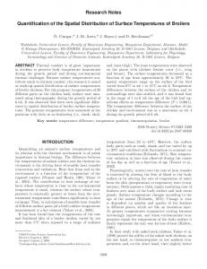
Figure 3. Land cover classes used as input for the SWAT model of the SRC. All codes as in the default SWAT plant database with one exception: FES2 has the same parameters as FESC, but is under the influence of open drainage ditches. 2.4.2. Fertilizers Diffuse N and P pollution from agricultural fields mainly results from fertilizer use. SWAT enables us to define crop- and soil-specific management practices scheduled by date for each agricultural HRU. Typical management practice schedules, including the dates, types and amounts of fertilization, were obtained by consulting local extension service experts. First, derived management schedules were assigned to agricultural HRUs by using the ArcSWAT interface. However, this approach typically leads to bias in the total amounts of spatially-averaged fertilizer when compared with data from external sources. In this study, we used commune-level data from the Central Statistical Office (as for 2010) to determine mineral fertilizer use and livestock population. The livestock population was used to calculate the amount of available organic fertilizer (manure or slurry). In the final step conducted using GIS software, correction factors for fertilizer rates were defined for the sub-basins that overlapped with different communes. The commune layer intersected the sub-basin layer so that the total amounts of fertilizer used annually in different communes (expressed in tons of N and P) could be distributed over the SWAT sub-basins proportionally to the area of agricultural land in each sub-basin. Simultaneously, we aggregated the total fertilizer use per sub-basin from the model output based on initially implemented management schedules. Next, correction factors were calculated for each sub-basin as the ratios of total fertilizer use at the sub-basin level from census data to the total fertilizer use obtained from the SWAT output files. In the final step, each HRU fertilizer rate in the operation schedules was adjusted using the calculated correction factors. After this adjustment, the bias in the spatially averaged amounts of fertilizer largely decreased. Figure 4 shows the final, sub-basin-averaged rates of mineral and organic fertilizers applied in the SWAT model of the SRC.
Water 2015, 7
Figure 4. Sub-basin-averaged N and P fertilizer rates: (A) mineral nitrogen; (B) organic nitrogen; (C) mineral phosphorus; (D) organic phosphorus.
1900
Water 2015, 7
1901
2.4.3. Sewage Twenty three sewage treatment plants discharging an average of more than 2 L · s−1 of treated sewage water annually were identified in the SRC and used in the model setup (Figure 5A). The largest plant of the SRC situated in Piotrków Trybunalski discharges its sewage water downstream of the Sulejów Reservoir and was therefore neglected during model setup. For each sewage treatment plant, discharge and nutrient loads were expressed as constant or mean monthly values depending on the available data. These values were obtained directly from plant operators in most cases by using a telephone/electronic survey.
Figure 5. Sewage treatment plants (A) and fish ponds (B). Even though water management in Poland is undergoing rapid modernization, which is manifested, for example, by investments in treatment plants, many rural and suburban areas remain disconnected from sewer systems. In such cases, domestic septic systems are usually used for sewage treatment. However, one common problem associated with domestic septic systems in Poland is leaking septic tanks [42]. The SWAT model uses a biozone algorithm [43] to simulate the effects of on-site wastewater systems. The type of septic tank widely used in Poland can be approximately represented by the so-called “failing systems” in SWAT. To identify approximate locations of septic systems in the SRC, commune-level data for the number of people disconnected from wastewater treatment plants were used, which were obtained from the Local Data Bank of the Central Statistical Office (GUS). This number was
Water 2015, 7
1902
estimated as 229,000 people for the entire SRC. Spatial analysis of these data made it possible to identify 202 HRUs with the land cover classes “URLD” (urban low density) or “URML” (urban medium-low density), in which the septic function was initiated (Figure 5A). The water quality parameters of the sewage effluents were specified based on the available literature [44]. For example, the TN and TP concentrations were 60 mg · L−1 and 20 mg · L−1 , respectively. 2.4.4. Fish Ponds An important feature of the SRC is carp breeding in earth ponds at traditional land-based farms adjacent to the river channels. The area of ponds identified in the 32 sub-basins was significant (Figure 5B). The ponds were represented in SWAT by defining monthly water use parameters (water withdrawn from the reaches of the river for filling the ponds in the spring and maintaining the desired water level until late summer) and point source discharges (representing water release to adjacent reaches of the river in October to empty the ponds before winter). The quantities of the abstracted and released water were calculated based on the estimated pond volume. The water quality characteristics of the discharged water remain largely unknown. Thus, a literature review of the effects of carp breeding on water quality in Central Europe [45,46] was used to define the mean concentrations of the different constituents in the released water: 2.96 mg TN · L−1 and 0.7 mg TP · L−1 . 2.4.5. Summary Table 2 lists three main anthropogenic point pollution sources and quantifies the mean annual TN and TP loads that originated from these sources and entered the stream network of the SRC. These estimates are very uncertain for each pollution source. The quantity of released water and the TN and TP concentrations both vary temporally and spatially. Table 2 shows that the order of magnitude is the same for all variables. For TN, the loads from the sewage treatment plants are slightly greater than those from the septic tank effluent and fish pond releases. For TP, the fish pond releases are the major source and the treatment plants and septic tanks are the second and third sources, respectively. However, in our opinion, the TP load from septic tank effluents is underestimated because SWAT does not simulate the downward movement of P to the groundwater. In addition, while the loads from treatment plants (in SWAT) are usually constant with time, the loads from the fish ponds only occur in October. In contrast, the loads from septic tank effluents are variable with time because the travel time between the bottom of the tank to the nearest river depends on the soil physical properties and hydrological conditions. Table 2. Mean annual TN and TP loads entering the stream network in the SRC that originated from different pollution sources. Pollution Source
TN (kg/year)
TP (kg/year)
Sewage treatment plants Septic tank effluent Fish pond releases
81,989 65,572 53,313
6,913 1,462 9,273
Total
200,874
17,648
Water 2015, 7
1903
Table 2 does not include the loads from the two remaining sources of atmospheric deposition and agricultural production. Because these sources are land-based sources, the load that enters the soil profile is generally known (e.g., Figure 4) but the load that enters the stream network is not. The load that enters the stream network is definitely smaller than the load entering the soil profile due to soil retention, plant uptake etc., and its direct estimation would require modeling. 2.5. Spatial Calibration Approach SWAT-CUP is a program that allows to use a number of different algorithms to optimize the SWAT model. In addition, SWAT-CUP can be used for sensitivity analysis, calibration, validation and uncertainty analysis [47]. In this paper, we applied SWAT-CUP version 2009 4.3 and selected the optimization algorithm SUFI-2 (Sequential Uncertainty Fitting Procedure Version 2), which is an inverse modeling program that contains elements of calibration and uncertainty analysis [48]. Although SUFI-2 is a stochastic procedure, it does not converge with any “best simulation” and quantifies standard goodness-of-fit measures, such as the Nash-Sutcliffe Efficiency (NSE) or R2 for each model run. Hence, SUFI-2 indicates the “best simulation” among all of the performed runs, which corresponds to the run with the highest/lowest value of the earlier defined objective function. In this study, we used the widely used NSE as an objective function. The NSE can range from −∞ to 1, where 1 is optimal. Moriasi et al. [49] recommended the value of 0.5 as the threshold for satisfactory model performance for a monthly time step, mentioning that under certain circumstances (e.g., daily time step, high uncertainty of observations) this requirement could be made less stringent. We also tracked other goodness-of-fit values, such as R2 and percent bias (PBIAS). The PBIAS measures the average tendency of the modeled data to be larger or smaller than their observed counterparts. Positive values indicate model underestimation bias, and negative values indicate model overestimation bias. Calibration was performed in three steps, beginning with continuous daily discharge, continuing with irregular (approximately one measurement per month) and daily NO3 -N loads and ending with TP loads. The calibration period was from 2006 to 2011, and the validation period was from 2000 to 2005. Figure 2 presents the locations of the 10 flow gauging stations (data acquired from IMGW-PIB) and 7 water quality monitoring stations (concentration data acquired from the General Inspectorate of Environmental Protection), from which the time series were used for calibration and validation. The average daily loads (kg · day−1 ) on the sampling dates were calculated based on observed daily discharge data (m3 · day−1 ) at the closest flow gauging station. If the flow gauging station was situated at another location than the water quality station, discharge data were scaled using catchment area ratios. We evaluated the relationships between the NO3 -N and TP concentrations and discharge for all studied gauges and concluded that the correlations were too low (median R2 equal to 0.2 for NO3 -N and 0.03 for TP) to use any regression-based methods for continuous load estimation. Three parameter sets, one for discharge, one for NO3 -N, and one for TP, and their initial ranges applied in SUFI-2 (Electronic Supplement, Tables S1–S3) were chosen based on the previous applications of the SWAT model under Polish conditions [41,50,51], and on the sensitivity analysis performed in the SRC. In most SWAT studies, calibration is restricted to the catchment outlet. In some cases, especially in small (i.e.,