Spatially coherent latent topic model for concurrent object segmentation and classification Liangliang Cao Dept. of Electrical and Computer Engineering University of Illinois at Urbana-Champaign (UIUC), USA
Li Fei-Fei Dept. of Computer Science Princeton University, USA
[email protected]
[email protected]
Abstract We present a novel generative model for simultaneously recognizing and segmenting object and scene classes. Our model is inspired by the traditional bag of words representation of texts and images as well as a number of related generative models, including probabilistic Latent Sematic Analysis (pLSA) and Latent Dirichlet Allocation (LDA). A major drawback of the pLSA and LDA models is the assumption that each patch in the image is independently generated given its corresponding latent topic. While such representation provide an efficient computational method, it lacks the power to describe the visually coherent images and scenes. Instead, we propose a spatially coherent latent topic model (Spatial-LTM). Spatial-LTM represents an image containing objects in a hierarchical way by oversegmented image regions of homogeneous appearances and the salient image patches within the regions. Only one single latent topic is assigned to the image patches within each region, enforcing the spatial coherency of the model. This idea gives rise to the following merits of Spatial-LTM: (1) Spatial-LTM provides a unified representation for spatially coherent bag of words topic models; (2) Spatial-LTM can simultaneously segment and classify objects, even in the case of occlusion and multiple instances; and (3) SpatialLTM can be trained either unsupervised or supervised, as well as when partial object labels are provided. We verify the success of our model in a number of segmentation and classification experiments.
1. Introduction Understanding images and their semantic contents is an important and challenging problem in computer vision. In this work, we are especially interested in simultaneously learning object/scene category models and performing segmentation on the detected objects. We present a novel generative model for both unsupervised and supervised classification. In recent years, bag of words models (e.g., probabilistic
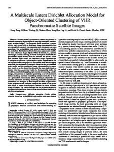
A. Input Image
E. Coherent regions for Spatial-LTM
B. LDA initialized topics
F. Spatial-LTM initialized topics
C. LDA learned topics D. LDA learned object
G. Spatial-LTM learned topics
H. Spatial-LTM segmentation results
Figure 1. (This figure must be viewed in colors) Comparison of the bag of words model and our proposed model, Spatial-LTM. Panel A shows the original input image. Panel E shows the input regions to Spatial-LTM provided by a over-segmentation method. Panels B and F in Column 2 illustrate the initial latent topic assignments to the image patches by either the traditional bag of words model (LDA) or Spatial-LTM. The circles denote the visual words provided by local interest point detectors. Different colors of the circles denote different latent topics of the patch. Panels C and G in Column 3 illustrate the latent topic assignments after the models have learned the object classes. Most of the patches on the human face are colored in red, indicating that the models have successfully recognized object. Finally, Panel D and H in Column 4 show the segmentation results of LDA and Spatial-LTM respectively. One can see that by encoding the spatial coherency of the image patches, Spatial-LTM achieves a much better segmentation of the object.
Latent Sematic Analysis (pLSA) [13] and Latent Dirichlet Allocation (LDA) [2]) have shown much success for text analysis and information retrieval. Inspired by this, a number of computer vision works have demonstrated impressive results for image analysis and classification [6, 7, 27, 11, 25, 22, 20] using the bag of words models. Such models are attractive due to the computational efficiency and their ability of representing images and objects with dense patches. This is achieved by an assumption in bag of words models where the spatial relationships of the image patches or object parts are ignored. In contrast, object
models that explicitly encode spatial information among the parts or regions usually require formidable computational costs in inference [12, 10, 16], forcing these algorithms to often represent objects with a very few number of parts. One should observe, however, there is a distinct difference between image and text analysis: there are no natural visual analogues of words. In other words, text documents are naturally composed of distinctive vocabularies while there is no such obvious word-level representation in images. To borrow the algorithms from text analysis, the researchers usually employ various local detectors [15, 23], and describe them as “visual words” that play the role of vocabulary words in the bag of words model. Although modern local detectors and descriptors offer powerful characterization of images, the bag of visual words representation resulted from these detectors have some inherent weaknesses. First, detected regions on an image are often sparse, leaving many uncovered areas of the images. When one is interested in segmentation, this kind of sparsity is detrimental to the eventual results. Second, spatial relationships among the different parts of an image are often critical in visual recognition tasks. A scrambled collection of patches from a car image does not necessarily evoke the recognition of a car. The current bag of words representation ignores this important issue, hence affecting the final accuracy of the recognition tasks. In this paper, we would like to inherit the strength of the bag of words representation, and improve it by incorporating meaningful spatial coherency among the patches. In traditional bag of words models, one word is assigned a latent topic independently. This often results in segmentation results similar to that of Panel G in Fig.1. In contrast, our model believes that pixels should share the the same latent topic assignment if they are in a neighboring region with similar appearance. In other words, the latent topics assignments of the pixels in an image are spatially coherent in our model, whereas they are independent of each other in the traditional bag of words model. Formally, we call our model the spatially coherent latent topic model, or SpatialLTM for short. A number of approaches recently have looked at the issue of simultaneous classification and segmentation. A comparison of our work and the related works is given in Table 1. In this work, we would like to design a probabilistic framework toward general object segmentation and classification. Our model provides a way of unifying color/texture features with visual words at a low computational cost. Furthermore, Spatial-LTM is tolerant to shape deformation and transformation without sacrificing the computational efficiency to model the spatial freedom. In this way, we differ from the shape based segmentation works in [4, 31, 16] and classification works in [1, 18, 17, 11, 5]. Our work is also related to Russell et. al’s recent work on object segmen-
tation [25]. Both works employ visual words for the task of image segmentation. However, our Spatial-LTM model is fundamentally a nested new representation of the images and objects as oppose to the pLSA/LDA model in [25]. Our model generates the topic distribution at the region level instead of the word level as in [25]. Moreover, Our work treats each image as one document, while [25] treats each image segment as one separate document. This fundamental difference enables us to recognize and segment occluded objects, whereas Russell et al. [25] cannot do so. In summary, the contributions of Spatial-LTM are: (1) Spatial-LTM provides a unified representation for spatially coherent bag of words topic models; (2) Spatial-LTM can simultaneously segment and classify objects, even in the case of occlusion and multiple instances; and (3) SpatialLTM can be trained either unsupervised or supervised, as well as when partial object labels are provided. Fig.1 illustrates Spatial-LTM’s novelty by comparing the segmentation and recognition results of an image by both the LDA (one popular bag of words model) and Spatial-LTM. The rest of the paper is organized as follows: Section 2 introduces a nested representation of the images, which is a region-based data structure for our model. In Section 3, we develop Spatial-LTM, a novel generative model of latent topics and visual words and discuss the inference and training of this model. Note that our model is fit for both unsupervised learning and supervised learning. Section 4 shows the experimental results of Spatial-LTM under these two settings.
2. Image Representation for Spatial-LTM Given an unknown and unlabeled image, Spatial-LTM aims to simultaneously recognize categories of objects in the scene as well as segment out the objects. To explicitly model the spatially coherent nature of images, we enforce the pixels to share the same latent topic within a homogeneous region. Here homogeneous region means that the pixels in the region are similar with respect to some appearance feature, such as intensity, color, or texture. The visual words in the region along with the region’s overall appearance are in turn discriminant for object recognition. In Section 3 we will show the detailed generative model that represents this hierarchical relationship between patches and regions. As a first step of our algorithm, one starts with an initial over-segmentation of an image by partitioning an image into multiple homogeneous regions. Here we choose to use a segmentation algorithm proposed by Felzenszwalb and Huttenlocher [9], which incrementally merges regions of similar appearance with small minimum spanning tree weight. This method is of nearly linear computational complexity in the number of neighboring pixels. In this paper we use a modified version of the algorithm in [9] to obtain coherent regions of homogeneous appearance. It is worth
rk wo Spatial-LTM Sivic et al. [27] Rother et al. [24] Todorovic et al. [28] Russell et al. [25] LOCUS [31] Leibe et al. [18, 17] ObjCut [16] Borenstein et al. [4, 3] CRF [19]
n tio nta e m seg √
× √ √ √ √ √ √ √ √
ion cat
fi ssi cla √ √
× √ √ √ √ × √ √
d nee
ing bel a l for
∼∗ ∼ ∼ ∼ ∼ ∼ image label image label pixel label pixel label
ion lus occ √ √ √ √ √
ct bje o i lt mu √ √ √ √ √
× √ √
× √ × × √
× √
Table 1. Comparison of other works that combine classification and segmentation for object recognition.
∗ Our
model is fit for both unsupervised and
semi-supervised learning.
mentioning that our model is not tied to a specific segmentation algorithm. Any method that could propose a reasonable over-segmentation of the images would suit our needs. We choose colors (in Lab space) or texture features [26] to describe the appearance of a region. To avoid obtaining regions larger than the objects we want to classify, we start with an over-segmentation of the images. This means we let the algorithm partition an image into roughly 30 ∼ 50 homogeneous regions. When the segments number by the original algorithm in [9] is too small (less than 30) on an image, we constraint the algorithm by forbidding it to merge regions larger than a threshold (we choose 3600 as threshold for 400 × 300 images). On a computer with Intel 2.16G CPU, the algorithm takes less than 0.5 second to segment one image of the size 400 × 300 pixels. Fig. 2 shows one example of our modified approach. It is worth noting that our segmentation step serves a fundamentally different role compared to the segmentation in [25]. In [25], segments of the images are treated as separate documents. Each segment is assumed to be a potential object in its entirety. In our case, we use the over-segmented pieces as building blocks for the hierarchical model. Our representation allows further integration of these segments such that our algorithm could recognize objects that are
heavily occluded (see Section 4). In addition, this way of using the image segments makes our algorithm less vulnerable to the quality of the segmentation step compared to [25]. After the over-segmentation step, we represent an image in a region-based structure for the Spatial-LTM model. The appearance feature of each region is characterized by the average of color or texture features over all the pixels within the region. Within each region, we find a number of interest points by using the scale invariant saliency detector [15]. Each interest point is described by SIFT [23]. Two codebooks are obtained for both the interest point patches (or visual words) and the region appearance, with the size W and A, respectively. This is done by using unsupervised k-means clustering. Fig. 3 shows the data structure that represents an image. For an image Id , we obtain Rd regions. Each region r has one homogeneous appearance feature ar , and a set of of visual words wri , where 1 ≤ i ≤ Mr . Note ar and wri take discrete values of {1, 2, ..., A} and {1, 2, ..., W } according to the respective codebook. We denote all the words within the region r as a vector wr = {wr1 , wr2 , ..., wrMr }.
Image Id
Region
Region
r=1
r=2
wr 1 ar
Figure 2. Example image to illustrate regions of homogeneous appearance. Left: original image. Center: segmentation by the original algorithm [9]. Right: segmentation by our modified algorithm. Over-segmentation of an image is desirable for SpatialLTM because regions can easily be merged into the same topic during learning.
appearance
Region
r=Rd
...
2
wr
... wr
i
... wrMr
wr visual words
Figure 3. The region-based image representation for spatial-LTM. The image is partitioned into Rd regions, each region r has one homogeneous appearance feature ar , and a set of of visual words wri , where 1 ≤ i ≤ Mr .
3. The Generative Model of Spatial-LTM In this section, we introduce the Spatial-LTM model and compare its difference with the traditional LDA model. We will also discuss how to learn the parameters for SpatialLTM in section 3.1. To make the presentation clearer, we first consider Spatial-LTM in the unsupervised scenario and then generalize it to the supervised version in section 3.2. Given an image Id and its partitioned regions r = 1, 2, ..., Rd, we use latent topic zr to represent the labels of region r. Such label represents category identities of different objects, e.g., animals, grass, cars, background, and etc. Suppose there are K topics within the image collection, then for each region, zr = 1, 2, ..., K. For the segmentation task, we need to infer latent topic zr for each region and group all the regions with the same zr into one object. For the classification task, we choose the latent topic with the highest probability as the category label of the image. Our generative model behaves as following: first we draw a distribution of topics for each image Id , represented by θ d . As in [2], the prior distribution of θ d is described by a Dirichlet distribution with parameter λ. Given θ d , we select a topic zr for each region in the image. Given region r and its corresponding zr , we choose the overall appearance of the region (either color or texture) according to a distribution governed by α . Finally, for each of the Mr patches within the region r, we draw a visual codeword to represent the patch according to the topic distribution β . Fig. 4(a) and (b) compares the different graphical model representation of LDA and Spatial-LTM for unsupervised learning. The joint distribution of {ar , wr , zr } given an image Id can be written as
zr ’s for each image. For the classification task, a new image is classified as object k ∗ if k ∗ = arg max θd (k)
(3)
1≤k≤K
For the segmentation task, we label the region r with zr∗ such that zr∗ = arg max P r(ar , wr |zr ) (4) zr
The regions with the specific zr∗ constitute the interested object. In practice it is intractable to maximize L directly due to the coupling between hidden variables θ, α, β. To estimate the parameters and hidden states, we employ variational inference methods [14, 29] to maximize the lowerbound of L. To make the expression more compact, we employ the notation as in [29]. We denote the visible nodes in Fig. 4 (w, a) as V and the invisible nodes (z, θ, α, β) as H. To approximate the true posterior distribution P (H|V), we introduce the variational distribution Q(H). We obtain the variational lowerbound for the likelihood ln L
=
X
Q(H) ln
P r(H, V) + KL(Q|P ) Q(H)
≥
X
Q(H) ln
P r(H, V) = LQ Q(H)
H
H
(5)
where KL(Q|P ) ≥ 0 is the Kullback-Leibler divergence.
θ
λ
β
w
z
WxK
Md
D
(a)
P r(ar , wr , zr |λ, α, β) = P r(θd |λ)P r(zr |θ)P r(ar |zr , α)
(1) Mr Y
P r(wri |zr , β)
i=1
θ
λ
= log
Z
dθd
dθd
Rd Y
r=1
Dir(θd |λ)P r(ar , wr |α, β, θd )
Rd Y X
r=1 zr
β Mr
Rd
WxK
D
(b)
c
α
a λ
Z
AxK
z w
where α, β are parameters describing the probability of generating appearance and visual words given the topic, respectively. P r(zr |θ) is a Multinomial distribution and P r(θ|λ) is a K-dimensional Dirichlet distribution. Then the likelihood of a single image for Spatial-LTM is Ld = log
α
a
C
θ
AxK
z β
w
(2)
Mr
Rd
WxK
D
(c)
Dir(θd |λ)P r(ar , wr , zr |θd , α, β)
In the training step, wePmaximize the total likelihood of D the training images L = d=1 Ld subject to all the model variables λ, α, θ and zr . In the testing step, the learned λ, α are fixed. We need only to estimate the parameter θd and
Figure 4. Graphical model representation of Spatial-LTM and the comparison with a traditional bag of words mode LDA. (a) Latent Dirichlet Allocation model (LDA). (b) Unsupervised SpatialLTM. (c) Supervised Spatial-LTM. The cyan and the red frames denote groups of visual words and homogeneous regions, respectively. The shaded circles stand for the observations from the image, while the others are variables to be inferred.
Maximizing L is intractable, we therefore choose to maximize LQ to approximately estimate the parameters. In Section 3.1 we introduce the framework of Winn and Bishop’s Variational Message Passing (VMP) for our variational estimation [29].
3.1. Model Inference using VMP In this section we discuss how to maximize the variational lower bound LQ . Suppose we could factorize the variational distribution in the following form: Q(H) = Q Q (H ), in a conjugate-exponential model1 , Winn and i i i Bishop shows that the variational estimation for each node can be obtained by iteratively passing messages between nodes in the network and updating posterior beliefs using local operations [29]. Note the parents and children of node i as pai and chi respectively, we can obtain ln Q∗i (Hi )
= < ln P (Hi |pai ) >∼Q(Hi ) + (6) X < ln P (Hk |pak ) >∼Q(Hi ) +const
There are two possible ways of introducing user supervision. One way is to provide a category label for each image. Such supervision information is important for analyzing complex scenes [7]. For example, users can assign a “beach” or “kitchen” category label to one image. In this case, an additional categorical label is given to the entire image (Fig.4(b)) as oppose to the object categorization case where latent topics for each region represent the categorical label (Fig.4(c)). To incorporate this information of image categories, we add a new node c in the graphical model for each image. Each possible value of c corresponds to a distribution over the topics θ, which now becomes a C × K matrix. Each row of this matrix denotes a Dirichlet distribution of θ given category c. Fig.4 (c) shows the graphical model representation of Spatial-LTM with category labels. To learn the supervised Spatial-LTM, we can still use VMP for inference. Most of the inferring steps are similar with its unsupervised counterpart. Only the update equations for the θ node are slightly modified.
k∈chi
which can be solved by passing variational message between neighboring nodes [29]. Following the VMP framework, we can obtain the variational estimation for node zr as: E[ln P r(zr = k)] = θk + ln P r(ar |zr ) +
X i
ln P r(wri |zr ),
(7)
To update node λ, one can fit a Dirichlet distribution with θ by maximize likelihood estimation [21]. For other nodes, the update equations are PK E[ln θk ] = Ψ(γk ) − Ψ( k=1 γk ) (8) PW E[ln β] = Ψ(µw ) − Ψ( w=1 µw ) (9) PA E[ln α] = Ψ(νa ) − Ψ( a=1 νw ) (10) where Ψ is a digamma function and PRd γk = λk + r=1 δ(zr , k) P µw = zr N um(wr ) + ηβ P νa = zr N um(ar ) + ηα
γck = Φ∗ (θ)ck = δ(c − c∗ )(λck − 1) +
Rd X
δ(zr , k) + 1, (14)
r=1
E[Q∗ ] = E[ln θck |γ] = Ψ(γck ) − Ψ(
K X
γck )
(15)
k=1
To estimate the class label of each image, we choose the category label with the highest probability. c∗ = arg max c
Y
r∈Id
P r(ar , wr |θc )
(16)
(11)
Another way of introducing supervision is to provide some of the topic labels and position of the objects. Given the position of an object in one image, we can assign the object label to the corresponding topic zr if region r belongs to the given object. To learn the model with partially known zr , we treat the nodes of the given zr as visible nodes and do not update the corresponding parameters.
(12) (13)
4. Experimental Results
Here we omit the details due to the space limit. The reader may refer to [29] for detailed explanation.
3.2. Supervised Spatial-LTM Till now we have been discussing how to learn the Spatial-LTM without supervision. As most generative models, Spatial-LMT also enjoys the flexibility of handling both labeled and unlabeled data. 1 the distributions of variables conditioned on their parents are drawn from the exponential family and are conjugate with respect to the distribution over these parent variables.
4.1. Unsupervised Spatial-LTM We first apply the Spatial-LTM algorithm to automatically extract horses and cows, using the Weizmann dataset (327 horses, [4]) and the Microsoft object recognition dataset (182 cows, [30]). Note that our method differs from [16] and [4] since both of their methods require human labels of the training images. The only unsupervised algorithm on horse databases is LOCUS [31]. LOCUS is a shape-based method. It therefore requires all the horses in the pictures to face the same direction. Spatial-LTM does not need to make such assumptions. The Microsoft cow is a
Figure 6. Segmentation and classification results of the Caltech5 objects database. The four foreground classes of objects (airplane,car brad, motorbike, and face) are shown in different color masks.
6
61
2
opencountry
12
25
7
3
50
bedroom
1
2
1
2
kitchen 1
1
1
4 2
regions in red color are the segmentations of the animals. The regions of other colors stand for three classes of backgrounds. The last row shows that our method can find the object in inverted direction and under significant occlusion.
street
1
1
2
6
more challenging dataset, where the animals face three different directions (left, right, front). In addition, some cow pictures also contain multiple instances and significant occlusions. We obtain an average segmentation accuracy of 81.8% on the horse dataset. This is measured by the percentage of pixels in agreement with the ground truth segmentation. We cannot measure quantitatively the segmentation results for the cow images due to the lack of ground-truth of this dataset. However, Fig. 5 shows Spatial-LTM can successfully recognize the cows facing different directions and even under significant occlusions. Moreover, we test our algorithm with images in which the horses are inverted or occluded by vertical bars (last row in Fig. 5). Our results show that our algorithm can handle such situations. LOCUS on the other hand cannot recognize horses facing opposite directions, or under such occlusions. We next test the Spatial-LTM on the Caltech 5 dataset (four objects and one background). Fig. 6 gives examples of unsupervised segmentation results. Spatial-LTM also classifies the images according to the object category they contain. This is done by selecting the most probable latent topic
tallbuildin g
1
5
2 6
1 2
1
3 34
23
4
18
2
49
3
29
19
37
6
11
4
2
1
PARoffic e
insidecity
street
6
8
CALsubur b
tallbuildin g
66
23
Figure 5. Segmentation and classification results of horses and cows. The
insidecity
2
2
livingroom
PARoffic e
2
98 16
highway mountain
CALsubur b
10
kitchen
1
livingroom
2
bedroom
opencountry
2
highway
coast 85
forest
coast forest
mountain
Overall classification precision: 66.4%
17
2
2
2
6
5
14
1
2
8
5
4
86
3
1
1
5
83
1
6
2
4
3
70
3
5
1
1
3
10
72
4
6
5
70
1
3
1
Figure 7. Confusion matrix of classifying 13 classes of scene images. The rows denote true label and the columns denote estimated label. All the numbers stand for the percentage number.
inferred from the images as in Eq.(3). We compare the classification performance of Spatial-LTM and the pLSA model used in [27]. Our performance is measured by the average of classification precision for each class. The SpatialLTM model obtains a classification precision of 94.6%, better than the results obtained by the pLSA algorithm (83%) when performing the 5-way classification. In addition, our method is capable of segmenting out the objects from the images whereas pLSA [27] cannot do so (see examples in Fig.6).
4.2. Supervised Spatial-LTM We illustrate the results of Spatial-LTM with supervised learning in two different experiments. The first experiment uses the scene dataset [7], which contains 13 classes of nature scenes. For each category, we randomly select 100 images with their category labels for training the model in Fig. 4(b). For this data set we set the number of topics to 60, and the number of categories to 13. In testing, we use the trained model to concurrently classify and segment the images. Fig. 7 shows the confusion table of the classification
Overall classification precision: 69.4% yin yang watch sunflower stop sig n starfish soccer bal l schooner lotus laptop kangaroo joshua tre e grand piano flamingo ferry ewer euphonium elephant dolphin dalmatian cup crab cougar face butterfly brain bonsai Motorbikes Leopards Faces easy
Figure 8. Segmentation results of the scene images[7]. The topics of regions are represented by different colors, superimposed on the original image.
result. Spatial-LTM obtains an overall classification precision of 66.4%, comparable with the results in [7] (65.2%). We also conduct the segmentation for the scene images. Note that this task is harder compared with segmentation of the horses/cows database or Caltech5 database, since the scene images are cluttered with different types of objects. Fig. 7 shows some of the examples of the segmentation results. As discussed in Section 3.2, Spatial-LTM can also train with partially labeled latent topics. In this experiment, we select 28 classes of objects among the subset of categories that contain more than 60 images from the Caltech101 dataset [8] to illustrate our results. These categories contain objects with jagged boundaries (e.g. sunflower), thin regions (e.g. flamingo), or peripheral structures (e.g. cup). For each class, we randomly select 30 images for training and 30 images for testing. In training, we use the knowledge that the foreground object in each category has a known assignment (groundtruth mask annotated by human subjects). We choose 28 topics for describing the object classes, and 6 more topics for the background. Note that only the 28 foreground topics are labeled during training. The 6 background classes are left unlabeled. Given a new image, the most probable latent topic k is selected as the category label of the object. The union of regions where zr∗ = k provide the segmentation result of the object given by Eq.(4). It takes less than 10 seconds to classify and segment a new image, including computing the local descriptors and preparing the region-based over-segmentation. To the best of our knowledge, we are the first one to provide both the segmentation and classification results on nearly 30 classes of objects. Fig. 9 and Fig. 10 show the confusion table of the classification and the segmentation accuracy, respectively. The extensive segmentation results in Fig. 11 and Fig. 12 validates the success of our method.
Faces eas y Leopards Motorbikes bonsai brain butterfly cougar face crab cup dalmatian dolphin elephant euphonium ewer ferry flamingo grand piano joshua tre e kangaroo laptop lotus schooner soccer bal l starfish stop sig n sunflower watch yin yang
96 1 21 2 1 11 1 1 73 18 1 1 1 31 1 1 1 3 80 4 1 1 1 2 272 1 1 1 5 1 2 1 1 2 1 1 5 11 1 82 1 3 1 3 1 1 31342 1 1 1 1 1 13 4 6 4 1 10 2 2 4 2 6 2 82 6 4 4 4 2 445 2 2 2 4 4 2 4 62 42 3 3 3 3 70 3 3 3 5 2 22 2 91 2 72 84 5 2 2 2 564 2 5 2 5 2 2 7 25 86 32 8 6 2 5 2 3 2 6 6 15 26 2 2 2 2 2 3 3 4 2 2 91 2 911 2 49 2 2 2 2 2 9 191 2 2 52 2 2 277 5 3 2 96 2 2 32 2 361 2 2 2 2 2 2 23 22 2 13 10 62 7 2 4 4 80 2 2 4 5 41 2 2 2 70 7 7 7 2 5 3 5 2 6 52 2 2 3 3 3 23 2 9 45 2 2 2 2 91 2 2 2 2 2 91 2 5 7 1 1 1 1 1 1 5 1 1 258 8 5 3 3 3 88
Figure 9. Confusion matrix for the classification of 28 classes from the Caltech101 database [8]. Each row denotes ground-true label of the object class. And each column denotes class label predicted by the model. All the numbers stand for the percentage number. The overall classification precision is obtained by average the diagonal entries of the confusion table.
Figure 10. Segmentation accuracy of for the 28 classes from the Caltech101 database [8]. The horizontal axis shows the abbreviated names of each class and the vertical axis represents the segmentation accuracy. The thick bars stand for the average accuracy for each class, and the thin bars are the standard deviation of the accuracy within each class.
5. Conclusion In this paper, we propose a novel model Spatial-LTM for object segmentation and classification. Our model aims to close the gap between bag of words models and image analysis. By considering neighboring appearance of local descriptors, Spatial-LTM exceeds the bag of words model with satisfactory segmentation ability as well as better classification performance.
Acknowledgement We would like to thank Silvio Savarese, Sinisa Todorovic and anonymous reviewers for helpful comments. L.F-F is supported by Microsoft Research New Faculty Fellowship.
joshua tree lotus
joshua tree
joshua tree
lotus
lotus
flamingo
flamingo
flamingo
sunflower
sunflower
sunflower
Figure 11. Examples of the object segmentation results for some of the 28 classes from the Caltech101 database [8]. Note our method can also provide the class label of the segmented object. For each triplet of the examples, we first show the original testing image. The middle image shows the foreground object in white color and the background topics in black. And the last image shows the segmented object free of background.
Figure 12. More segmentation results for some of the Caltech101 object classes.
References [1] S. Belongie, J. Malik, and J. Puzicha. Shape matching and object recognition using shape contexts. PAMI, 24(4):509–522, 2002. 2 [2] D. Blei, A. Ng, and M. Jordan. Latent dirichlet allocation. Journal of Machine Learning Research, 3:993–1022, 2003. 1, 4 [3] E. Borenstein, E. Sharon, and S. Ullman. Combining top-down and bottom-up segmentation. CVPR Workshop, pages 46–46, 2004. 3 [4] E. Borenstein and S. Ullman. Learning to segment. ECCV, pages 315–328, 2004. 2, 3, 5 [5] P. Carbonetto, N. de Freitas, and K. Barnard. A statistical model for general contextual object recognition. ECCV, 2004. 2 [6] G. Csurka, C. Bray, C. Dance, and L. Fan. Visual categorization with bags of keypoints. Workshop on Statistical Learning in Computer Vision, ECCV, pages 1–22, 2004. 1 [7] L. Fei-Fei and P. Perona. A bayesian hierarchical model for learning natural scene categories. CVPR, pages 524–531, 2005. 1, 5, 6, 7 [8] L. Fei-Fei and P. Perona. One-shot learning of object categories. PAMI, 28(4):594 – 611, 2006. 7, 8 [9] P. Felzenszwalb and D. Huttenlocher. Efficient graph-based image segmentation. IJCV, 59(2):167–181, 2004. 2, 3 [10] P. Felzenszwalb and D. Huttenlocher. Pictorial structures for object recognition. IJCV, 61(1):55–79, 2005. 2 [11] R. Fergus, L. Fei-Fei, P. Perona, and A. Zisserman. Learning object categories from google’s image search. ICCV, 2005. 1, 2 [12] R. Fergus, P. Perona, and A. Zisserman. Object class recognition by unsupervised scale-invariant learning. CVPR, 2:264–271, 2003. 2 [13] T. Hofmann. Unsupervised learning by probabilistic latent semantic analysis. Machine Learning, 42(1):177–196, 2001. 1 [14] M. Jordan, Z. Ghahramani, T. Jaakkola, and L. Saul. An introduction to variational methods for graphical models. Machine Learning, 37(2):183–233, 1999. 4 [15] T. Kadir and M. Brady. Scale, saliency and image description. Int’l Journal Computer Vision, 45(2):83–105, 2001. 2, 3 [16] M. P. Kumar, P. H. S. Torr, and A. Zisserman. OBJ CUT. CVPR, pages 18–25, 2005. 2, 3, 5
[17] B. Leibe, A. Leonardis, and B. Schiele. Combined object categorization and segmentation with an implicit shape model. ECCV Workshop, 2004. 2, 3 [18] B. Leibe and B. Schiele. Interleaved object categorization and segmentation. BMVC, 2003. 2, 3 [19] A. Levin, Y. Weiss, and M. Vision. Learning to combine top-down and bottom-up segmentation. ECCV, 2006. 3 [20] D. Liu and T. Chen. Semantic-shift for unsupervised object detection. CVPR workshop, 2006. 1 [21] T. Minka. Estimating a dirichlet distribution. Technical report, Microsoft Research. 5 [22] F. Monay and D. Gatica-Perez. PLSA-based image auto-annotation: constraining the latent space. ACM Conf. Multimedia, 2004. 1 [23] D. Proc. Lowe. Object recognition from local scale-invariant features. Proc. Int’l Conf. Computer Vision, 1999. 2, 3 [24] C. Rother, V. Kolmogorov, T. Minka, and A. Blake. Cosegmentation of image pairs by histogram matchingłincorporating a global constraint into MRFs. CVPR, 2006. 3 [25] B. Russell, A. Efros, J. Sivic, W. Freeman, and A. Zisserman. Using Multiple Segmentations to Discover Objects and their Extent in Image Collections. CVPR, 2006. 1, 2, 3 [26] C. Schmid. Constructing models for content-based image retrieval. CVPR, 2:39–45, 2001. 3 [27] J. Sivic, B. Russell, A. Efros, A. Zisserman, and W. Freeman. Discovering object categories in image collections. ICCV, 1:65, 2005. 1, 3, 6 [28] S. Todorovic and N. Ahuja. Extracting subimages of an unknown category from a set of images. CVPR, 2006. 3 [29] J. Winn and C. Bishop. Variational message passing. Journal of Machine Learning Research, 6:661–694, 2005. 4, 5 [30] J. Winn, A. Criminisi, and T. Minka. Object categorization by learned universal visual dictionary. ICCV, 2:1800 – 1807, 2005. 5 [31] J. Winn and N. Jojic. LOCUS: Learning object classes with unsupervised segmentation. ICCV, 2005. 2, 3, 5