telephone networks, simple Pulse-Coded Modulation (PCM) [2] is used to convert the ... Metheodology. To establish a fair means of comparing speech coding or.
IJCST Vol. 5, Issue Spl - 2, Jan - March 2014
ISSN : 0976-8491 (Online) | ISSN : 2229-4333 (Print)
Speech Coding Using Code Excited Linear Prediction 1 1
Hemanta Kumar Palo, 2Kailash Rout
ITER, Siksha ‘O’ Anusandhan University, Bhubaneswar, Odisha, India 2 Gandhi Institute For Technology, Bhubaneswar, Odisha, India
Abstract The main problem with the speech coding system is the optimum utilization of channel bandwidth. Due to this the speech signal is coded by using as few bits as possible to get low bit-rate speech coders. As the bit rate of the coder goes low, the intelligibility, SNR and overall quality of the speech signal decreases. Hence a comparative analysis is done of two different types of speech coders in this paper for understanding the utility of these coders in various applications so as to reduce the bandwidth and by different speech coding techniques and by reducing the number of bits without any appreciable compromise on the quality of speech. Hindi language has different number of stops than English , hence the performance of the coders must be checked on different languages. The main objective of this paper is to develop speech coders capable of producing high quality speech at low data rates. The focus of this paper is the development and testing of voice coding systems which cater for the above needs. Keywords PCM, DPCM, ADPCM, LPC, CELP I. Introduction Speech coding or speech compression is the compact digital representations of voice signals [1-3] for the purpose of efficient storage and transmission. Most of the coders incorporate mechanisms to represent the spectral properties of speech signal. These spectral properties are useful for speech waveform matching and ‘optimize’ the coder’s performance for the human ear. An analog speech signal for telephone communication is bandlimited below 4 kHz by passing it through a low-pass filter with a 3.4 kHz cutoff frequency and then sampling at an 8 kHz sampling frequency to represent it as an integer stream. For terrestrial telephone networks, simple Pulse-Coded Modulation (PCM) [2] is used to convert the information into a 64 kb/s (kilo-bits/sec) binary stream. Despite the heavy user demand, the terrestrial network is able to accommodate many 64 kb/s signals by installing a sufficient number of transmission lines. In mobile communications, on the other hand, very low bit rate coders [3-5] are desired because of the bandwidth constraints. II. Speech Analysis A coder compresses the source data by removing redundant information. The receiver must know the compression mechanism to decompress the data. Coders intended specifically for speech signals employ schemes which model the characteristics of human speech to achieve an economical representation of the speech. A simple scheme of a speech production process is shown in figure 1 [11]. The human vocal tract as shown in figure1 is an acoustic tube, which has one end at the glottis and the other end at the lips. The vocal tract shape continuously changes with time, creating an acoustic filter with a time-varying frequency response.
w w w. i j c s t. c o m
Fig. 1: Speech Production Process The two types of speech sounds are voiced and unvoiced [1]. They produce different sounds and spectra due to their differences in sound formation. With voiced speech, air pressure from the lungs forces normally closed vocal cords to open and vibrate. The vibration frequencies (pitch) vary from about 50 to 400 Hz (depending on the person’s age and sex) and forms resonance in the vocal tract at odd harmonics. Unvoiced sounds, called fricatives (e.g., s, f, sh) are formed by forcing air through an opening (hence the term, derived from the word “friction”). Fricatives do not vibrate the vocal cords and therefore do not produce as much periodicity as seen in the formant structure in voiced speech; unvoiced sounds appear more noise-like. III. Metheodology To establish a fair means of comparing speech coding or enhancement algorithms, a variety of quality assessment techniques have been formulated. The signal-to-noise (SNR) is one of the most common objective measures for evaluating the performance of a compression algorithm. A. Speech Signal Database The first step in modelling a speech recognition system is the preparation of required Database. For this purpose a database of the Hindi Digits from “shunya” to “nau” of one speaker is recorded using “cool software”. Sampling rate has been taken as 16 KHZ, 16-bit, mono. Speech signal is digitized by the software itself. Segmentation of speech signal is done using “cool” software. Microphone made of “Intex” company was used for recording the samples. We know that speech signal is a time-varying signal, but over a short period of time (0 to 50 msec) its characteristics may be assumed almost stationary. When the speech signal is sampled or digitized, we can analyze the discrete-time representation in a short time interval, such as 10-30 ms. International Journal of Computer Science And Technology 37
IJCST Vol. 5, Issue Spl - 2, Jan - March 2014
B. Speech Coding Techniques Here one of the Wave form coder i.e Adaptive Differential PCM (ADPCM) and one of the Hybrid coders i.e. Code-excited linear prediction (CELP)[6][7] are discussed. The goal of waveform coding is to reproduce the original waveform as accurately as possible. It is sample-by-sample coding and often not speechspecific. Waveform coding can deal with non-speech signals without difficulty. However, the cost of this fidelity is a relatively high bit rate. These coders work best at a bit rate of 32 kbps and higher. This class includes Pulse Code Modulation (PCM), Differential Pulse Code Modulation, Adaptive Differential PCM (ADPCM) and sub band coders. Hybrid coders combines features from both waveform coders and parametric coders to provide good-quality, efficient speech coding. Like a parametric coder, it relies on a speech model. During encoding, parameters of the model are estimated. Additional parameters of the model are optimized in such a way that the decoded speech is as close as possible to the original waveform, with the closeness often measured by a perceptually weighted error signal. C. Adaptive Differential Pulse Code Modulation (DPCM) Number of bits/sample can be reduced from 8 to 4, by using an adaptive quantization and adaptive prediction. A digital coding scheme that uses both adaptive quantization and adaptive prediction is called Adaptive differential pulse code modulation (ADPCM). Adaptive DPCM (ADPCM) is a variant of DPCM (differential pulse-code modulation) that varies the size of the quantization step, to allow further reduction of the required bandwidth for a given signal to noise ratio, adaptation mode, respectively. ADPCM[8] provides greater levels of prediction gain than simple DPCM depending on the sophistication of the adaptation logic and the number of past samples used to predict the next sample. The prediction gain of ADPCM is ultimately limited by the fact that only a few past samples are used to predict the input and the adaptation logic only adapts the quantizer – not the prediction weighting coefficients.
ISSN : 0976-8491 (Online) | ISSN : 2229-4333 (Print)
In CELP coders, speech is segmented into frames (typically 10-30 ms long) and for each frame an optimum set of linear prediction and pitch filter parameters are determined and quantized. Each speech frame is further divided into a number of sub frames (typically 5 ms) and for each sub frame an excitation codebook is searched to find the input vector to the quantized predictor system that gives the best reproduction of the speech signal. A step-by-step procedure for excitation codebook search is given below. • Filter the input speech sub frame with the perceptual weighting filter. • For each code vector in the excitation codebook: Calculate the optimal gain (described later) and scale the code vector using the value found. • Filter the scaled excitation code vector with the pitch synthesis filter. • Filter the pitch synthesis filter’s output with the modified formant synthesis filter. • Subtract the perceptually filtered input speech from the modified formant synthesis filter’s output; the result represents an error sequence. Calculate the energy of the error sequence. • The index of the excitation code vector associated with the lowest error energy is retained as information on the input sub frame. A block diagram of the CELP encoder and decoder is shown in fig. 2 and 3. The decoder unpacks and decodes various parameters from the bit-stream, which are directed to the corresponding block so as to synthesize the speech. A post-filter is added at the end to enhance the quality of the resultant signal.
Fig. 2: Analysis-by-Synthesis Loop of a CELP Encoder
Fig. 3: Block Diagram of a Generic CELP Decoder
The idea of code-excited linear prediction (CELP) was born as another attempt to improve on the existent LPC coder [17-18].
38
International Journal of Computer Science And Technology
The principle of linear prediction used in ADPCM and CELP is explained below. The basic idea behind the LPC model [19] is that a given speech sample s (n) at time n can be approximated as a linear combination of the past p speech samples, such that w w w. i j c s t. c o m
IJCST Vol. 5, Issue Spl - 2, Jan - March 2014
ISSN : 0976-8491 (Online) | ISSN : 2229-4333 (Print)
(1) is the gain of the excitation. By expressing above equation in the z domain we get the relation u (n ) is a normalized excitation and G
Leading to the transfer function
the speech waveform. To set up the equations that must be solved to determine the predictor coefficients we define short term speech and error segments at time n as
s n ( m) = s ( n + m) en (m ) = e(n + m)
(2)
(8)
(9) And we seek to minimize the mean squared error signal at time n p
E n = ∑ [ s n ( m) − ∑ a k s n ( m − k )] 2
Pitch Period
voiced/unvoiced switch
m k =1 (10) To solve Eq. (10) for the predictor coefficients, we differentiate En with respect to each ak and set the result to zero.
(3)
∂En = 0, k = 1,2, , p ∂ak
Vocal Tract parameters
Random Noise Generator
Time-Varying Digital Filter
s(n)
G
Fig. 4: Speech Synthesis Model Based on LPC Model The interpretation of Eq. (3) is given in fig. 4 which shows the normalized excitation source u (n) , being scaled by the gain ‘ G ’ and acting as input to the all pole system H (z ) to produce the speech signal s(n ). Based on the knowledge that the actual excitation function for speech is either a quasi-periodic pulse train (for voiced speech sounds) or a random noise source (for unvoiced sounds), the appropriate synthesis model for speech, corresponding to the LPC[16] analysis is as shown in fig. 4. Based on the model of Figure 4 the exact relation between s (n) and u (n ) is
∑ sn ( m − i ) sn ( m) = ∑ a k ∑ sn ( m − i ) s n ( m − k )
m k =1 m (12) In Eq. (12) a k are the values of a k that minimize E n . Since a k are unique we drop the bar on a k and use the notation a k to denote the values that minimize E n . We can express in a compact form as
Φ n (i, k ) = ∑ s n (m − i ) s n (m − k )
m We can express Eq. (13) in the compact notation
p
~ s (n) = ∑ ak s (n − k )
k =1 We now form the prediction error, e(n) defined as
(5)
p
e(n) = s (n )− ~ s (n ) = s (n )− ∑ ak s (n − k ) k =1
with error transfer function
p E (z ) = 1 − ∑ ak z −k S ( z) k =1
(6)
(7) The basic problem of linear prediction analysis is to determine the set of predictor coefficients { a k }, directly from the fig. 4 match those of the speech waveform within the analysis window. Since the spectral characteristic of speech vary over time, the predictor coefficients at a given time n, must be estimated from a short segment of the speech signal occurring around time, n . Thus the basic approach is to find a set of predictor coefficients that minimize the mean-squared error over a short segment of
(13)
p
Φ n (i,0) = ∑ a k Φ n (i, k )
k =1 (14) which describes a set of p equations in p unknowns. It is readily shown that the minimum mean squared error En can be expressed as p
E n = ∑ s n ( m) − ∑ a k ∑ s n ( m) s n ( m − k ) 2
m
(4) We consider the linear combination of the past speech samples as the estimate ~s (n)
w w w. i j c s t. c o m
(11)
p
u(n)
A(z ) =
giving
Impulse Train Generator
k =1
m
p
(15)
= Φ n (0,0) − ∑ a k Φ n (0, k )
k =1 (16) To solve Eq. (16) for the optimum predictor coefficients the (a k ' s ) we have to compute Φ n (i, k ) for 1 ≤ i ≤ p and 0 ≤ k ≤ p and then solve the resulting set of p simultaneous equations. In practice the method of solving the equations is a strong function of the range of m used in defining both the section of speech for analysis and the region over which the mean squared error is computed. The Autocorrelation Method: A fairly simple and straightforward way of defining the limits on m in the summations is to assume that the speech segment s n (m ) is identically zero outside the range 0 ≤ m ≤ N − 1 . This is equivalent to assuming that the speech signal s(m + n ) is multiplied by a finite length window, w(m ) which is identically zero outside the range 0 ≤ m ≤ N − 1 . Thus the speech sample for minimization can be expressed as
sn (m ) = s (m + n )∗ w(m), 0 ≤ m ≤ N − 1
(17) =0 otherwise Based on using the weighted signal of Eq. (3.25) the mean squared error becomes International Journal of Computer Science And Technology 39
ISSN : 0976-8491 (Online) | ISSN : 2229-4333 (Print)
IJCST Vol. 5, Issue Spl - 2, Jan - March 2014
E (n ) =
N −1+ P
∑e
m =0
n
2
( m)
And Φ n (i, k ) can be expressed as
Φ n (i, k ) =
N −1− P
∑s
m =0
n
(m − i ) s n (m − k )
,
1≤ i ≤ p 0 ≤ k ≤ p
Or
Φ n (i, k ) =
N −1−( i − k )
∑s m =0
n
(18)
( m) s n ( m + i − k )
(19)
,
1≤ i ≤ p 0 ≤ k ≤ p
Fig. 5: CELP Waveforms for Hindi Digit Shunya
(20) Since Eq. (20) is only a function of ( i − k ), the covariance function, Φ n (i, k ) reduces to the simple autocorrelation function, i.e.,
Φ n (i, k ) = rn (i − k ) =
N −1−( i − k )
∑s
n
( m) s n ( m + i − k )
(21) Since the autocorrelation function is symmetric i.e., rn (−k ) = rn (k ) the LPC equation can be expressed as p
∑r k =1
n
m =0
i − k ak = rn (i ), 1 ≤ i ≤ p
(22)
IV. Results A. Graphical Results of Speech Coding Techniques This section presents the graphical results of ADPCM and. In the results of ADPCM, the input signal, output signal are plotted. CELP waveform is also plotted. It can be observed from comparative study of waveforms of both coders that CELP reproduces the signal more closely to the original signal as compared to other coders. This is due to the fact that CELP uses long term and short term linear prediction models, where an excitation sequence is excited from the code book through an index. The performance of CELP is superior over LPC based coders because it uses both magnitude and phase information during synthesis.
B. Analysis of Results in Terms of SNR and Complexity PCM has output SNR of around 49 dB while the SNR for DPCM falls around 25 dB. However, ADPCM has a better SNR of around 49 dB, due to use of adaptive quantization and adaptive prediction. CELP has the SNR around 49.5. This is shown in Table 1. The complexity of the speech coders, PCM, DPCM, ADPCM and CELP in terms of bit rate is shown in table 2.. We note that as the bit-rate goes down, the computational complexity increases on a large scale. This introduces a delay as well as an increase in the cost of implementation. The bandwidth as it depends on the bit rate is also reduced in CELP drastically than ADPCM Table 1: Signal To Noise Ratio Methods PCM DPCM ADPCM CELP
SNR(dB) 49.9257 25.8433 49.9257 49.7256
Number of Bits 8 5 4 3
Table 2: Complexity Figure Algorithm PCM DPCM ADPCM CELP
Bit Rate (bit/sec) 64 kbps 40 kbps 32kbps 4.8 kbps
Complexity Simple Complex More complex Most complex
IV. Conlusion The ultimate goal of this paper is to design a speech coder to achieve the best possible quality of speech signal at low bit rate, with constraints on complexity and delay. In this paper, specially two types of speech coders were studied. Each coder has its own advantages and weaknesses. In order to arrive at a useful conclusion a database is prepared for Hindi digits ‘’Shunya to Nau” using cool software in female voice. Matlab programs on various speech coders are prepared. CELP is a hybrid coder which has shown its superiority over waveform coders in terms of bit rate and reduction in bandwidth requirement.
Fig. 5: ADPCM Waveforms for Hindi Digit Shunya
40
International Journal of Computer Science And Technology
References [1] B. Gold, N. Morgan,“Speech and audio signal processing”, John Wiley and Sons, 2003. [2] W. C. Chu," Speech Coding Algorithms: Foundation and Evolution of Standardized Coders”, John Wiley & Sons, 2003. w w w. i j c s t. c o m
ISSN : 0976-8491 (Online) | ISSN : 2229-4333 (Print)
[3] A. M. Kondoz,“Digital Speech: Coding for Low Bit Rate Communications Systems”, John Wiley and Sons Publishing, England, 1994. [4] Thomas F. Quatieri,“Discrete-Time Speech Signal Processing”, Prentice-Hall, third edition, 1996. [5] B. S. Atal, M. R. Schroeder,“Predictive coding of speech signals and subjective error criteria", IEEE Trans. Acoust., Speech, Signal Proc., Vol. ASSP-27, pp. 247-254, June 1979. [6] B. Atal, R. Cox, P. Kroon,“Spectral quantization and interpolation for CELP coders", In Proc. Int. Conf. Acoust., Speech, Signal Proc., (Glasgow), pp. 69-72, 1989. [7] B. S. Atal, M. R. Schroeder,“Stochastic coding of speech at very low bit rates”, In Proc. IEEE Int. Conf. Communications, Amsterdam, The Netherlands, May 1984, pp. 1610–1613. [8] A. S. Spanias,“Speech coding: A tutorial review," Proc. IEEE, Vol. 82, pp. 1541-1582, Oct. 1994. [9] Jacob Benesty, M. Mohan Sondhi, Yiteng Huang (Eds.), “ Springer Hand book of Speech Processing”, Springer-Verlag Berlin Heidelberg 2008. [10] L. R. Rabiner, B. H. Juang,“Fundamental of Speech Recognition”, 1st ed., Pearson Education, Delhi, 2003. [11] J. M. Tribolet, M. P. Noll, B. J. McDermott,“A study of complexity and quality of speech waveform coders," in Proc. Int. Conf. Acoust., Speech, Signal Proc., (Tulsa), April 1978, pp. 586-590. [12] B. S. Atal, S. L. Hanauer,“Speech Analysis and Synthesis by Linear Prediction of the Speech Wave”, J. Acoust. Soc. Am, Aug. 1971, Vol. 50, No. 2, pp. 637-655. [13] T. P. Barnwell III, K. Nayebi, C. H. Richardson,“Speech Coding, A Computer Laboratory Textbook”, John Wiley & Sons, Inc. 1996. [14] T. Ohya, H. Suda, T. Miki,"5.6 kbits PSI-CELP of the halfrate PDC speech coding standard," In Proc. IEEE Vehic. Tech. Conf., pp. 1680-1684, 1994. [15] Erik Ordentlich, Yair Shoham,“Low-delay code-excited linear predictive coding of wideband speech at 32 kbps”, In Proc. IEEE International Conference on Acoustics, Speech, and Signal Processing, Ontario, Canada, 1991, pp. 9 - 12. [16] J. Makhoul,“Linear prediction: A tutorial review," Proceedings of the IEEE, Vol. 63, pp. 561-580, April 1975. [17] K. Samudravijaya,“Hindi Speech Recognition,” Journal of Acoustical Society of India, Vol. 29, No. 1, 2001, pp. 385393. [18] M. Kumar N. Rajput and A. Verma, “A large-vocabulary continuous speech recognition system for Hindi,” IBM Journal of Research and Development, Vol. 48, No. 5/6, 2004, pp. 703-715.
w w w. i j c s t. c o m
IJCST Vol. 5, Issue Spl - 2, Jan - March 2014
Hemanta Kumar Palo,Assistant Professor in the Department of ECE, ITER, Siksha "O" Anusandhan University, Bhubaneswar, Odisha, India.
Kailash Rout, Asst. Professor of Electronic & Communication Engg. in Gandhi Institute for technology, Bhubaneswar with 8 years of vast experience.
International Journal of Computer Science And Technology 41