Kwan-Jung Oh and Yo-Sung Ho. Gwangju Institute of Science and ..... Kawakita, M., Kurita, T., Kikuchi, H., Inoue, S.: HDTV Axi-vision Camera. In: Proceed-.
Non-linear Bi-directional Prediction for Depth Coding Kwan-Jung Oh and Yo-Sung Ho Gwangju Institute of Science and Technology (GIST) 1 Oryong-dong, Buk-gu, Gwangju, 500-712, Korea {kjoh81,hoyo}@gist.ac.kr
Abstract. A depth image represents a relative distance from a camera to an object in the three-dimensional (3-D) space and it is widely used as 3-D information in computer vision and computer graphics. Generally, the depth is represented as an image format and it is uniformly quantized in the disparity/intensity domain whereas it is non-uniformly quantized in the depth domain. Thus, the conventional bi-prediction applied in the disparity/intensity domain does not catch up the value for the linearly moving object. To solve this problem, we propose a non-linear bi-directional prediction for depth coding. Experimental results demonstrate that the proposed non-linear bi-directional prediction method achieves by 0.68 dB of the PSNR gain over the conventional method when the hierarchical-B picture coding is used. Keywords: Depth coding, Bi-directional prediction, Hierarchical-B picture.
1 Introduction The various three-dimensional (3-D) video technologies have been studied to satisfy desires for realistic and natural feeling and free view navigation. In the 3-D video system, the depth is used as 3-D information to synthesize the virtual views which are not captured. Most image-based rendering [1] methods utilize depth images in combination with stereo or multi-view video to synthesize the virtual views. The 3-D video system can be used for free viewpoint video (FVV)/free viewpoint television (FTV), 3-D television (3DTV), immersive teleconference and so on. In recent, MPEG has prepared a new standard for 3-D video and FTV [2], named as 3DV. The 3DV currently deals with depth estimation, view synthesis as well as depth coding and many researchers have studied those issues. In addition, the multiview view coding (MVC) [3] has been studied for a long time in MPEG and JVT. The MVC standard is finalized in 2008. It allows an inter-view prediction to reduce the inter-view redundancy and adopts the hierarchical-B picture coding for temporal prediction. Especially, the hierarchical-B picture coding achieved interesting coding gain by using multiple B frames and by allowing the reference B frame. Currently, it is a most powerful coding structure for single view video coding. Various depth coding methods were developed with MVC. Morvan et al. [4] proposed a depth coding method using a piecewise linear function and Merkle et al. [5] proposed a plate-based depth coding method. However, these schemes focused on the rendering quality rather than performance of depth coding. P. Muneesawang et al. (Eds.): PCM 2009, LNCS 5879, pp. 522–531, 2009. © Springer-Verlag Berlin Heidelberg 2009
Non-linear Bi-directional Prediction for Depth Coding
523
In this paper, we propose a non-linear bi-directional prediction for depth coding. The depth is linearly quantized in the disparity/intensity domain whereas it is nonlinearly quantized in the depth domain. In other words, although the object is linearly moved in the depth domain its depth value is non-linearly varied in the disparity/intensity domain. Thus, the conventional bi-directional prediction method does not follow the object’s linear movement. The proposed non-linear bi-directional prediction method converts the disparity/intensity value into the depth value and then applies the bi-directional prediction in the depth domain. After that, the bi-predicted depth value is reconverted into disparity/intensity value. The rest of this paper is organized as follows. In Section 2, we introduce depth image representation, hierarchical-B picture coding, and a weighted prediction. We explain the proposed non-linear bi-directional prediction in Section 3 and show experimental results in Section 4. Finally, we conclude this paper in Section 5.
2 Related Works 2.1 Depth Image Representation The depth is obtained by special depth cameras [6] or depth estimation algorithms [7] and is represented as an 8 bits level gray image in general. It means that a certain continuous depth range should be quantized into 256 levels. Fig.1 shows color image and its corresponding image for “Ballet” sequence.
Fig. 1. Color image and its corresponding depth image for “Ballet” sequence
Chai et al. designed an optimal non-uniform depth quantization based on the theory of plenoptic sampling [8]. At first, the total disparity range dtotal exhibited by a certain stereoscopic image can be calculated from:
△
Δdtotal = d ( Z near ) − d ( Z far ),
(1)
where d(Znear) and d(Zfar) are minimum and maximum disparity values respectively. Now, the unit disparity for log2N bits level can be calculated as (2).
524
K.-J. Oh and Y.-S. Ho
Δd =
Δdtotal N −1
(2)
Then, the disparity value for intensity v is represented as (3).
d v = d ( Z near ) − ( N − 1 − v) ⋅ Δd
(3)
By solving (3) for dv using (1) and (2), we can obtain (4).
d v = d ( Z far ) −
(
v ⋅ d ( Z near ) − d ( Z far ) N −1
)
(4)
The relation between d and Z is represented as (5). d=
f ⋅B Z
(5)
where f is the focal length and B is the base line distance. By solving (4) for Zv using (5), we derive (6). Zv =
1 v ⎛⎜ 1 1 ⋅ − N − 1 ⎜⎝ Z near Z far
⎞ ⎟+ 1 ⎟ Z far ⎠
(6)
Thus, the pixel intensity v for depth image is represented as (7). 1 1 − d v − d ( Z far ) Z v Z far v = (N − 1) ⋅ = (N − 1) ⋅ 1 1 d ( Z near ) − d ( Z far ) − Z near Z far
(7)
It shows that the optimal non-uniform depth quantization depends on the two clipping planes Znear and Zfar as show in Fig. 2.
Fig. 2. Optimal non-uniform depth quantization of scene depth
Non-linear Bi-directional Prediction for Depth Coding
525
2.2 Hierarchical-B Picture Coding
The video is compressed by removing the temporal correlation and various group-of pictures (GOP) structures have been proposed. Among them, the hierarchical-B picture coding structure [9] in Fig. 3 is well-known as for good coding efficiency and the recently finalized multi-view video coding (MVC) standard adopted the hierarchicalB picture coding for the base coding structure for a temporal prediction.
Fig. 3. Hierarchical-B picture coding with 4 levels
The hierarchical-B picture coding structure consists of one key frame (anchor frame) and multiple B frames. In addition, it allows a reference B frame although the B frame is not used as a reference frame in general. The coding efficiency of the B slice outperforms the one of the I slice and P slice, the B slice is predicted in one of several ways, direct mode, motion-compensated prediction from a list 0 reference picture, motion-compensated prediction from a list 1 reference picture, or motioncompensated bi-predictive prediction from list 0 and list 1 reference pictures. The list 0 contains close past pictures and the list 1 contains close future pictures in general. Different prediction modes can be chosen for macroblock partitions. The direct mode of B slice dose not transmit motion vector and it is similar to the skip mode in P slice coding. The motion-compensated prediction from a 1ist 0 or list 1 reference picture is same with the P slice coding. Then, the remarkable prediction method in B slice coding is the bi-prediction. In bi-prediction, the predicted block is created from the list 0 and list 1 reference pictures. Two motion-compensated reference blocks are obtained from a list 0 and a list 1 respectively and each pixel value of the predicted block is calculated as an average of the list 0 and list 1 prediction samples as seen in (8).
pred (i, j ) = ( pred 0(i, j ) + pred1(i, j ) + 1) >> 1
(8)
where pred0(i, j) and pred1(i, j) are motion-compensated reference blocks derived from the list 0 and list 1 reference frames and pred(i, j) is a bi-predictive block. After obtaining the bi-predictive block, the motion-compensated residual is formed by subtracting pred(i, j) from the current block and it is coded. The motion vectors of the list 0 and list 1 in the bi-prediction are each predicted from neighboring motion vectors that have the same temporal direction. For example, a vector for the current
526
K.-J. Oh and Y.-S. Ho
(a) List 0
(b) List 1
(c) bi-predicted
Fig. 4. Example of the bi-directional prediction
macroblock pointing to a past frame is predicted from other neighboring vectors that also point to past frames. Fig. 4 shows an example of the bi-prediction. The weighted prediction [10] is a method of scaling the pixel values of the motioncompensated block in P or B slice coding. For B slice coding, the weighted prediction is modeled as in (9).
pred (i, j ) = ( w0 ⋅ pred 0(i, j ) + w1 ⋅ pred1(i, j ) + 1) >> log 2 (w0 + w1 )
(9)
Each motion-compensated reference block pred0(i, j) or pred1(i, j) is scaled by a weighting factor w0 or w1 prior to bi-prediction. The weighting factors are determined by the explicit or implicit method. In the explicit method, the weighting factors are determined by the encoder and transmitted in the slice header. On the other hand, the weighting factors are derived based on the relative temporal positions of the list 0 and list 1 reference pictures in the implicit method. A larger weighting factor is applied for temporally closer reference picture from the current picture, and a smaller weighting factor is applied for temporally further reference picture.
3 Proposed Non-linear Bi-directional Prediction The depth image is a kind of depth data for a certain restricted depth range as depicted in Section 2.2. The depth image is non-linearly quantized in the depth domain to be linearly quantized disparity/intensity domain in general. In other words, a linear change in the depth domain is non-linearly represented in the disparity/intensity domain. Thus, the current bi-prediction is not proper to depth coding since most objects linearly move in the depth domain. Fig. 5 shows an example of the bi-prediction for depth coding. In this figure, the soccer ball is linearly receded in the depth domain as time passed. The conventional bi-prediction method decides 3 as a predicted value for the frame t since the disparity/intensity values for the frame t-1 and the frame t+1 are 6 and 0, respectively. However, it is wrong. The right disparity/intensity value for the frame t is 1. To make an accurate bi-directional predicted value, we conduct the conventional bi-prediction in the depth domain instead of disparity/intensity domain. The overall procedure of the proposed bi-directional prediction is as follows.
Non-linear Bi-directional Prediction for Depth Coding
t-1 frame
527
Depth Znear Conventional Bi-Prediction
t frame
t+1 frame
Zpred
Proposed Bi-Prediction
Zfar Disparity/ 0
1
2
3
4
5
6
intensity
Fig. 5. Example of the proposed non-linear bi-directional prediction for depth coding
First, we convert each disparity/intensity value in the depth image into depth value as in (10) and (11) by using (6). Z pred 0 (i, j ) =
Z pred1 (i, j ) =
1 v pred 0 (i, j ) ⎛ 1 1 ⋅⎜ − ⎜ N −1 ⎝ Z near Z far
⎞ ⎟+ 1 ⎟ Z far ⎠
1 v pred1 (i, j ) ⎛ 1 1 ⋅⎜ − ⎜ Z near Z far N −1 ⎝
⎞ ⎟+ 1 ⎟ Z far ⎠
(10)
(11)
Second, the bi-predicted depth value is calculated by (12).
Z pred (i, j ) = ( Z pred 0 (i, j ) + Z pred1 (i, j ) + 1) >> 1
(12)
where Zpred(i, j), Zpred0(i, j), and Zpred1(i, j) are depth values for pred (i, j), pred0(i, j), and pred1(i, j) respectively. Last, we re-convert the bi-predicted depth value into the disparity/intensity value as in (13) using (7). 1 v = (N − 1) ⋅
−
1
Z pred Z far 1 1 − Z near Z far
The Znear and Zfar are coded as side information.
(13)
528
K.-J. Oh and Y.-S. Ho Table 1. Depth coding results for “Ballet” sequence QP
Depth Bit Rate (kbps)
Depth Quality (dB)
Previous bi-prediction Explicit weighted prediction Implicit weighted prediction Proposed bi-prediction Previous bi-prediction Explicit weighted prediction Implicit weighted prediction Proposed bi-prediction
22
25
28
31
1585.40
1212.33
891.64
655.33
1414.54
1058.40
769.64
556.34
1401.93
1049.75
761.46
550.52
1398.30
1048.62
761.27
549.91
50.22
48.61
46.39
44.12
50.26
48.54
46.26
43.84
50.30
48.56
46.29
43.89
50.28
48.60
46.29
43.91
Average gain
1.00 dB PSNR gain or 13.38% bit saving
Ballet 51.0 50.0
PSNR (dB)
49.0 48.0 47.0 46.0 previous bi-prediction
45.0
explicit weighted prediction implicit weighted prediction
44.0
proposed bi-prediction 43.0
500
600
700
800
900
1000
1100
1200
1300
1400
Bit Rate (kbps)
Fig. 6. Rate distortion curves for “Ballet” sequence
1500
1600
1700
Non-linear Bi-directional Prediction for Depth Coding
529
Table 2. Depth coding results for “Breakdancers” sequence QP
Depth Bit Rate (kbps)
Depth Quality (dB)
Previous bi-prediction Explicit weighted prediction Implicit weighted prediction Proposed bi-prediction Previous bi-prediction Explicit weighted prediction Implicit weighted prediction Proposed bi-prediction
22
25
28
31
1782.61
1355.73
977.72
684.20
1726.68
1297.46
919.28
628.75
1708.16
1280.96
904.89
615.76
1707.65
1281.47
905.92
615.99
50.81
48.81
46.30
43.73
50.70
48.70
46.13
43.47
50.71
48.71
46.14
43.50
50.71
48.70
46.13
43.49
Average gain
0.35 dB PSNR gain or 4.74% bit saving
Breakdancers 51.0 50.0
PSNR (dB)
49.0 48.0 47.0 46.0 previous bi-prediction
45.0
explicit weighted prediction implicit weighted prediction
44.0
proposed bi-prediction 43.0 500
600
700
800
900
1000
1100
1200
1300
1400
1500
Bit Rate (kbps)
Fig. 7. Rate distortion curves for “Breakdancers” sequence
1600
1700
1800
530
K.-J. Oh and Y.-S. Ho
4 Experimental Results and Analysis In order to evaluate the performance of the proposed method, we have tested the proposed algorithm on depth data of “Ballet” and “Breakdancers” sequences. The proposed method was implemented on JM 14.0 [11] and depth video was coded with QP 22, 25, 28, and 31. The hierarchical B picture structure was used and differential QPs between the basis layer and the sub-layer in the hierarchical B picture structure were set as zero in all layers. We only used a bi-prediction for B picture coding. Experimental results are given in Table 1 and Table 2, and their rate-distortion (RD) curves are illustrated in Fig. 6 and Fig. 7. The average gain is a PSNR difference or bit saving between the conventional bi-prediction and the proposed bi-prediction, and it is measured by the Bjontegaard metric [12]. The proposed method achieved by average 0.68 dB of the PSNR gain or 9.06 % bit saving over the conventional method for “Ballet” and “Breakdancers” sequences.
5 Conclusions In this paper, we have proposed a non-linear bi-directional prediction for depth coding. The depth is non-linearly quantized in the depth domain whereas it is linearly quantized in the disparity/intensity domain. Thus, previous bi-directional prediction is not proper to depth coding. In the proposed non-linear bi-directional prediction, we conducted the conventional bi-directional prediction in the depth domain by using interconversion between the depth value and the disparity/intensity value. Experimental results showed that the proposed method outperforms the previous bi-prediction as much as the weighted prediction.
Acknowledgements This research was supported by the MKE(The Ministry of Knowledge Economy), Korea, under the ITRC(Information Technology Research Center) support program supervised by the IITA(Institute for Information Technology Advancement) (IITA2009-(C1090-0902-0017)).
References 1. Chan, S.C., Shum, H.Y., Ng, K.T.: Image-based Rendering and Synthesis. Proceeding of IEEE Signal Processing Magazines, 22–33 (2007) 2. Smolic, A., Kimata, H., Vetro, A.: Development of MPEG Standards for 3-D and Free Viewpoint Video. In: Proceeding of Optics East 2005: Communications, Multimedia & Display Technologies, vol. 6014, pp. 262–273 (2005) 3. ISO/IEC JTC1/SC29/WG11 MPEG: Survey of Algorithms used for Multi-view Video Coding (MVC). N6909 (2005) 4. Kawakita, M., Kurita, T., Kikuchi, H., Inoue, S.: HDTV Axi-vision Camera. In: Proceeding of International Broadcasting Conference, pp. 397–404 (2002) 5. Scharstein, D., Szeliski, R.: A Taxonomy and Evaluation of Dense Two-Frame Stereo Correspondence Algorithms. Microsoft Research Technical Report MSR-TR-2001-81 (2001)
Non-linear Bi-directional Prediction for Depth Coding
531
6. Kawakita, M., Kurita, T., Kikuchi, H., Inoue, S.: HDTV Axi-vision Camera. In: Proceeding of International Broadcasting Conference, pp. 397–404 (2002) 7. Scharstein, D., Szeliski, R.: A Taxonomy and Evaluation of Dense Two-Frame Stereo Correspondence Algorithms. Microsoft Research Technical Report MSR-TR-2001-81 (2001) 8. Chai, J., Tong, X., Chan, S., Shum, H.: Plenoptic Sampling. In: Proceeding of ACM SIGGRAPH, pp. 307–318 (2000) 9. Schwarz, H., Marpe, D., Wiegand, T.: Analysis of Hierarchical B Pictures and MCTF. In: Proceeding of International Conferences on Multimedia & Expo., pp. 1929–1932 (2006) 10. Boyce, J.M.: Weighted Prediction in the H.264/MPEG AVC Video Coding Standard. In: Proceeding of International Symposium on Circuits and Systems, vol. 3, pp. 789–792 (2004) 11. JVT Reference Software Version 14.0, http://iphome.hhi.de/suehring/tml/download/old_jm/ 12. ITU-T SG16 Q.6: An Excel Add-in for Computing Bjontegaard Metric and Its Evolution. VCEG-AE07 (2007)