Static Estimation of Test Coverage Tiago L. Alves
Joost Visser
Universidade do Minho, Portugal, and Software Improvement Group, The Netherlands Email:
[email protected]
Software Improvement Group The Netherlands Email:
[email protected]
Abstract—Test coverage is an important indicator for unit test quality. Tools such as Clover compute coverage by first instrumenting the code with logging functionality, and then logging which parts are executed during unit test runs. Since computation of test coverage is a dynamic analysis, it presupposes a working installation of the software. In the context of software quality assessment by an independent third party, a working installation is often not available. The evaluator may not have access to the required libraries or hardware platform. The installation procedure may not be automated or documented. In this paper, we propose a technique for estimating test coverage at method level through static analysis only. The technique uses slicing of static call graphs to estimate the dynamic test coverage. We explain the technique and its implementation. We validate the results of the static estimation by statistical comparison to values obtained through dynamic analysis. We found high correlation between static coverage estimation and real coverage at system level but closer analysis on package and class level reveals opportunities for further improvement.
I. I NTRODUCTION In the object-oriented community, unit testing is a whitebox testing method for developers to validate the correct functioning of the smallest testable parts of source code [1]. Object-oriented unit testing has received broad attention and enjoys increasing popularity, also in industry [2]. A range of frameworks has become available to support unit testing, including SUnit, JUnit, and NUnit1 . These frameworks allow developers to specify unit tests in source code and run suites of tests during their development cycle. A commonly used indicator to monitor the quality of unit tests is code coverage. This notion refers to the portion of a software application that is actually used during a particular execution run. The coverage obtained when running a particular suite of tests can be used as an indicator of the quality of the test suite and, by extension, of the quality of the software if the test suite is passed successfully. Tools are available to compute code coverage during test runs [3]. These tools work by instrumenting the code with logging functionality before execution. The logging information collected during execution is then aggregated and reported. For example, Clover2 instruments Java source code and reports statement coverage and branch coverage at the level of methods, classes, packages, and the overall system. Emma3 instruments Java bytecode, and reports statement coverage and 1 sunit.sourceforge.net,
www.junit.org, www.nunit.org
2 http://www.atlassian.com/software/clover/ 3 http://emma.sourceforge.net/
method coverage at the same levels. The detailed reports of such tools provide highly valuable input for developers to increase or maintain the quality of their test code. Computing code coverage involves running the application code and hence requires a working installation of the software being analyzed. In the context of software development, satisfaction of this requirement does not pose any new challenge. However, in other contexts this requirement can be highly impractical or impossible to satisfy. For example, when an independent party evaluates the quality and inherent risks of a software system [4], [5], there are several compelling reasons that put availability of a working installation out of reach. The software may require hardware not available to the assessor. The build and deployment process may not be reproducible due to a lack of automation or documentation. The software may require proprietary libraries under a non-transferrable license. The instrumentation of source or bytecode by coverage tools is another complicating factor. For instance, in the context of embedded software, instrumented applications may simply not run or may display altered behavior due to space or performance changes. Finally, for a very large system it might be too expensive to frequently execute the complete test suite, and subsequently, compute coverage reports. These limitations derive from industrial practice in analysing software that may be incomplete and may not be possible to execute. To overcome these limitations a lightweight technique to forecast test coverage previous to running the test cases is necessary. The question that naturally arises is: could code coverage by tests possibly be determined without actually running the tests? And which trade-off may be made between sophistication of such a static analysis and its accuracy? In this paper we answer these questions. We propose a static analysis for estimating code coverage, based on slicing of call graphs (Section II). We discuss the sources of imprecision inherent in this analysis as well as the impact of imprecision on the results (Section III). We experimentally assess the quality of the static estimates compared to the dynamically determined code coverage results for a range of proprietary and open source software systems (Section IV). We discuss related work in Section V and we conclude with a summary of contributions and future work in Section VI.
package a; class Foo { void method1() { } void method2() { } }
F Foo
1. extract
method1() method2()
T
G
a test()
2. slice
package a; import junit.framework.TestCase; class Test extends TestCase { void test() { Foo f = new Foo(); f.method1(); f.method2(); } }
Test
M
Fig. 2. Source code fragment and the corresponding graph structure, showing different types of nodes (package, class and method) and edges (class and method definition and method calls). We represent packages as folder icons, classes and interfaces as rectangles and methods as ellipses. Production code is depicted above the line and test code below.
3. count
C⇀ℕ×ℕ 4. estimate
C⇀ℚ
P⇀ℚ
ℚ
Fig. 1. Overview of the approach. The input is a set of files (F ). From these files, a call graph is constructed (G). Also, the test classes of the system are identified (T ). Slicing is performed on the graph with the identified test classes as entry points, and the production code methods (M ) in the resulting slice are collected. These covered methods allow to count for each class in the graph (i) how many methods it defines (ii) how many of these are covered. Finally, the estimations of coverage ratio’s are then computed on the class, package and system levels. The harpoon arrow denotes a map.
II. A PPROACH Our approach for estimating code coverage involves reachability analysis on a graph structure (graph slicing [6]). This graph is obtained from source code via static analysis. The graph contains information about method invocations and code structure. The granularity of the graph is at the method level, and control or data flow information is not assumed. Test coverage is estimated by calculating the ratio between the number of reached production code methods and the overall number of production code methods. An overview of the various steps of the analysis is given in Figure 1. We briefly enumerate the steps before explaining them in detail in the upcoming sections. 1) From all source files F , including both production and test code, a graph G is extracted via static analysis which records both structural information and call information. Also, the test classes are collected in a set T . 2) From a set of test classes T , previously computed, we determine test methods and use them as slicing criteria. From test method nodes, the graph G is sliced, primarily along call edges, to collect all methods reached. 3) For each non-test class in the graph, the number of methods defined in that class is counted. Also the set of covered methods is used to arrive at a count of covered methods in that class. This is depicted in Figure 1 as a map from classes to a pair of numbers. 4) The final estimates at class, package, and system level are obtained as ratios from the counts per class.
Note that the main difference between the steps of our approach and of dynamic analysis tools, like Clover, is in step 2. Instead of using precise information recorded by logging the methods that are executed, we use an estimation of the methods that are called determined via static analysis. Moreover, while some dynamic analysis tools take test results into account, our approach does not. The proposed approach is designed with a number of desirable characteristics in mind: • Only static analysis is needed. The graph contains call information extracted from source code. • Scales to large systems. Granularity is limited to the method level to keep whole-system analysis tractable. • Robust against partial availability of source code. Missing information is not blocking, though it may lead to less accurate estimates. The extent to which these desirable properties are actually realized will become clear in Section IV. First, we will explain the various steps of our approach in more detail. A. Graph construction Through static analysis, a graph structure is derived in which packages, classes, interfaces, and methods are represented, as well as various relations between them. An example is provided in Figure 2. Below, we will explain the node and edge types that are present in such graphs. We relied on the Java source code extraction as available in the SemmleCode tool [7]. In this section we will provide a discussion of the required functionality, independent of that implementation. A directed graph can be represented by a pair G = (V, E), where V is the set of vertices (nodes) and E is the set of edges between these vertices. We distinguish four types of vertices, corresponding to packages, classes, interfaces, and methods. Thus, the set V of vertices can be partitioned into four subsets which we will write as Nn ∈ V where node type n ∈ {P, C, I, M }. In the various figures in this paper, we will represent packages as folder icons, classes and interfaces as rectangles, and methods as ellipses. The set of nodes that represent classes, interfaces, and methods is also partitioned to differentiate between test and production code. We write Nnc where code type c ∈ {P, T }.
In the various figures we show production code above a gray separation line and test code below. The edges in the extracted graph structure represent both structural information and call information. For structural information two types of edges are used: • The defines type edges (DT) express that a package contains a class or an interface. • The defines method edges (DM) express that a class or interface defines a method. For call information, two types of edges are used: • A call edge (C) represent a method invocation. The origin of the call is typically a method but can also be a class or interface in case of method invocation in initializers. the target of the call edge is the method definition to which the method invocation can be statically resolved. • A virtual call edge (VC) is constructed between a caller and any implementation of the called method that it might be resolved to during runtime, due to dynamic dispatch. An example will be shown in Section III-A. The set of edges is actually a relation between vertices such that E ⊆ {(u, v)e | u, v ∈ V }, where e ∈ {DT, DM, C, V C}. We write Ee for the four partitions of E according to the various edges types. In the figures, we will use solid arrows to depict defines edges and dashed arrows to depict calls. Further explanation of the two types of call edges will be provided in Section III-A where we discuss sources of imprecision for our static coverage estimation. B. Identifying test classes Several techniques can be used to identify test code, such as recognizing the use of test libraries or naming conventions. We have investigated the possibility to statically determine test code by recognizing the use of a known test library, such as JUnit. A class is considered as a test class if uses functionality from a testing library. The benefit of this technique is that it is completely automatic. However this approach fails to recognize test helper classes, i.e., classes with the single purpose of easing the process of testing, which do not need to have any reference to a test framework. Alternatively, naming conventions could be used to determine test code. Production and test code are usually stored in different file system paths which are easily distinguishable by name. Although this is not commonly enforced, we have observed that the majority of proprietary and open-source systems adhere to such conventions. As such, a simple technique to identify test classes is to check whether they are inside of a known test folder. The drawback of this technique is that, for each analyzed system, the path where test code is stored must be manually determined. This is required since each project has its own naming convention. C. Slicing to collect covered methods In the second step of our static coverage estimation approach, graph slicing [6] is applied to collect all methods covered by a given set of test classes. Basically, we use the identified set of test classes and their methods as slicing criteria
C1 m1
C2 m2
C3 m4
m5
m6
Fig. 3. Modified graph slicing algorithm in which calls are taken into account originating from both methods and object initializers. The black arrows are edges in the graph and the grey arrow depicts the slicing traversal.
(starting points). We then follow the various kinds of call edges in forward direction to reach all covered methods. In addition, we refined the graph slicing algorithm to take into account call edges originating in the object initializers. The modification consists in following define method edges backward from covered methods to their defining classes, which then triggers subsequent traversal to the methods invoked by the initializers of those classes. Our slicing algorithm is depicted in Figure 3. The edge from C2 to m4 exemplifies an initializer call. The modified slicing algorithm can be defined as follows. call We write n − −→ m for an edge in the graph that represents a node n calling a method m, where the call type can be vanilla def or virtual. We write m ← − c for the inverse of a define method edge, i.e. to denote a function that returns the class c in which init call def a method m is defined. We write n − −→ m for n − −→ mi ← − call c −−→ m, i.e. to denote that a method m is reached from a node n via a class initialization triggered by a call to method init call def call mi (e.g. m1 − −→ m4 , in which, m1 − −→ m2 ← − C2 − −→ m4 ). invoke call init Finally, we write n −−−→ m for n −−→ m or n −−→ m. Now, let n be a graph node corresponding to a class, interface or a method (i.e. package nodes are not considered). Then, a method m is said to be reachable from a node n if invoke + n− −−→ m. These declarative definitions can be encoded in a graph traversal algorithm. Our implementation, however, was done using the relational query language .QL [7], in which these definitions are expressed almost directly. D. Count methods per class The third step in our algorithm is to compute the two fundamental metrics for our static test coverage estimation: Number of defined methods per class (DM), defined as DM : nC → N. This metric is calculated by counting the number of outgoing define method edges per class. Number of covered methods per class (CM), defined as CM : nC → N. This metric is calculated by counting the number of outgoing define method edges where the target is a method contained in the set of covered methods computed in the previous step. These computed static metrics are then stored in a finite map nC * N × N. This map will be used to compute coverage at class, package and system levels as shown below. E. Estimate static test coverage After computing the two basic metrics we can obtain derived metrics: coverage per class, packages, and system.
ControlFlow
+ ControlFlow (value : int)
+ method1 () : void
class ControlFlow { ControlFlow(int value) { if (value > 0) method1(); else method2(); } void method1() { } void method2() { } }
+ method2 () : void
+ test () : void
ControlFlowTest
import junit.framework.*; class ControlFlowTest extends TestCase { void test() { ControlFlow cf = new ControlFlow(3); } }
ParentBar
+ barMethod() : void
ChildBar1
ChldBar2
+ ChildBar1()
+ ChildBar2()
+ barMethod() : void
+ barMethod() : void
+ test() : void
DispatchingTest
Fig. 4.
Imprecision related to control flow.
1) Class coverage: Method coverage at the class level is the ratio between covered methods and defined methods per class: CM (c) CC (c) = × 100% DM (c) 2) Package coverage: Method coverage at the package level is the ratio between the total number of covered methods and the total number of defined methods per package: P CM (c) c∈p PC (p) = P × 100% DM (c) c∈p def where c ∈ p iff c ∈ V P ∧ c ← − p, i.e. c is a production class in package p. 3) System coverage: Method coverage at system level is the ratio between the total number of covered methods and the total number of defined methods in the overall system: P CM(c) c∈G SC = P × 100% DM(c) c∈G P
where c ∈ G iff c ∈ V , i.e. c is a production class. III. I MPRECISION Our coverage analysis is based on a statically derived call graph, in which the structural information is exact and the method call information is an approximation of the dynamic execution. The precision of our estimation is a direct function of the precision of the call graph extraction. As mentioned before, we rely here on the SemmleCode implementation. Below we will provide a discussion of sources of imprecision independent of that implementation. In this section we discuss various sources of imprecision: control flow, dynamic dispatching, library/framework calls, identification of production and test code, failing tests and clover flags. We also discuss how to deal with the imprecision. A. Sources of imprecision 1) Control flow: Figure 4 presents an example where the graph contains imprecision due to control flow, i.e. due to the occurrence of method calls under conditional statements. In this example, method1 is called if the value variable
Fig. 5.
class ParentBar { void barMethod() { }; } class ChildBar1 extends ParentBar { ChildBar1() { } void barMethod() { } } class ChildBar2 extends ParentBar { ChildBar2() { } void barMethod() { } } import junit.framework.*; class DynamicDispatchTest extends TestCase { void test() { ParentBar p = new ChildBar1(); p.barMethod(); } }
Imprecision: dynamic dispatch.
is greater than zero. Otherwise method2 is called. In the test, we can observe that the value 3 is passed as argument and method1 is called. However, without data flow analysis or partial evaluation, it is not possible to statically determine which branch is taken, creating imprecision about which methods are called. For now we will consider an optimistic estimation, considering both method1 and method2 calls. Further explanations about how to deal with imprecision is given in Section III-B. Other types of control-flow statements will likewise lead to imprecision in our call graphs, such as switch statements, looping statements (for, while), and branching statements (break, continue, return). 2) Dynamic dispatching: Figure 5 presents an example where the graph has imprecision due to dynamic dispatching. A parent class ParentBar defines barMethod, which is redefined by two subclasses (ChildBar1 and ChildBar2). In the test, a ChildBar1 object is assigned to a variable of the ParentBar type, and the barMethod is invoked. During test execution, the barMethod of ChildBar1 will be called. Our static analysis, however will identify all three implementations of barMethod as potential call targets, represented in the graph as three edges: one call edge to the ParentBar implementation and two virtual call edges to the ParentChild1 and ParentChild2 implementations. 3) Frameworks / Libraries: Figure 6 presents an example where the graph has imprecision caused by calls to a library or framework of which no code is available for analysis. The class Pair represents a two-dimensional coordinate, and class Chart contains all the points of a chart. Pair defines a constructor and redefines the equals and hashCode methods to enable the comparison of two objects of the same type. In the test, a Chart object is created and the coordinate (3, 5) is added to the chart. Then another object with the same coordinates is created and checked to exist in the chart. The source code does not contain calls to the hashCode or equals methods. Still, when a Pair object is added to the set, the hashCode method is dynamically called. Moreover, when checking whether an object exists in a set, both methods hashCode and equals are called. These calls
Pair
Chart
+ Pair(x:Integer, y:Integer)
+ Chart()
+ hashCode() : int
+ addPair(p:Pair) : void
+ equals(obj:Object) : boolean
+ checkForPair(p:Pair) : boolean
+ test() : void
Clover is an example of the second. Because we are using Clover, failing tests is a potential source of imprecision. Clover will consider the functionality under test as not test covered while our approach, since it is not aware of test results, will consider the same functionality as test covered. A solution for this is to remove failing tests from the comparison. However this was not necessary, since no failing test was found in test suite of the analyzed systems.
LibrariesTest
class Pair { Integer x; Integer y; Pair(Integer x, Integer y) { import junit.framework.*; ... } class LibrariesTest int hashCode() { ... } extends TestCase { boolean equals(Object obj) { ... void test() { } } Chart c = new Chart(); class Chart { Set pairs; Pair p1 = new Pair(3,5); Chart() { pairs = new HashSet(); } c.addPair(p1); Pair p2 = new Pair(3,5); void addPair(Pair p) { c.checkForPair(p2); pairs.add(p); } } } void checkForPair(Pair p) { return pairs.contains(p); } }
Fig. 6.
Imprecision: library calls.
are not present in our call graph. 4) Identification of production and test code: Failing to accurately distinguish production code from test code has a direct impact on the coverage estimation. Recognizing test code as production code can underestimate coverage due to the increase of the size of production code and a decrease of test code. Since coverage is the ratio between covered production code methods and overall production code methods, the increase of production code will decrease the coverage value by increasing the number of overall methods. Moreover, failing to recognize test code hides paths that can be reached from that tests which can potentially cause a decrease in number of methods recognized as test covered, again decreasing coverage. Recognizing production code as test code has the inverse effect. The size of overall production code will be smaller, and the number of reached methods can be higher, increasing the coverage. As previously stated, we chose to make the distinction between production code and test code purely based on filesystem path information. A class is considered test code if it is inside a test folder, and considered production code if it is inside a non-test folder. Not only is this approach precise, but also is the approach used by Clover. It still might happen that there is test code mixed with production code causing an underestimation of coverage. However, this is not an issue when comparing coverage results with Clover, since Clover will also consider these tests as production code. 5) Failing tests: Unit testing is done to detect faults which requires assertion of the state and/or results of an unit of code. If the test succeeds the unit under test is considered as test covered. However, if the test does not succeed two alternatives are possible. First, the test is considered as not covered, but the functionality under test is considered as test covered. Second, both the test and the functionality under test are considered as not test covered. Emma is an example of the first case, while
B. Dealing with imprecision Of all sources of imprecision, we are concerned with control flow, dynamic dispatch and frameworks/libraries only. Imprecision caused by test code identification and failing tests, as previously stated, poses no problems. To deal with imprecision without resorting to detailed control and data flow analyses, two approaches are possible. In the pessimistic approach, we only follow call edges that are guaranteed to be exercised during execution. This will result in a systematic underestimation of test coverage. In an optimistic approach, all potential call edges are followed, also if they are not necessarily exercised during execution. With this approach, test coverage will be overestimated. In the particular context of quality and risk assessment, we have decided to opt for the optimistic approach. A pessimistic approach would lead to a large number of false negatives (methods that are erroneously reported not to be covered). In the optimistic approach, methods reported not be covered are with high certainty indeed not covered. Since the purpose is to detect the lack of coverage, only the optimistic approach makes sense. Hence, we will only report values for the optimistic approach. However, with the optimistic approach we can not be consistently optimistic for all the uncertainties previously mentioned: imprecision due to library/framework will always cause underestimation, possibly influencing coverage estimation to values lower than Clover coverage. Nevertheless, if a particular functionality is only reached via frameworks or libraries, i.e. it can not be statically reached from an unit test, then it is fair to assume that this functionality is not test covered. In the sequel, we will investigate experimentally what the consequences of these choices are for the analysis accuracy. IV. E XPERIMENTATION We experimentally compared the results of static estimation of coverage against dynamically computed coverage for several software systems. We did an additional comparison for several revisions of the same software system in order to investigate if our static estimation technique is sensible to coverage fluctuations. Although we are primarily interested in system coverage, we additionally report package and class coverage. A. Experimental design 1) Systems analyzed: For this experiment, we analyzed twelve Java systems, ranging from small to large, 2.5k − 268k LOC, with a total of 840k LOC - both production and test
System name
Version
Author / Owner
Description
LOC
#Packages
#Classes
#Methods
JPacMan Certification G System Dom4j Utils JGAP Collections PMD R System JFreeChart DocGen Analysis
3.04 20080731 20080214 1.6.1 1.61 3.3.3 3.2.1 5.0b6340 20080214 1.0.10 r40981 1.39
Arie van Deursen SIG C Company MetaStuff SIG Klaus Meffert Apache Xavier Le Vourch C Company JFree SIG SIG
Game used for OOP education Tool for software quality rating Database synchronization tool Library for XML processing Toolkit for static code analysis Library of Java genetic algorithms Library of data structures Java static code analyzer System for contracts management Java chart library Cobol documentation generator Tools for static code analysis
2,499 3,783 6,369 24,301 37,738 42,919 55,398 62,793 82,335 127,672 127,728 267,542
3 14 17 14 37 27 12 110 66 60 112 284
46 99 126 271 506 451 714 894 976 875 1,786 3,199
335 413 789 3,606 4,533 4,995 6,974 6,856 11,095 10,680 14,909 22,315
TABLE I C HARACTERIZATION OF THE SYSTEMS USED IN THE EXPERIMENT ORDERED BY LOC.
4 http://www.dom4j.org, http://commons.apache.org/collections, http://pmd.sourceforge.net
http://jgap.sourceforge.net, http://www.jfree.org/jfreechart,
System name JPacMan Certification G System Dom4j Utils JGAP System Covered Collections methods PMD 177 jpacman-3.04 certification R System 194 g system 345 dom4j-1.6.1 JFreeChart1474 utils-1.61 2065 DocGen 1595 jgap-3.3.3 pmd-5.0b6340 Analysis 3385 r system 3611
S
Static
C
Spearman: p-value:
Clover
88.06% 92.82% 89.61% 57.40% 74.95% 70.51% Static coverage Defined 82.62% methods 80.10% 201 209 65.10% 385 2568 69.88% 2755 79.92% 2262 4226 71.74% 5547
jfreechart-1.0.10 4652 6657 docgen 7847 9818 analysis-1.39 7212 10053 TATICcollections-3.2.1 AND LOVER2514 COVERAGE 3043
Differences
93.53% 90.09% 94.81% 39.37% 70.47% 50.99% 78.39% Coverage 70.76% 0.8806 0.9282 72.65% 0.8961 0.5740 61.55% 0.7495 69.08% 0.7051 0.8010 88.23% 0.6510
−5.47% 2.73% −5.19% 18.03% 4.48% 19.52% Clover coverage Covered Defined 4.23%methods methods 1889.34% 201 191 −7.55%212 365 385 1013 8.33% 2573 1938 2750 10.84%2263 1154 3025 −16.49%4275 4053 5579
0.6988
4334
7041
6781 9816 TABLE II0.7992 0.7174 8765 9934 , AND0.8262 COVERAGE AT 2387 DIFFERENCES 3045 SYSTEM LEVEL . 0.7692308 0.00495
100% 90% 80% 70%
Clover coverage
code. The systems are listed in Table I. As can be observed, the list is diverse both in terms of size and in scope. JPacMan is a very small system developed for educational purposes. Dom4j, JGAP, Collections and JFreeChart are open-source libraries and PMD is an open-source tool4 . G System and R System are proprietary systems. Certification, Analysis and DocGen are proprietary tools and Utils is a proprietary library. Additionally, we analyzed 52 releases of the Utils project with a total of over 1.2M LOC, with sizes ranging from 4.5k LOC, for version 1.0, to 37.7k LOC, for version 1.61. All the analyzed systems had accompanying test code and all distributed code was analyzed. 2) Measurement: For the dynamic coverage measurement, we use XML reports produced by the Clover tool. While for some projects the Clover report was readily available, others were computed by us by modifying the build scripts and running the tests. XSLT transformations are used to extract the required information. For the static estimation of coverage, we implemented the extract, slice, and count steps of our approach in a number of relational .QL queries for the SemmleCode tool [7]. 3) Statistical analysis: For statistical analysis we used R [8]. We created histograms to inspect the distribution of the estimate (static) coverage and the true (Clover) coverage. To visually compare these distributions, we created scatter plots of one against the other, and we created histograms of their differences. To inspect central tendency and dispersion of the true and estimated coverage as well as of their differences, we used descriptive statistics, such as median and interquartile range. To investigate correlation of true and estimated coverage we used a non-parametric method (Spearman’s rank correlation coefficient [9]) and a parametric method (Pearson productmoment correlation coefficient). Spearman is used when no assumptions about data distributions can be made. Pearson, on the other hand, is more precise than Spearman, but can only be used if data is assumed to be normal. For testing data normality we use the Anderson-Darling test [10] for a 5% significance level. The test null hypothesis states that the data can be assumed to follow the normal distribution, while the
60% 50% 40% 30% 20% 10% 0% 0%
10%
20%
30%
40%
50%
60%
70%
80%
90%
100%
Static coverage
Fig. 7.
Scatter plot comparing static and dynamic coverage for all systems.
alternative hypothesis states that the data cannot be assumed to follow a normal distribution. We reject the null hypothesis for a computed p-value smaller or equal than 0.05. B. Experiment results We discuss the results of the experiment, first at the level of complete systems. Second, we look at several releases of the same project and third looking at the class and package level results. Finally, we look at one systems in more detail. 1) System coverage results: Table II and the scatter plot in Figure 7 show the estimated (static) and the true (Clover) system-level coverage for all systems analyzed. As can be
Static coverage Coverage
Clover coverage Coverage
System name
Class
JPacMan Certification G System Dom4j Utils JGAP Collections PMD R System JFreeChart DocGen Analysis
0.467∗ 0.368∗∗ 0.774∗∗ 0.584∗∗ 0.825∗∗ 0.733∗∗ 0.549∗∗ 0.638∗∗ 0.727∗∗ 0.632∗∗ 0.397∗∗ 0.391∗∗
80%
75%
70%
65%
60%
55%
50%
0 0 0 0.167 0 0 0 0 0 0 0 0
Median Package −0.130 0 0 0.118 0.014 0 0.049 0.058 −0.079 0.048 0.100 −0.016
IQR Class
Package
0.037 0 0 0.333 0 0.433 0.027 0.097 0.043 0.175 0.400 0.333
0.015 0.045 0.220 0.100 0.125 0.062 0.166 0.162 0.172 0.386 0.316
U
.0 U
til s1
. til 4 s1. U 6 til s1. U 8 til s1. U 12 til s1. U 14 til s1. U til 16 s1. U 18 til s1. U 20 til s1. U 22 til s1. U til 24 s1. U 26 til s1. U 29 til s1. U 31 til s1. U til 33 s1. U 35 til s1. U 38 til s1. U 40 til s1. U 42 til s1. U til 44 s1. U 46 til s1. U 52 til s1. U 54 til s1. U til 56 s1. U 58 til s1. 60
40% til s1
1 0.520 0.694∗∗ 0.620∗ 0.778∗∗ 0.786∗∗ 0.776∗∗ 0.655∗∗ 0.723∗∗ 0.694∗∗ 0.459∗∗ 0.486∗∗
Class
TABLE III S TATISTICAL ANALYSIS REPORTING CORRELATION BETWEEN STATIC AND C LOVER COVERAGE , AND MEDIAN AND INTERQUARTILE RANGES (IQR) FOR COVERAGE DIFFERENCES AT SYSTEM LEVEL .
45%
U
Spearman Package
Fig. 8. Plot comparing static and dynamic coverage for 52 releases of Utils.
observed in Table II, the differences range from −16.5 to 19.5 percent points. On average, the absolute value of the differences is 9.35 percent points and the average difference is 3.57 percent points. For one third of the systems the static coverage is an underestimation (negative difference) while for two thirds is overestimation (positive difference). The chart in Figure 7 shows that static coverage values are close to the diagonal, which depicts the true coverage value. Using Anderson-Darling hypothesis for checking data normality reports p-values of 0.920 and 0.522 for static coverage and clover coverage, respectively. Hence, we cannot reject the null hypothesis, i.e. we cannot reject that the data does not belong to a normal distribution. Since we cannot reject the null hypothesis, we can use a more accurate method for correlation: Pearson. Pearson correlation reports 0.802 with high significance (p-value < 0.01) meaning that static and clover coverage are highly correlated, and that this correlation is highly significant. However, if no assumptions could be made about data normality we had to use the non-parametric method Spearman which is less precise. Measuring Spearman correlation reports 0.769 with high significance (p-value < 0.01). Although this value is slightly smaller than reported by Pearson, still reveals a high correlation with high significance. 2) Coverage comparison for the Utils project releases: Figure 8 plots a comparison between static and dynamic coverage for 52 releases of Utils, from releases 1.0 to 1.61 (some releases were skipped due compilation problems). We can observe that static coverage is consistently higher (an overestimation) than Clover coverage. Despite this, static coverage is capable to track the coverage evolution as reported by Clover which allow us to conclude that static coverage is capable to detect coverage fluctuations. Using the Anderson-Darling test we have checked for data normality but the null hypothesis was rejected for 5% of significance. Hence, for computing correlation we can only use the non-parametric Spearman test. Spearman correlation reports a value of 0.888 with high significance (p-value < 0.01) meaning, again, that estimated and true system-level coverage are highly correlated and the correlation is highly significant.
3) Package and Class coverage results: Despite the encouraging system-level results, it is also important, and interesting, to analyze the results at package and class levels. Table III reports for each system the following indicators for correlation, central tendency, and dispersion of the class-level and package-level results: the Spearman correlation coefficient and significance, and the median and interquartile range (IQR) of differences between estimated and true values. Correlation significance is depicted without a star for p-value ≥ 0.05, meaning not significant, with a single star for p-value < 0.05, meaning significant, and two stars for p-value < 0.01, meaning highly significant. We used the non-parametric Spearman method because an Anderson-Darling test rejected that the data belongs to a normal distribution. At class level, besides JPacMan (due to its small size), all systems report high significance. The correlation however, varies from 0.368 (low correlation) for Certification, to 0.825 (high correlation) for Utils. Spearman correlation at class level, for all systems, reports a moderate correlation value of 0.503 with high significance (p-value < 0.01). With respect to the median, all systems are centered in zero, except for Dom4j in which there is a slight overestimation. The IQR varies from extremely low values (Collections) to relatively high values (JGAP and DocGen) meaning that the dispersion is not uniform among systems. At package level, besides JPacMan, Certification and Dom4j, all systems report high significance. Dom4j correlation is significant at 0.05 level while for Certification and Dom4j is not significant. These low significance levels are due to the small number of packages. Correlations, as for class level, varies ranging from 0.459 (moderate correlation) for DocGen, to 0.786 (high correlation) for JGAP. The correlation value for JPacMan is not taken into account since it is not significant. Spearman correlation at package level, for all systems, reports a moderate correlation value of 0.536 with high significance (p-value < 0.01). Regarding the median, and in contrast to what was observed for class level, only three systems reported a value of 0. However, except for JPacMan, Dom4j and DocGen all other systems report values very close to zero. The IQR show more homogeneous values than at class level, with values below 0.17 except for JPacMan (which does not have IQR due to its sample size of 3) and Dom4j, DocGen
6
6
100 0.7
0.8
0.9
1.0
0.0
0.3
0.4
0.5
0.6
0.7
0.8
0.9
1.0
● ●
●
0.8
●
●
● ●
● ●
0.7
● ● ●
● ●●
●
● ● ● ● ● ●
●
0.6
●
0.5
●
● ●
●
0.4
● ●
5 4 3 2 1 0
0.3
0.4
0.5
0.6
0.7
0.8
0.9
1.0
● ● ● ●●
●
●
0.2
● ●● ●
0.2
0.2
2
●
0.1
0.3
0.3
●
50
●
●
0.0
Histogram of the differences at package level
1.0
● ● ●
1.0
●
●
● ● ● ●
0.9
●
●
●
0.8
●
●
● ● ●
0.7
●
● ●
0.6
Static and Clover coverage at package level
●
● ●
0.5
Histograms of static and Clover package coverage for Collections.
Histogram of the differences at class level
●●●● ● ● ●● ● ● ●● ● ● ● ●● ● ●● ● ● ● ● ● ● ●● ● ● ●● ● ● ● ● ● ● ● ● ● ● ● ●● ● ● ● ●●●
0.4
0.9
● ●
0.3
0.8
●
0.2
0.7
●
0.1
Fig. 11.
Clover coverage
●
0.0
150
●
100
●
0.9
1.0
0.2
Histograms of static and Clover class coverage for Collections. Static and Clover coverage at class level
Clover coverage
0.1
8
0.6
6
0.5
4
0.4
0.6
Fig. 9.
0.3
0.5
0.2
0.4
0.1
0
0
10
1
20
30
2
40
3
50
60
4
70
80
5
90
100 90 80 70 60 50 40 30 20 10 0 0.0
●
0.0
0.1
0.1
● ●
0.2
0.3
●
0.4
0.5
● ●
0.6
●● ●
0.7
0.8
●
0.9
●
●
1.0
−1.0
−0.8
−0.6
−0.4
−0.2
0.0
0.2
0.4
0.6
0.8
1.0
Static coverage
0
●
0.0
●
●
0
0.0
0.1
●
0.0
0.1
0.2
0.3
0.4
0.5
0.6
0.7
0.8
0.9
1.0
−1.0
−0.8
−0.6
−0.4
−0.2
0.0
0.2
0.4
0.6
0.8
1.0
Static coverage
Fig. 10. Scatter of static and Clover coverage and histogram of the coverage differences for Collections at class level.
Fig. 12. Scatter of static and Clover coverage and histogram of the coverage differences for Collections at package level.
and Analysis whose values are higher than 0.20. We now discuss the results for one project, Collections. For the other systems, however, the conclusions would be similar. 4) Collections system analysis: In Figure 9 the histograms depict the distributions of estimated (static) and of true (Clover) class-level coverage for the Collections project. Comparing the two histograms we can observe that static coverage was fairly accurate to estimate Clover coverage in all range of coverage, although with some oscillations. In the range 70 − 80%, for instance, static estimation recognized a lower number of classes when compared with the true coverage but in the range 80 − 90%, static estimation recognized a higher number of classes when compared with the true coverage. Figure 10 depicts a scatter plot for estimate and true value (with a diagonal line where the estimate is correct), and a histogram of the differences between estimated and true values. The scatter plot shows that several points are on the diagonal, and an even number of points lies above the line (underestimation) and below the line (overestimation). The histogram shows that there is a big number of classes for which static coverage matched Clover coverage (difference between −0.5% and 0.5% coverage), which can be observed by a large bar represented above 0. On both sides of this bar, differences decrease resembling a normal distribution. Recalling the value for Spearman correlation (0.549 with high significance) we can now understand why the correlation value is not higher: there is a significant number of classes which are spread out, i.e., whose static coverage reports
overestimated or underestimated results without a clear trend. Package-level results are shown in Figure 11. In contrast to what was observed for class coverage, the histograms at package level do not look so similar. The first noticeable thing is that the static estimate failed to recognize coverage in the range 50 − 70%. In the ranges 70 − 80% and 90 − 100% static estimate reports lower coverage than Clover and in the range 80 − 90% reports higher coverage. Figure 12 show the scatter plot and the histogram of differences at the package level. In the scatter plot we can observe that we have just a single package for which static coverage was underestimated, while for the other eleven packages static coverage reported overestimated values. In the histogram, we see that for a total of 12 packages, 6 estimates are correct (close to 0), while another 5 are slightly overestimated (also observed in the scatter plot). Thus, for the Collection project, the estimated coverage values at class and package level can be considered good. This is in line with the correlation coefficient value of 0.776 reported in Table III. C. Evaluation Static estimation of coverage is highly correlated with true coverage at all levels for a large number of projects. The results at system level allow us to positively answer the question: can test coverage be measured without running tests? The tradeoff, as we have shown, is some lack of precision in which the mean of the absolute differences is around 9%.
The analysis performed on 52 releases of the Utils project gave us additional confidence in the results obtained for system coverage. We observed, that static estimation coverage not only can be used as predictor for real coverage, it can also detect coverage fluctuations. According to our expectations, static coverage at package level reported better correlation than at class level. However, this difference is small for most of the analyzed projects. Moreover, the correlation value for all systems at package level is just slightly higher than for class level. We were expecting that grouping classes would cancel more imprecision and hence provide better results. However, this is not always the case. We have noticed that for a small number of packages, static coverage reports values that are either very overestimated or very underestimated causing big outliers, creating a negative impact both in correlation and dispersion. At class level, the correlation values are quite high, but the dispersion of differences is still rather high to consider static analysis a good estimator for class-level coverage. We have observed that control flow and dynamic dispatching cause an overestimation of the real coverage. Frameworks/libraries, on the other hand, causes underestimation of coverage which in some cases could cause an estimated value for coverage lower than true coverage. V. R ELATED W ORK We are not aware of any attempt, reported in the literature, to compute test coverage using static analysis. However, there is a long record of work in software testing and reliability with which we share some underlying techniques. Koster et al. [11] introduced a test adequacy criteria called state coverage. A program is state-covered if all statements that contribute to the output or side effects are covered by a test. The granularity of state coverage is at the statement level, while our technique is at the method level. While state coverage reports coverage for the overall system only, we report coverage at system, package and class levels. Calculation of state coverage also involves static analysis and slicing. However, state coverage uses a data flow graph extracted from bytecode, while our technique uses a call graph extracted from source code. Koster et al. do not identify sources of imprecision, and they only measure correlation for a small open-source project. We described sources of imprecision and presented a comparison using several projects both proprietary and open-source from small to large sizes. Ren et al. [12] proposes a tool, Chianti, for change impact analysis. The tool analyses two versions of a program, original and modified. A first algorithm identifies tests potentially affected by changes, and a second algorithm detects a subset of the code potentially changing the behavior of tests. The two algorithms make heavy use of slicing on a call graph annotated with change information. Ren et al. use dynamic analysis for deriving the graph, however in a previous publication about Chianti [13], by Ryder et al., static analysis is used instead. Our technique also makes use of graph slicing, using a graph at method level granularity with the purpose of making the
analysis amenable. However, Chianti performs slicing twice. First, from production code to test code, to detect tests affected by program changes. Second, from tests to production code, to detect the code responsible for changing the behavior of tests. By contrast, our technique only performs slicing once, from tests to production code, to identify production code reached by tests. Finally, however using a similar technique to Chianti our purpose is test coverage estimation. Binkley [14] proposes a regression test selection (RTS) technique which attempts to reduce both the program to be tested and the number of tests to be executed. This technique is based on two algorithms. The first algorithm extracts a smaller program, differences, from the semantics differenced between a previously tested program, certified, and the program to be tested, modified. The second algorithm identifies and discards the tests for which certified and differences produce the same result, avoiding the execution of unnecessary tests. Both these algorithms make essential use of static slicing (backward and forward) over a system dependence graph (SDG), which contains detailed statement-level data and control-flow information. By contrast, our approach involves forward slicing over a call graph, which contains less detailed information and requires a less sophisticated program analysis to construct. Rothermel and Harrold [15], present comprehensive surveys in which they analyze and compare thirteen techniques for regression test selection (RTS). As previously stated, RTS techniques attempt to reduce the number of tests to execute, by selecting only those who cover the components affected in the evolution process. RTS techniques share two important ingredients with our technique: static analysis and slicing. However, while most RTS techniques use graphs with detailed information, e.g. system dependence graphs, program dependence graphs, data flow graphs, our technique uses less detailed information. Moreover, we also share we these techniques the basic principles. RTS techniques analyze code that is covered by tests in order to select the tests to run. Our technique, on the other hand, analyze code that is covered by tests in order to estimate coverage. Harrold [16] and Bertolino [17], present a comprehensive survey about software testing and research challenges yet to be met. Testing is a challenging and expensive activity and there is ample opportunities for improvement in, for instance, test adequacy, regression test selection and prioritization. We have shown that static coverage can be used to assess test adequacy. Rothermel et al. [18] surveys nine test prioritization techniques from which four are based on test coverage. These four techniques assume the existence of test coverage information produced by prior execution of test cases. Our technique could be used as input replacing the execution of tests. Finally, Lyu [19] has surveyed the state of the art of software reliability engineering. Lyu describes and compares eight reports of the relation between static coverage and reliability. In the presence of a very large test suite, our technique could be used to substitute the coverage value by an approximation and could be used as input of a reliability model.
VI. C ONCLUDING REMARKS We have described an approach for estimating code coverage through static analysis. The approach does not require detailed control or data flow analysis in order to scale well to very large systems and it can be applied to incomplete source code. We have discussed the sources of imprecision inherent in the analysis and we have experimentally investigated its accuracy. The experiments have shown that at the level of complete systems, the static estimate is strongly correlated with the true coverage values which, in the context of software quality assessment, these results are considered very good. At the level of individual packages or classes, the difference between the estimated and true values is small in the majority of cases revealing opportunities for further improvement. Future work Several avenues of future work are worth exploration. Firstly, several refinements can be made to the static derivation of call graphs to improve accuracy of the results. For example, commonly used frameworks can be factored into the analysis, or bytecode analysis can be used to fill in library or framework calls that are currently omitted. Also, an effort can be made to predict which classes and methods are called by reflection. Secondly, the approach could be modified to estimate statement coverage rather than method coverage. This could be done without requiring detailed statement-level information in the call graph. Instead a simple LOC count for each methods could be taken into account to estimate statement coverage from method coverage. It may also be worth while to investigate the use of a more detailed dependency analysis, such as in Binkley [14]. The use of a system dependence graph and intra-procedural analysis could, for instance, reduce the imprecision caused by dynamic dispatching, hence improving our estimation. The additional accuracy would also allow us to do more fine-grained analysis enabling the estimation of statement and branch coverage. Another possibility would be to adopt techniques to predict the execution of particular code blocks, such as estimation of the likelihood of execution described by Boogerd et al. [20]. However, the penalties and benefits of resorting to more detailed techniques should be carefully considered. Additional sophistication in the static analysis may improve accuracy, but may reduce scalability. We are also interested in combining our technique with other works, namely from Kanstr´en [21]. Kanstr´en introduces a new test adequacy criteria in which code is considered as test covered if it is tested at both the unit test level and the integration test level. These levels are measured using the distance from the test to the method via the call chain. The call chain is derived dynamically by executing tests. Our plan is to replace the dynamic analysis by our static analysis and quantitatively and qualitatively measure test quality. Finally, we are currently extending our approach to other languages with C# as the next target.
Acknowledgements Thanks to Ilja Heitlager for inspiring discussions, and to David Binkley, Martin Bravenboer, Eric Bouwers and Alexandre Bergel for providing helpful feedback about our work. Finally, we would like to thank Semmle Ltd., for the support with SemmleCode. The first author is supported by Fundac¸a˜ o para a Ciˆencia e a Tecnologia, Portugal, under grant number SFRH/BD/30215/2006. R EFERENCES [1] K. Beck, “Simple smalltalk testing: with patterns,” Smalltalk Report, vol. 4, no. 2, pp. 16–18, 1994. [2] I. Heitlager, T. Kuipers, and J. Visser, “Observing unit test maturity in the wild,” presentation abstract, 13th Dutch Testing Day 2007. [3] Q. Yang, J. J. Li, and D. Weiss, “A survey of coverage based testing tools,” in AST ’06: Proc. 2006 int. workshop on Automation of Software Test. ACM, 2006, pp. 99–103. [4] A. van Deursen and T. Kuipers, “Source-based software risk assessment,” in Proc. ICSM, 2003, p. 385. [5] T. Kuipers, J. Visser, and G. de Vries, “Monitoring the quality of outsourced software,” in Proc. Int. Workshop on Tools for Managing Globally Distributed Software Development (TOMAG 2007), J. van Hillegersberg et al., Eds., 2007. [6] A. Lakhotia, “Graph theoretic foundations of program slicing and integration,” The Center for Advanced Computer Studies, University of Southwestern Louisiana, Tech. Rep. CACS TR-91-5-5, 1991. [7] O. de Moor et al., “.QL: Object-oriented queries made easy,” in Generative and Transformational Techniques in Software Engineering II, ser. LNCS, R. L¨ammel and J. Visser, Eds. Springer, 2008, to appear. [8] R Development Core Team, R: A Language and Environment for Statistical Computing, R Foundation for Statistical Computing, Vienna, Austria, 2008, ISBN 3-900051-07-0. [Online]. Available: http://www.R-project.org [9] C. Spearman, “The proof and measurement of association between two things,” The American Journal of Psychology, vol. 100, no. 3/4, 1987. [10] T. W. Anderson and D. A. Darling, “Asymptotic theory of certain “goodness of fit” criteria based on stochastic processes,” The Annals of Mathematical Statistics, vol. 23, no. 2, pp. 193–212, June 1952. [Online]. Available: http://projecteuclid.org/euclid.aoms/1177729437 [11] K. Koster and D. Kao, “State coverage: a structural test adequacy criterion for behavior checking,” in Proc. ESEC/FSE. ACM, 2007, pp. 541–544. [12] X. Ren, F. Shah, F. Tip, B. G. Ryder, and O. Chesley, “Chianti: a tool for change impact analysis of java programs,” in OOPSLA. ACM, 2004, pp. 432–448. [13] B. G. Ryder and F. Tip, “Change impact analysis for object-oriented programs,” in PASTE ’01: Proceedings of workshop on Program analysis for software tools and engineering. ACM, 2001, pp. 46–53. [14] D. Binkley, “Semantics guided regression test cost reduction,” IEEE Trans. Softw. Eng., vol. 23, no. 8, pp. 498–516, 1997. [15] G. Rothermel and M. Harrold, “Analyzing regression test selection techniques,” Software Engineering, IEEE Transactions on, vol. 22, no. 8, pp. 529–551, Aug 1996. [16] M. J. Harrold, “Testing: a roadmap,” in ICSE ’00: Proceedings of the Conference on The Future of Software Engineering. New York, NY, USA: ACM, 2000, pp. 61–72. [17] A. Bertolino, “Software testing research: Achievements, challenges, dreams,” in FOSE ’07: 2007 Future of Software Engineering. Washington, DC, USA: IEEE Computer Society, 2007, pp. 85–103. [18] G. Rothermel, R. Untch, C. Chu, and M. Harrold, “Prioritizing test cases for regression testing,” Software Engineering, IEEE Transactions on, vol. 27, no. 10, pp. 929–948, Oct 2001. [19] M. R. Lyu, “Software reliability engineering: A roadmap,” in FOSE ’07: 2007 Future of Software Engineering. Washington, DC, USA: IEEE Computer Society, 2007, pp. 153–170. [20] C. Boogerd and L. Moonen, “Prioritizing software inspection results using static profiling,” in SCAM ’06: Proc. 6th Int. Workshop on Source Code Analysis and Manipulation, 2006, pp. 149–160. [21] T. Kanstr´en, “Towards a deeper understanding of test coverage,” J. Softw. Maint. Evol., vol. 20, no. 1, pp. 59–76, 2008.