STATISTICAL ACTIVE MODEL FOR MOUTH COMPONENTS SEGMENTATION Pierre Gacon(1), Pierre-Yves Coulon(1), Gérard Bailly(2) LIS-INPG(1), ICP-INPG(2) 46, Avenue Félix Viallet 38031, Grenoble, France {gacon, coulon}@lis.inpg.fr,
[email protected]
ABSTRACT Mouth segmentation is an important issue which applies in many multimedia applications as speech reading, face synthesis, recognition or audiovisual communication. In this paper, we propose a method based on a statistical model of shape and appearance to detect the lips. To create the model, the outline of the lips and teeth has to be manually annotated with 30 keypoints on a few visemes (450). Once the model has been trained on this set, it is used for segmentation. After a step to situate mouth corners, the goal is to find the parameters to fit the model to an unknown image. The originalities of this work are (a) an initialization step which broadly classify lip and skin pixels, (b) the mouth corners local model, and (c) the automatically extracted dynamic and static sampled-appearance which are well adapted to describe the mouth area and its components.
1. INTRODUCTION Lips segmentation can apply to various research areas such as automatic speech recognition (in human-computer interface), speaker recognition, face authentification, or to improve speech intelligibility in noisy situation for audio-video communication. Extracting the shape of lips and modeling it with a few number of parameters can allow low-bandwidth communication or to animate a clone or an avatar of a person. Various methods have been developed to achieve lips segmentation in the last few years. They are mainly of two types: without or with a lips model. In the first case, only information as colour or edge are used. For example, Delmas [1] proposed to use snakes and an gradient criterion to detect lips. This type of method can give convincing results if the condition of lighting and the contrast between colour of lips and skin are good. But in other cases, the segmentation might become difficult and give non-realistic results. To have more realistic results, it is very useful to have a model for the shape of the lips. Hennecke et al. [2] use a deformable template. The template is a model of the lips controlled by a set of parameters which are chosen by minimizing a criterion based on the edges of the lips. For this kind of approach, the lack of flexibility of the template can be a problem. Eveno [3] proposed to use parametric curves to describe the lips and fit them to the image using gradient information based on hue and luminance. These curves are very flexible, but can still generate impossible shapes.
Cootes et al. [4] introduced active shape models. The shape of an object is learned from a training set of annotated images. After a principal component analysis (PCA) a limited number of parameters drives the model. The main interest is that the segmentation will always give a realistic result (given that the distribution of the data is effectively Gaussian). Values of the parameters are selected with an appropriate criterion. Cootes et al. [4] introduced also active appearance models in which shape and grey-level appearance are also learned. Luettin [5] also developed an active shape model method in which he learned a grey-level profile model around lips contour in the training set. This profile model provides a measure of the goodeness of fit between the model and the image. In a first paper [6], we presented a method that gave convincing result when the model was built for a single speaker. In this new paper, we introduce a more sophisticated method to improve the robustness and the accuracy of the result in a multi speaker task. We chose an active model approach in three steps. First, a pre-processing step allows to find a good initial guess for the model by classifying the pixels in skin or lip categories with a pixel color model. Next, we find mouth corners with a local appearance model, which determines the position and the scale of the mouth. Finally, we optimize the parameters of a shape and sampled-appearance model for the whole mouth area. This is particularly adapted for the inner lip contour and mouth bottom which present a high variability and non-linearities (mouth close or open, teeth or tongue presence), which can be dealt by a statistical model. The sampled-appearance gives a good clue for the relevance of the segmentation and allows to generate a clone which can be easily understandable by a human lip-reader. In this paper, we will consider that the face is detected in a preprocessing step (figure 5 shows some typical processed image). As color and brightness are mixed in the RGB color space we chose to work with the YCbCr space where chromatic and luminance components are separated. 2. MODELS AND CRITERIA The data-set consists in long video sequences of 12 speakers. N=450 images were manually annotated to build the model (the others were used to test the algorithm). The general shape is described by 30 control-points (12 for the outer lip contour, 8 for the inner lip contour and 10 for teeth) as shown in figure 1, and the coordinates were saved in 60 values vectors si (1 ≤ i ≤ N). If the mouth is closed or if the teeth don’t appear, the corresponding points are merged with those of the inner lip contour. We also assigned a General Mouth State (GMS) to
each image. The GMS describe elementarily the different typical mouth position: closed, open, wide open, smiling.
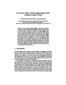
Figure 1 : Example of annotated image 2.1 Pixel color model Model This pixel color model discriminates roughly skin pixels and lip pixels. It will be used to initialize the mouth model for the first image of a sequence. We extract the CbCr values for the skin and lip pixels on our annotated training set. Then we use this set of values to calculate the distribution of a statistical variable. A Gaussian mixture model is built with the MinimumDescription-Length Algorithm to estimate this distribution. This model is appropriate for the task as it creates sub-classes able to take into count the chromatic variability between different persons. Pixels classification X contains the CbCr components of a pixel that will be classified into one of the two category Yi (with Y1: skin and Y2: lip). The probability of X to belong to one of the categories is: Ki
formula1: p ( X | Yi ) = ∑ wi , j × p ( X | ( mi , j , å j =1
i, j
))
with Ki is the number of gaussians modeling the category and wi,j, mi,j and Si,j are respectively the weight factor, the mean and the covariance matrix of each gaussian. The most likely category for the pixel is the one which maximized p(X|Yi). To take care of the pixels which belong to neither categories, we fixed a minimum threshold for p(X|Yi). This assures that the pixel is not too far from the statistical distribution. Finally either a pixel is assigned to one of the categories, either it stays unassigned. 2.2 Mouth corners local model �
�
�
�
the 3 filters (mean, horizontal and vertical gradients) and the 3 YCbCr components. So for each image of the training set we learn the responses of the filters for each mouth corners in 36 components vectors ( 3 (filters) x 3 (YCbCr component) x 4 (regions) ). The scale of the convolutions is determined by the size of the face region. The statistical distribution of these vectors will again be described by two different gaussian mixture models. The first model will test if a pixel belong to one of the two following categories: right mouth corners or left mouth corner. If Z contains the local descriptors of a pixel, the probability of this pixel to belong to one of the two category Ci (with C1: right mouth corner and C2: left mouth corner) will be p(Z|Ci) (cf formula1). The second model will test if a couple of pixel is a couple of mouth corners (so it is built with 36x2=72 components vector). It will improve the robustness by guaranteeing the coherence between the mouth corners. If V contains the local descriptors of a couple of pixels, the probability of this couple to be a couple of mouth corner will be p(V) (similar to formula1 but with only one category). 2.3 Active mouth model In this paper, we make a distinction between static appearance and dynamic appearance. Static appearance will be estimated for each speaker as the mean of the appearance : it corresponds to a generic appearance characteristic of a speaker (mouth and skin color typically). Dynamic appearance is defined as the difference between appearance and static appearance : it corresponds to the appearance variation induced by speech and movement (apparition of teeth, wrinkles or shadows for example). So extrinsic and intrinsic appearance variability are decoupled. Shape variability could have been decoupled too, but as it did not bring any significant improvement in term of goodness of segmentation this approach was not deepened. Model As the shape is already saved is the vectors si, the next step is to learn the sampled-appearance for every image. The three YCbCr components are extracted at 728 features-points given by a mesh computed from the si (as shown in figure 3). Using such a mesh will define precisely if an appearance sample corresponds to skin, lips, teeth or inner mouth. Feature-points coordinates are saved in 1456 (728x2) values vector αs,i, dynamic appearance YCbCr values in 2184 (728x3) values vector αa,i and static appearance YCbCr values in 2184 values vector ba,i (1 ≤ i ≤ N).
Figure 2 : Mouth corners area with characteristics regions, edge direction and line of luminance minima Mouth corners points will be used as key-points to determine the position and scale of the mouth. But these points are quite difficult to detect as they are often not on an edge but in shadowy region as shown in figure 2. Mouth corners will then be considered as the intersection point between 4 regions. Region 1 and 2 are non-homogeneous as they are characterized by an edge between lips and skin while on the other hand, region 3 and 4 are homogeneous on a chromatic point of view (figure 2). Mouth corners will then be described by a set of 4 local descriptors, one for each region. We chose to use gaussian derivative filters [7] for this task. We limit the model to the first gaussian derivatives and we compute the convolutions between
Figure 3: Mesh used for the sampling of appearance. Plain circles: control-points, empty circles: mesh We then proceed to a PCA as in [4] with the αs,i, αa,i and ba,i. The mean vectors ( αx s, α a, b a), the covariance matrices (Ss, Sa, Ra), their respective eigenvectors (ps,m, pa,n, qn) and eigenvalues (λs,m, λa,n, nn) with 1 ≤ m ≤ 1456 and 1 ≤ n ≤ 2184) are then calculated. For example for shape:
as =
1 N
N
∑a i =1
s ,i
; Ss =
1 N
N
∑ (a i =1
s ,i
)(
- as as ,i - as
)
T
The eigenvectors of the covariance matrices correspond
to the various variation modes of the data. As the eigenvectors with large eigenvalues describe the most significant part of the variance, the selection of a few modes can reduce the dimensionality of the problem. We chose to keep 95% of the variance in all cases. The selected eigenvectors are saved in matrices Ps, Pa and Qa. We then compute for each image the values of weight-vectors bs,i and ba,i (1 ≤ i ≤ N).
(
)
(
b s ,i = PsT as ,i - as ; b a ,i = PaT aa ,i - aa
)
We then proceed to a new PCA (as in [4]) with the values of these weight parameters to have a statistical model which links shape variation (represented by the bs,i) and dynamic appearance variability (represented by the ba,i) in order to have a coherent modelization between the two informations. We need to normalize the units difference but we also enhance shape weight over dynamic appearance which is considered to be highly related to shape and movement. This is done by the balancing coefficient W. α c is the mean vector, Sc is the covariance matrix and Pc is a matrix containing the eigenvectors to keep 95% of the variance (9 modes with eigenvalues λk, 1 ≤ k ≤ 9). T W .b s ,i 1 N W .b s ,i 1 N W .b s ,i ac = ∑ , Sc = ∑ - ac - ac N i =1 b a ,i N i =1 b a ,i b a ,i Finally we can generate any shape and sampled-appearance of the training set or new plausible examples by simply adjusting bc and da with the following equations:
as = as + Ps b s W .b s ac = = ac + Pc b c ⇒ b a aa = aa + Pa b a ba = ba + Q a d a
Segmenting mouth on an image will then consist in finding the best set of 18 parameters ( 9 in bc and 9 in da ) that control our active mouth model. To achieve this task, we define a global cost function to be minimized Cc=Cv/Cg which combines a shape criterion Cg and an appearance criterion Cv which are defined below. We also calculated the means of bc parameters vectors for each 4 GMS and we saved them in vectors bc,j (1 ≤ j ≤ 4). Mouth shape-criterion The 30 control-points which describe the lips and the teeth can be divided in 6 curves (see figure 1). If the flow of a gradient vector through these curves is maximized, then the curves will fit with the edges of the image. If G is a gradient field and ζ is a curve, the flow of vector G through ζ is calculated as: φ=
∫ G.dn ζ
∫ ds ζ
Various gradient fields are used according to the curves. Eveno [3] introduced the hybrid edge, a gradient field which combined normalized pseudo-hue with normalized luminance to enhance top frontier of the upper lip contour. In this paper we use a similar hybrid gradient field Grl by replacing pseudo-hue by Cr component: Grl ( x, y ) = -∇ [Cr ( x, y ) + L( x, y ) ]
The other gradient fields used are Gr and Gl respectively based on Cr component and luminance. For curve 1, Grl will be used to compute the flow. Gr is used for curves 2, 3 and 4 and Gl for curves 5 and 6. The gradient-based criterion Cg is computed as the sum of these 6 flows. It will be our shape criterion.
Mouth appearance-criterion This criterion Cv simply compares the YCbCr values of the sampled appearance given by the model for a set of weight parameters (bc, da) to the YCbCr values withheld in the current processed image by computing the mean square error. 3. METHOD OF SEGMENTATION 3.1 Localization of mouth corners As Eveno [3] proposed, the mouth corners are supposed to be on the line which links luminance minima for each column (see figure 2). So, we only have to find the index of the columns to know these mouth corners points. We compute the local descriptors and p(Z|Ci) for each pixel of the line of interest. We select the three pixels that have the higher probability to be a right mouth corner and the same thing for the left corner. Finally we compute p(V) for each of the 9 possible couples. The higher value of p(V) gives the mouth corners. 3.2 Lip segmentation We want to find the set of parameters for our model to obtain the best segmentation of mouth. C(In)(bc,da) is the value of a criterion for the processed image In and for the PCA parameters vectors bc and da. To minimize our cost function, we have to solve a high dimension problems. To achieve this, we use a Downhill Simplex Method (DSM), which is a minimization/maximization classical method. To run the DSM, we have to define an initial guess and a search interval for the parameters. Classically, a DSM would be initialized on the mean parameters values and the search interval would be three time the standard deviation of the modes of our active model ( 3√λk and 3√nk). To reduce the number of iterations and to increase the robustness and the accuracy of the convergence, we will try to optimize these choices. First image We use our pixel classification to broadly detect skin and lip pixels on the first image I1 and to begin to registrate the speaker.
Figure 4 : Example of pixel classification and illustration of the appearance initialization We will use this classification to find a good initial guess for da. To do so we compute the mean values of the CbCr components of the classified pixels to obtain an idea of the characteristic lip and skin color of the speaker. As luminance is not uniform on the face, we compute four mean values of Y, one for each quarter of the image (this is illustrated by figure 4). From this, we obtain a good initial set of parameters d0 representative of the chromatic characteristics of the speaker and of the general luminance of the scene. To have an initial guess of bc, we test the general mouth state (GMS) by computing the Cv(I1)(bc,j,d0) for 1 ≤ j ≤ 4, the minimum giving the initial guess (bc,j_min,d0). Then we proceed to the minimization of Cc(I1)(bc,da) by DSM and we find a final set of parameters (b1,d1). Tracking For image In+1, we check if: Cv ( In + 1)(bn, dn ) − Cv ( In )(bn, dn ) ≤ 20% Cv ( In )(bn, dn )
If this is verified, we assume that the mouth in the new image has practically the same shape that on the previous image. We will then minimize Cv(In+1)(bc,da) by DSM, with bn as initial guess and reduced search intervals 0,5√λk for parameters contained in bc. If the condition is not verified we test again the GMS to have a new initial guess and the search intervals are 3√λk. For vector parameter da, the initial guess will be the mean of all the prior dm, this mean being balanced by the corresponding final values Cv(bm,dm) (1 ≤ m ≤ n). The search interval for each parameter will be 3√nk/(1+n). If Cv(In+1)(bn+1,dn+1) > 2Cv(In)(bn,dn), we suppose the model is divergent. It can be caused by a change of lightening for example. The next image will then be computed as a first image. The DSM usually converges in 40 to 60 iterations and stops when the difference between the maximum and the minimum of the simplex is lower than a threshold value.
equal to mean error + 2*standard deviation (statistically 95% of the cases) in each direction. The model based approach blankens the error distribution that is aqually distributed on the contour. method
a
b
c
d
e
error: mean/std %
9.5/ 1.9
6/ 1.6
4.9/ 1.5
3.5/ 1.4
2.6/ 1.3
Table 2 : Successive method improvements
with a : previous method, b : new corners detector added, c : distinction between static and dynamic appearance added, d : initial pixel classification added, e : GMS added (final method)
Table 2 shows the successive improvement in robustness and accuracy brought by every new processing in our work. The “previous method” is the method of our previous paper [6] directly adapted to a multi-speaker task. Type of test images
images in training set
speaker in, images out
leave-one-out
error: mean/std %
2.63/ 1.33
2.69/ 1.36
2.81/ 1.43
Table 3 : Errors for various test protocol
Finally Table 3 shows results with different protocols and computed images in or out the training set. “Speaker in, images out” means some images of the speaker are in the training set but the computed images are not. “Leave-one-out” means the tested speaker has been totally removed from the training set.
Figure 7 : Examples of mouths rendering Figure 5 : Examples of mouths segmentation 4. RESULTS AND CONCLUSION Our method gives accurate and robust lip segmentation with precise contour detection. The initialization step gives a good clue of the chromaticity and luminance of the processed image. It improves accuracy and the speed of the convergence. Separating static and dynamic appearance allows to progressively adapt the general model to the speaker. It increases speed but also robustness as the model would react quicker to an abrupt shape change (caused by a sudden emotion, like surprise for example) as the appearance will be already well-known. The GMS increases also the robustness as the model can react to shape changes by selecting a better initial guess. 2D error position
corner lips
outer lip contour
inner lip contour
teeth
all points
error: mean/std %
3.1/ 1.4
2.6/ 1.3
2.4/ 1.3
3/ 1.4
2.6/ 1.3
Table 1 : Mean error localization. Table 1 shows the 2D mean errors and standard deviation for the shape points between detected and annotated points when the method runs on the images of the training set. These mean errors are given in percentage: the difference between detected points and annotated point is normalized by the width of the mouth.
Figure 6 : Uncertainty illustration Figure 6 gives an illustration of these errors for each position (green : corners, withe : outer contour, yellow : inner contour, red : teeth), the ellipses symbolizes the uncertainty: their radius are
In the near future a subjective evaluation is planned out that will quantify the effective enhancement in comprehension brought by the analysis-resynthesis scheme in a telephone enquiry task. Indeed, when the values of parameters are known, the sampled appearance can be interpolated by a triangle-based interpolation method. This appearance reconstruction gives a convincing and realistic clone of the speaker which seems to be quite understandable by a human lip-reader. 5. REFERENCES [1] P. Delmas, N.Eveno, and M. Lievin, “Towards Robust Lip Tracking”, International Conference on Pattern Recognition (ICPR’02),Québec City, Canada, August 2002 [2] M. Hennecke, V. Prasad, and D. Stork. “Using deformable templates to infer visual speech dynamics”, 28 h Annual Asimolar Conference on Signals, Systems, and Computer, volume 2, IEEE Computer, Pacific Grove, pages 576-582, 1994. [3] N.Eveno, A. Caplier, and P-Y Coulon, “Automatic and Accurate Lip Tracking”, IEEE Transactions on Circuits and Systems for Video Technology, vol. 14, no.5, pp. 706-715, May 2004 [4] T. F. Cootes. “Statistical models of appearance for computer vision”, Online technical report available from http: //www.isbe.man.ac.uk/bim/refs.html, 2001. [5] J. Luettin, N.A. Thacker, S.W. Beet, “Locating and Tracking Facial Speech Features”, Proceedings of the International Conference on Pattern Recognition, Vienna, Austria, 1996. [6] P. Gacon, P.-Y. Coulon, G. Bailly. “Shape and SampledAppearance model for Mouth Components Segmentation”, 5th international Workshop on Image Analysis for Multimedia Interactive Services (WIAMIS’04), Lisbon, Portugal, 2004. [7] T. Lindeberg, “Feature detection with automatic scale detection”, IJVC, vol. 30, no.2, pp. 77-116, 1998.