Applied Statictics and Operation Research Computer Modelling and New Technologies, 2010, Vol.14, No.4, 31–39 Transport and Telecommunication Institute, Lomonosova 1, LV-1019, Riga, Latvia
STATISTICAL INFERENCE USING ENTROPY BASED EMPIRICAL LIKELIHOOD STATISTICS G. Gurevich1*, A. Vexler2 1
The Department of Industrial Engineering and Management, SCE- Shamoon College of Engineering Beer-Sheva 84100, Israel E-mail:
[email protected] 2 Department of Biostatistics, The State University of New York at Buffalo Buffalo, NY 14214, USA E-mail:
[email protected]
In this article, we show that well known entropy-based tests are a product of empirical likelihood ratio. This approach yields stable definitions of entropy-based statistics for goodness-of fit tests and provides a simple development of two-sample tests based on samples entropy that have not been presented in the literature. We introduce the distribution-free density-based likelihood techniques, applied to test for goodness-of-fit. In addition, we propose and examine nonparametric two-sample likelihood ratio tests for the case-control study based on samples entropy. The Monte Carlo simulation study indicates that the proposed tests compare favourably with the standard procedures, for a wide range of null/alternative distributions. Keywords: empirical likelihood, entropy, goodness-of-fit tests, two-sample nonparametric tests, case-control study
1. Introduction The likelihood approach is a powerful and widely-used tool for parametric statistical inference. As an example, consider the simple hypothesis testing problem where given a sample of k independent identically distributed observations X 1 ,..., X k , we want to test the hypothesis
H 0 : X1 ,..., X k ~ F0 versus H 1 : X1 ,..., X k ~ F1 ,
(1)
where F0 and F1 are some distributions with density functions f 0 (x ) and f1 ( x ) , respectively. By virtue of the Neyman–Pearson Lemma, the most powerful test-statistic for (1) is the likelihood ratio k
∏ f1 ( X i ) i =1 k
∏ f 0 (X i )
,
(2)
i =1
where density functions f 0 (x ) and f1 (x ) are assumed to be completely known. However, if the alternative distribution F1 is not known, the hypotheses (1) define a goodness-of-fit problem. For this situation, to use the likelihood ratio statistic one need to estimate a likelihood function in numerator of (2). There has been much recent development of various empirical likelihood type approximations to parametric likelihood functions. The empirical likelihood (EL) method based on empirical distributions has been k
dealt with extensively in the literature (e.g., Owen [7]). The EL function has the form of L p = ∏ pi , i =1
where the components pi , i = 1,..., k maximize the likelihood L p , satisfying empirical constraints * Address for correspondence: Gregory Gurevich, The Department of Industrial Engineering and Management, SCE – Shamoon College of Engineering, Beer-Sheva 84100, Israel; e-mail:
[email protected].
31
Applied Statictics and Operation Research (e.g.,
k
k
i =1
i =1
∑ pi = 1 and ∑ pi X i = 0 ). Computation of
pi , i = 1,..., k is based on a simple exercise in Lagrange
multipliers (for details, see Owen [7]). This nonparametric approach is a result of consideration of k
the ‘distribution functions’-based likelihood
∏ (F ( X i ) − F ( X i − ))
over all distribution functions F .
i =1
Taking into account that the Neyman–Pearson Lemma operates under ‘density functions’-based forms of likelihood functions, Vexler and Gurevich [11] applied the main idea of the EL technique k
to construct density-based empirical estimation of the parametric likelihood L f = ∏ f ( X i ) , where i =1
f ( x ) is a density function. They considered the likelihood function L f in the form of L f = ∏ f ( X i ) = ∏ f (X (i ) ) = ∏ f i , where f i = f ( X (i ) ) , and X (1) ≤ X ( 2 ) ≤ … ≤ X ( k ) are the k
k
k
i =1
i =1
i =1
order statistics derived from X 1 , … , X k . The estimators of f i , i = 1, … , k that maximize L f and
((
))
satisfy some empirical constrains have the following form: f i = 2m / k X (i + m ) − X (i − m ) , i = 1, … , k .
Therefore, the maximum EL method applied to (2) with known f 0 (x ) and unknown f1 ( x ) forms the test-statistic k
Tmk =
∏ k (X i =1
2m (i + m ) − X (i − m ) )
.
k
∏ f0 (X i )
(3)
i =1
Note
⎛ k ⎞ log⎜⎜ ∏ 2m / (k (X (i + m ) − X (i −m ) ))⎟⎟ = −kH (m, k ) , ⎝ i =1 ⎠
that
where
H (m, k ) = k −1 ∑ log(k (X (i + m ) − X (i −m ) )/ 2m ) was presented by Vasicek [10], as an estimator of k
i =1
the entropy of the density
f ( x ) , for some m < k / 2 , i.e., the statistic H (m, k ) estimates
+∞
1 ⎞ ⎛ d H ( f ) = E (− log( f ( X 1 ))) = − ∫ f (x ) log( f ( x ))dx = ∫ log⎜⎜ F −1 ( p )⎟⎟dp . The power of the tests based ⎠ ⎝ dp −∞ 0 on the statistic Tmk strongly depends on values of m and this restricts applicability of (3)-type
test-statistics to real-data problems. Dealing with this problem and reconsidering their empirical constraints for density functions, Vexler and Gurevich [11] proposed the statistic k ⎛ k ⎞ 2m * Tk = min1−δ ⎜ ∏ / ∏ f 0 ( X i )⎟ as a modification of the entropy based statistic Tmk . ⎟ 1≤ m< k ⎜ i =1 k (X (i + m ) − X (i − m ) ) i =1 ⎝ ⎠ Considering the problem (1) where, under the alternative hypothesis, f1 ( x) is completely unknown, whereas, under the null hypothesis, f 0 ( x ) = f 0 (x; θ ) is known up to the vector of parameters θ = (θ1 ,...,θ d ) (here, d ≥ 1 defines a dimension of the vector θ ), they proposed the statistic
k
Gk = min1−δ 1≤ m< k
∏ k (X i =1
k
∏ i =1
2m ( i + m ) − X (i − m ) )
(
f 0 X i , θˆ
)
,
(4)
where 0 < δ < 1 and θˆ estimates θ (e.g., θˆ is the maximum likelihood estimator of θ ). They also proved that if some general conditions are satisfied for density functions f 0 ( x) , f1 ( x) and
32
Applied Statictics and Operation Research for
the
estimator
θˆ ,
then
H0 ,
under
P k −1 log(Gk ) ⎯⎯→ 0,
while,
under
H1 ,
⎛ f (X ) ⎞ P k −1 log(Gk ) ⎯⎯→ E log⎜⎜ 1 1 ⎟⎟ > 0 , where a = (a1 ,..., ad ) is a vector with finite components, as ⎝ f 0 ( X 1; a) ⎠ k → ∞ . That is, with a test-threshold C related to the type I error α = sup PH 0 (log(Gk ) > C ) in mind, θ
PH1 (log(Gk ) > C ) ⎯n⎯ ⎯→1 . That means that a test based on the statistic Gk has the asymptotic power →∞ one, i.e., is a consistent test.
2. Empirical Likelihood Ratio Tests for Uniformity and Normality 2.1. Test for Uniformity Consider a problem (1), where F0 = Unif (0,1) , F1 is an unknown distribution with a finite variance and continuous density function f1 ( x) concentrated on the interval [0,1]. In accordance with (4), the suggested test is: reject H 0 if k
min1−δ ∏
1≤ m< k
i =1
2m >C, k (X (i + m ) − X (i − m ) )
(5)
where 0 < δ < 1 , C is a test-threshold. Note that the statistic U mk =
k
∏ k (X i =1
2m with a fixed m < n / 2 was considered by (i + m ) − X (i − m ) )
Dudewicz and van der Meulen [4] as a test-statistic of the entropy-based test for uniformity. This test is a very efficient decision rule provided that optimal values of m , subject to f1 ( x) and k , are applied to the statistic U mk (Dudewicz and van der Meulen [4]). In practice, since f1 ( x) is completely unknown, we risk choosing m that leads to a U mk -based test having the power that is lower than that of other known tests for uniformity (e.g., Zhang [12]). In contrast to this, a Monte Carlo study, presented by Vexler and Gurevich [11], demonstrates that, in many cases, the test (5) provides the power that is close to the power of U mk -based tests with optimal m 's, calculated empirically. Test-threshold C for the test (5) can be obtained exactly or approximately by simulations from
⎧
⎛
⎩
⎝ 1≤m C ⎬ = α ,
for each desired
significance level α . In accordance with the asymptotic properties of the statistic (4), presented in Section 1, the test (5) is consistent as k → ∞ . 2.2. Test for Composite Hypothesis of Normality Consider a problem (1), where F0 is a normal distribution with unknown expectation μ and
(
)
variance σ 2 , F0 = Norm μ , σ 2 , F1 is an unknown distribution with a finite variance and continuous density function f1 ( x) . In accordance with (4), the suggested test is: reject H 0 if
(
min1−δ 2πes 2
1≤ m < k
) ∏ k (X ( k/2
k
i =1
2m >C, i + m ) − X (i − m ) )
(6)
2
⎞ 1 k ⎛ 1 k where 0 < δ < 1 , s = ∑ ⎜⎜ X j − ∑ X k ⎟⎟ , C is a test-threshold. k j =1 ⎝ k k =1 ⎠ 2
33
Applied Statictics and Operation Research
(
Note that the statistic N mk = 2πes 2
) ∏ (2m / k (X ( k
k/2
i+m )
i =1
− X (i −m ) )) is known, for m < n / 2 , to
be an efficient test statistic based on sample entropy (e.g., Vasicek [10], Arizono and Ohta [1]; Park and Park [8]). The tests for normality based on sample entropy are exponential rate optimal procedures (Tusnady [9]). This agrees with the fact that commonly likelihood ratio tests have optimal statistical properties and likelihood ratio type decision rules are simple in applications. The power of the test based on statistic N mk strongly depends on values of m . Assuming information regarding the distribution functions of the alternative hypothesis, Monte Carlo simulation results, published in the relevant literature, point out values of m (subject to k ) that provide high levels of the power of the test based on N mk . However, since f1 ( x) is completely unknown, we risk choosing m that leads to a N mk -based test having the power that is lower than that of other known tests for normality (e.g., Vexler and Gurevich [11]). In this sense, the main advantage of the proposed test (6) for normality is that his statistic is not depend on unknown parameters (following Vexler and Gurevich [11], we recommend the value of δ = 0.5 in definition of (6)). Since, under H 0 , the statistic of the proposed test (6) does not depend on values of μ and σ 2 , the test-threshold C for this test can be obtained exactly or approximately by simulations from
⎧
⎛
⎩
⎝ 1≤m< k
(
the equation PX1 ,…, X k ~ Norm ( 0,1) ⎨log⎜⎜ min1−δ 2πes 2
) ∏ (2m / k (X ( k/2
k
i+m)
i =1
⎫ ⎞ − X (i − m ) ))⎟⎟ > C ⎬ = α , for each ⎠ ⎭
desired significance level α . In accordance with the asymptotic properties of the statistic (4), presented in Section 1, the test (6) is consistent as k → ∞ .
3. The Proposed Two-Sample Empirical Likelihood Ratio Test for the Case-Control Study In this section, we consider independent samples of sizes n and k from two populations. The data-points in each sample are independent and identically distributed. Let X 1 ,..., X n present a control sample from distribution FX with a density function f X (x ) , and Y1 ,..., Yk be a case sample from distribution FY with a density function f Y ( y ) . We want to test the null hypothesis
H 0 : FY = FX = F0 versus H 1 : FY ≠ FX = F0 ,
(7)
where distributions F0 = FX and FY are completely unknown. In the context of (7), the likelihood ratio test statistic is n
k
i =1 n
i =1 k
i =1
i =1
∏ f X ( X i )∏ f Y (Yi ) ∏ f X ( X i )∏ f X (Yi )
= ∏ h(Yi ) = ∏ h(Y(i ) ) = ∏ hi ,
( )
k
k
k
i =1
i =1
i =1
( )
(8)
( )
where hi = h Y(i ) = f Y Y(i ) / f X Y(i ) , and Y(1) ≤ Y( 2) ≤ … ≤ Y( k ) are the order statistics based on the observations Y1 ,…, Yk . (One can present f Y = f X h , where h = f Y / f X , and hence h can be considered as an unknown function under H 1 .) Following the maximum EL methodology presented by Vexler and Gurevich [11], we find that values of hi , i = 1, … , k that maximize (8), satisfying some empirical
constraints
(( (
caused
)
(
h j = 2m / k FXn Y( j + m ) − FXn Y( j −m )
by
))) ,
the
equation
+∞
+∞
−∞
−∞
∫ f Y (u )du = ∫ f X (u )h(u )du = 1
are
n
j = 1,..., k , where FXn (x ) = n −1 ∑ I ( X i ≤ x ) is the empirical i =1
distribution function ( I (⋅) is the indicator function). Here Y( j ) = Y(1) , if j ≤ 1 , and Y( j ) = Y(k ) ,
34
Applied Statictics and Operation Research
j ≥ k . Therefore, the maximum EL method yields the entropy-based test-statistic
if
∏ [2m / k (FXn (Y( j +m ) ) − FXn (Y( j −m ) ))]. Finally, utilizing arguments of Section 1, we suggest the test-statistic k
j =1
k
2m , 0 < δ C , where
C
(10)
is
a
test-threshold.
(Similarly
FXn (x ) − FXn ( y ) = 1 / (n + k ) , if FXn ( x ) = FXn ( y ) .)
to
Canner
[3],
we
will
arbitrarily
define
Significance level of the proposed test. Since I ( X > Y ) = I (F0 ( X ) > F0 (Y )) , where F0 (x ) is the cumulative distribution function of the distribution F0 , the significance level of the test (10) is
PH 0 {log(Vnk ) > C} = PX1 ,…, X n ,Y1 ,...,Yk ~Unif ( 0,1) {log(Vnk ) > C} . That is, the type I error of the proposed
test (10) can be calculated exactly or approximately by simulations, for all sample sizes n, k and 0 < δ < 1 . Fix δ = 0.5 in (9). Table 1 displays Monte Carlo roots C of the equations PX1 ,…, X n ,Y1 ,...,Yk ~Unif ( 0,1) {log(Vnk ) > C} = α , for different values of α and n , k . For each value of α ,
n , k , the type I error results were derived via 55,000 generations of statistic log(Vnk ) 's values.
Table 1. Critical values C for the test (10) with
δ = 0.5 k
n
10
15
20
25
30
35
40
50
60
80
100
α
10
0.01 0.025 0.05 0.1
9.704 8.318 7.507 6.526
10.482 9.384 8.468 7.592
11.797 10.683 9.560 8.619
13.213 11.981 11.000 9.881
14.751 13.483 12.384 11.285
16.459 15.243 13.857 12.640
18.255 16.868 15.770 14.384
22.167 20.663 19.500 17.996
26.409 24.848 23.462 22.075
35.735 34.113 32.439 30.530
45.594 43.889 42.503 40.480
15
0.01 0.025 0.05 0.1
10.131 8.935 8.060 7.038
11.155 9.992 9.181 8.062
12.306 11.199 10.190 9.128
13.438 12.221 11.240 10.090
14.805 13.483 12.503 11.222
16.196 14.813 13.609 12.316
17.623 16.186 15.024 13.698
20.853 19.201 17.915 16.429
24.257 22.465 21.038 19.546
31.870 30.024 28.466 26.738
40.314 38.437 36.773 34.853
20
0.01 0.025 0.05 0.1
10.397 9.246 8.266 7.148
11.694 10.456 9.427 8.228
12.934 11.666 10.676 9.468
14.083 12.731 11.619 10.402
15.261 13.939 12.796 11.519
16.2465 14.899 13.723 12.430
17.526 16.086 14.923 13.565
20.188 18.683 17.382 15.841
23.094 21.420 19.980 18.328
29.707 27.898 26.306 24.390
37.090 35.069 33.337 31.309
25
0.01 0.025 0.05 0.1
10.589 9.335 8.254 7.107
12.039 10.688 9.489 8.203
13.271 11.922 10.773 9.464
14.438 12.934 11.764 10.413
15.699 14.246 13.014 11.630
16.545 15.052 13.814 12.414
17.834 16.357 15.085 13.593
20.205 18.592 17.202 15.564
22.610 20.971 19.481 17.746
28.471 26.419 24.802 22.897
34.975 32.922 30.998 28.919
30
0.01 0.025 0.05 0.1
10.645 9.380 8.263 7.083
11.884 10.466 9.363 8.083
13.374 11.881 10.715 9.375
14.542 13.001 11.730 10.265
15.846 14.284 12.961 11.458
16.928 15.274 13.883 12.326
18.120 16.447 15.059 13.443
20.260 18.603 17.119 15.427
22.485 20.719 19.117 17.356
27.820 25.810 24.010 21.960
33.479 31.332 29.433 27.133
35
0.01 0.025 0.05 0.1
10.594 9.196 8.100 6.953
11.915 10.373 9.248 7.909
13.306 11.789 10.494 9.154
14.345 12.748 11.453 9.980
15.826 14.067 12.701 11.178
16.731 15.096 13.575 11.973
18.091 16.331 14.820 13.149
20.194 18.459 16.819 15.045
22.413 20.483 18.792 16.848
27.187 25.140 23.285 21.132
32.425 30.123 28.161 25.794
35
Applied Statictics and Operation Research k
n
10
15
20
25
30
35
40
50
60
80
100
α
40
0.01 0.025 0.05 0.1
10.542 9.140 8.057 6.880
11.692 10.174 9.032 7.782
13.143 11.649 10.367 8.994
14.378 12.633 11.253 9.798
15.653 13.933 12.447 10.882
16.659 14.749 13.211 11.606
17.875 16.116 14.537 12.742
20.127 18.112 16.407 14.490
22.212 20.171 18.316 16.272
26.927 24.653 22.679 20.312
31.777 29.379 27.324 24.705
50
0.01 0.025 0.05 0.1
10.250 8.924 7.823 6.678
11.548 9.997 8.802 7.607
12.860 11.241 9.967 8.655
13.744 12.013 10.709 9.367
15.137 13.282 11.874 10.325
15.875 14.045 12.540 11.015
17.343 15.403 13.754 12.045
19.466 17.286 15.482 13.571
21.533 19.242 17.281 15.204
26.053 23.424 21.223 18.738
30.349 27.738 25.326 22.406
60
0.01 0.025 0.05 0.1
10.312 8.861 7.737 6.624
11.157 9.745 8.660 7.466
12.501 10.894 9.669 8.405
13.428 11.757 10.411 9.092
14.524 12.784 11.371 9.988
15.238 13.448 12.019 10.577
16.559 14.664 13.112 11.486
18.439 16.261 14.562 12.843
20.254 17.972 16.207 14.318
24.498 21.796 19.684 17.395
28.806 25.743 23.256 20.587
80
0.01 0.025 0.05 0.1
9.989 8.620 7.576 6.494
10.851 9.457 8.356 7.199
11.833 10.409 9.268 8.037
12.642 11.126 9.893 8.665
13.838 12.134 10.815 9.506
14.275 12.685 11.366 9.980
15.393 13.677 12.231 10.796
17.002 15.043 13.597 12.037
18.684 16.575 14.948 13.238
21.884 19.583 17.708 15.767
25.703 22.919 20.792 18.479
100
0.01 0.025 0.05 0.1
9.824 8.499 7.512 6.448
10.569 9.221 8.190 7.085
11.567 10.187 9.091 7.892
12.218 10.724 9.597 8.446
13.171 11.621 10.469 9.205
13.806 12.262 10.989 9.692
14.709 13.017 11.712 10.349
16.179 14.324 12.919 11.486
17.356 15.537 14.087 12.549
20.413 18.149 16.540 14.866
23.243 21.008 19.067 17.043
0.01 0.025 0.05 0.1
9.138 7.967 7.029 6.080
9.623 8.486 7.579 6.626
10.291 9.081 8.157 7.182
10.650 9.493 8.555 7.581
11.113 9.930 9.017 8.025
11.449 10.271 9.343 8.360
11.888 10.689 9.722 8.722
12.507 11.311 10.363 9.357
13.125 11.891 10.937 9.920
14.232 12.993 12.004 10.957
15.225 13.955 12.933 11.850
∞
The following propositions present asymptotic operating characteristics of the test (10). Proposition 3.1. For each 0 < δ < 1 , k
2m , as n → ∞ , j =1 k Z ( j + m ) − Z ( j − m )
P Vnk ⎯⎯→ min1−δ ∏ 1≤ m < k
(
)
where under H 0 , Z 1 ,..., Z k ~ Unif (0,1) , whereas under H 1 , Z1 ,..., Z k ~ FZ , and FZ is a nonuniform distribution function with a density function f Z concentrated on [0,1]. Proof. We note that, for each 1 ≤ i ≤ k and ε > 0 , we have
P ( FXn (Yi ) − FX (Yi ) > ε ) =
+∞
∫ P( FXn ( y ) − FX ( y ) > ε ) f Y ( y )dy ⎯n⎯→⎯∞ → 0 .
−∞
⎯→ FX (Yi ) = Z i , as n → ∞ . Obviously, under H 0 , Z i has the uniform Therefore, FXn (Yi ) ⎯ P
Unif (0,1) distribution. Under H 1 , the distribution of the Z i is not uniform but concentrated on the interval [0,1]. When the control-sample size n → ∞ , the rule (10) rejects H 0 if
⎛ k 2m min1−δ log⎜ ∏ ⎜ j =1 k Z ( j + m ) − Z ( j −m ) 1≤ m< k ⎝
(
)
⎞ ⎟>C ⎟ ⎠
(11)
( C is from (10)). Note that, (11) is an empirical likelihood modification of the well-known test for uniformity proposed by Dudewicz & Van Der Meulen [4]. Monte Carlo critical values C for the test (11), corresponding to different values of α and k , are presented in the last lines of the Table 1 (signed n = ∞ ). These critical values can be used for the two-sample test (10) based on data with a large number of controls X 1 ,..., X n .
36
Applied Statictics and Operation Research Proposition 3.2. For each δ ∈ (0,1) ,
⎯→ 0 , as n → ∞ , k → ∞ ; under H 0 , k −1 log(Vnk ) ⎯ P
⎯→ b , as n → ∞ , k → ∞ , under H 1 , k −1 log(Vnk ) ⎯ where b is a positive constant. P
Proof. By virtue of Proposition 3.1, for each 0 < δ < 1 , k ⎛ 2m P ⎯→ k −1 log(Vnk ) ⎯ k −1 log⎜ min1−δ ∏ ⎜ 1≤ m< k j =1 k Z ( j + m ) − Z ( j − m ) ⎝
(
)
⎞ ⎟ , as n → ∞ , ⎟ ⎠
(12)
where Z i = FX (Yi ) . Let FZ define the distribution of Z j with a density function f Z , j = 1,..., k .
We pointed out in the proof of Proposition 3.1 that under H 0 , FZ is the uniform Unif (0,1) distribution. Under H 1 , FZ is not uniform but FZ is concentrated on the interval [0,1]. Consider a behavior of
⎛
k
⎝
j =1
((
the statistic k −1 log⎜ min1−δ ∏ 2m k Z ( j + m ) − Z ( j − m ) ⎜ 1≤m< k k ⎛ 2m k −1 log⎜ min1−δ ∏ ⎜ 1≤m< k j =1 k Z ( j + m ) − Z ( j − m ) ⎝
(
where p mk = k −1
)
−1
⎟ , as k → ∞ . Note that ⎟ ⎠
⎞ ⎟ = − max p mk , ⎟ 1≤ m< n1−δ ⎠
∑ log(k (Z ( j +m ) − Z ( j −m ) )/ 2m). Following Vasicek [10], after some reorganization, k
j =1
we obtain
p mk = (2m )
−1 ⎞
))
(
)
(
)( (
⎛ FZ Z ( j + m ) − FZ Z ( j −m ) ⎞ ⎟ FZk Z ( j + m ) − FZk Z ( j − m ) , ⎟ Z − Z j =1 ( j + m ) ( j − m ) ⎝ ⎠ 1 k k ⎛ ⎞ FZ Z ( j + m ) − FZ Z ( j − m ) ⎟ , = ∑ log⎜ k j =1 ⎝ 2m ⎠
2m
k
∑ S i + U mk , S i = −∑ log⎜⎜ i =1
( (
j ≡ i(mod 2m ) , U mk
)
(
)
(
))
))
1 k ∑ I (Z i ≤ x ) are the cumulative and empirical distribution functions, k i =1 respectively. Vasicek [10] showed that S i uniformly converges in probability to the entropy of the density
where FZ ( x ) and FZk ( x ) =
f Z ( x ) (as k → ∞ , m / k → 0 ), for all 1 ≤ m ≤ k 1−δ , 0 < δ < 1 . The statistic U mk is a non-positive
⎯→ 0 as k → ∞ , m → ∞ . Thus, random variable distributed independently of FZ and U mk ⎯ P
k ⎛ 2m k −1 log⎜ min1−δ ∏ ⎜ 1≤m< k j =1 k Z ( j + m ) − Z ( j − m ) ⎝ k ⎛ 2m k −1 log⎜ min1−δ ∏ ⎜ 1≤m