arXiv:quant-ph/9810022v5 14 Feb 2000. Stochastic Phase Space Localisation for a Single Trapped Particle. Stefano Manciniâ, David Vitali and Paolo Tombesi.
Stochastic Phase Space Localisation for a Single Trapped Particle Stefano Mancini∗ , David Vitali and Paolo Tombesi Dipartimento di Matematica e Fisica, Universit` a di Camerino, via Madonna delle Carceri I-62032 Camerino and Istituto Nazionale per la Fisica della Materia, Camerino, Italy (February 1, 2008)
arXiv:quant-ph/9810022v5 14 Feb 2000
We propose a feedback scheme to control the vibrational motion of a single trapped particle based on indirect measurements of its position. It results the possibility of a motional phase space uncertainty contraction, corresponding to cool the particle close to the motional ground state.
I. INTRODUCTION
In recent years there has been an increasing interest on trapping phenomena and related cooling techniques [1]. Some years ago it has been shown that, using resolved sideband cooling, a single ion can be trapped and cooled down near to its zero-point vibrational energy state [2] and recently, analogous results have been obtained for neutral atoms in optical lattices [3]. The possibility to control trapped particles, indeed, gave rise to new models in quantum computation [4], in which information is encoded in two internal electronic states of the ions and the two lowest Fock states of a vibrational collective mode are used to transfer and manipulate quantum information between them. It may happen however, that a trapped ion that is a favorable candidate for quantum information processing since it posseses a hyperfine structure with long coherence times (as for example 25 Mg+ [5]), is not suitable for resolved sideband cooling. In such cases it may be helpful to have an alternative cooling technique, which can be applied when resolved sideband cooling is impractical to use. In this paper we present a way to control the motion of a trapped particle, which is able to give a significant phase-space-localisation. The basic idea of the scheme is to realize an effective and continuous measurement of the position of the trapped particle and then apply a feedback loop able to decrease the position fluctuations. Due to the continuous nature of the measurement and to the effect of the trapping potential coupling the particle position with its momentum, feedback will realize an effective phase-space localisation. With this respect there are some analogies between the present method and resolved-sideband stimulated Raman cooling [6], which can be viewed as a sort of feedback scheme. In fact, one of the two Raman lasers performs an effective measurement of the vibrational number by changing the particle internal state only if it is an excited vibrational state. The second Raman laser performs instead the feedback step, because it puts the particle back in the initial internal state, after having removed a vibrational quantum. The feedback scheme proposed here measures the particle position rather than its energy and tries to achieve cooling as phase-space localisation, using the particle oscillatory motion to mix position and momentum quadratures. A second analogy is given by the fact that the proposed method needs a Doppler pre-cooling stage, as it happens for resolved sideband cooling. In fact, the effective trapped particle position measurement is realized only in the Lamb-Dicke regime, i.e. when the recoil energy is much smaller than the energy of a vibrational quantum, which can be obtained only when the particle has undergone a preliminary cooling stage. Our scheme will provide therefore further phase space localisation and cooling. The paper is organized as follows. In section II we show how to realize the indirect continuous measurement of the position by coupling the trapped particle with a standing wave. In section III we shall introduce the feedback loop, in section IV we shall study the properties of the stationary state in the presence of feedback and section V is for concluding remarks.
∗
Present address: Dipartimento di Fisica, Universit` a di Milano, Via Celoria 16, I-20133 Milano, Italy.
1
II. CONTINUOUS POSITION MEASUREMENT
We consider a generic particle trapped in an effective harmonic potential. For simplicity we shall consider the one-dimensional case, even if the method can be in principle generalized to the three-dimensional case. This particle can be an ion trapped by a linear rf-trap [7] or a neutral atom in an optical trap [3,8]. Our scheme however does not depend on the specific trapping method employed and therefore we shall always refer from now on to a generic trapped “atom”. The trapped atom of mass m, oscillating with frequency ν along the x ˆ direction and with position operator x = x0 (a + a† ), x0 = (¯ h/2mν)1/2 , is coupled to a standing wave with frequency ωb , wave-vector k along xˆ and annihilation operator b. The standing wave is quasi-resonant with the transition between two internal atomic levels |+i and |−i. The Hamiltonian of the system is [9] H=
hω0 ¯ σz + h ¯ νa† a + h ¯ ωb b† b + i¯hǫ(σ+ + σ− )(b − b† ) sin (kx + φ) , 2
(1)
where σz = |+ih+| − |−ih−|,�σ± = |±ih∓|, and ǫ is the coupling constant. In the interaction representation with respect to H0 = h ¯ ω b† b + σ2z , where ω ∼ ωb will be specified later, and making the rotating wave approximation, this Hamiltonian becomes H=
¯∆ h σz + h ¯ νa† a + h ¯ δb† b + i¯hǫ(σ+ b − σ− b† ) sin (kx + φ) , 2
(2)
where ∆ = ω0 − ω and δ = ωb − ω are the atomic and field mode detuning, respectively. There are now two different ways for realizing an effective continuous measurement of the atom position and we shall describe them separately, even if they present many similarities. A. The Resonant case
We consider the case when the standing wave is perfectly resonant with the |+i ↔ |−i transition, i.e., ωb = ω0 . It is therefore convenient to choose the frequency of the rotating frame ω = ωb = ω0 in this case, so that both detunings are equal to zero. Moreover we shall consider the case of a very intense standing wave, so that it can be treated classically, that is, b can be replaced by the c-number β. Choosing the phase of the field such that β = −i|β|, Hamiltonian (2) becomes H=h ¯ νa† a + h ¯ ǫ|β|σx sin (kx + φ) ,
(3)
where σx = σ+ + σ− . If we finally set the spatial phase φ = 0 (i.e. the atom is trapped near a node of the classical standing wave) and assume the Lamb-Dicke regime, we can approximate the sine term at first order and get [10,11] H=h ¯ νa† a + h ¯ χσx X ,
(4)
where χ = 2ǫ|β|kx0 is the effective coupling constant between the internal and the vibrational degrees of freedom, and X = (a + a† )/2 is the dimensionless position operator of the trapped atom. This Hamiltonian shows how one can realize an effective measurement of the atomic position. In fact, the atom displacement away from the electric field node increases the probability of electronic excitation, and hence displacements can be monitored by means of the atomic fluorescence. Therefore, the two-level (sub)system can be used as a meter to measure the position quadrature X. The evolution equation for the total density operator D for the vibrational degree of freedom and the internal states is determined by Hamiltonian (4) and by the terms describing the spontaneous emission from the level |+i responsible for the fluorescence, Lspont D =
κ (2σ− Dσ+ − σ+ σ− D − Dσ+ σ− ) , 2
(5)
where κ is the spontaneous emission rate. Here we have neglected the recoil and the associated heating of the vibrational motion. This is reasonable in the Lamb-Dicke limit we have assumed from the beginning, since the associated heating rate is given by κ(kx0 )2 vibrational quanta per second, which is negligible for a sufficiently small Lamb-Dicke parameter kx0 . In practical situations, also other heating mechanisms exist, caused by technical imperfections such 2
as the fluctuations of trap parameters due to ambient fluctuating electrical fields in the ion trap case [7], and due to laser intensity noise and beam-pointing fluctuations in the case of far-off resonance optical traps (see Ref. [8] and references therein). We assume the presence of this heating due to trap imperfections, and we describe it with the following term in the master equation, characterized by a heating rate γh (see [12]) Lh D =
� � γh γh 2aDa† − a† aD − Da† a + 2a† Da − aa† D − Daa† . 2 2
(6)
The heating rate γh has not to be too large, in order to stay within the assumed Lamb-Dicke regime. The Lamb-Dicke condition also implies that the trapped atom has to be initially prepared in a sufficently cold state, i.e., an effective thermal state with, say, a mean vibrational number n0 ∼ 10. This can be obtained with a preliminary Doppler cooling stage, which is then turned off at t = 0 and replaced by the proposed feedback cooling scheme. We shall see that our scheme is able to further cool the trapped atom, close to the ground state, even in the presence of moderate heating processes. The resulting master equation for the internal and vibrational degrees of freedom is i κ D˙ = Lh D − [H, D] + (2σ− Dσ+ − σ+ σ− D − Dσ+ σ− ) . h ¯ 2
(7)
Let us now see how to realize the continuous position measurement. It has been recently shown that when excited by a low intensity laser field, a single trapped atom emits its fluorescent light mainly within a quasi-monochromatic elastic peak [13]. The fluorescent light spectrum was measured by heterodyne detection. By improving the technique it does not seem impractical to get a homodyne detection of the single-ion fluorescent light. In Ref. [14], it was shown how one could achieve such a measurement. �Thus, by exploiting the resonance fluorescence it could be possible to measure the quantity Σϕ = σ− e−iϕ + σ+ eiϕ through homodyne detection of the field scattered by the atom along a certain direction [9]. In fact, the detected field may be written in terms of the dipole moment operator for the transition |−i ↔ |+i as [9] √ Es(+) (t) = ηκσ− (t) , (8) where η is an overall quantum efficiency accounting for the detector efficiency and the fact that only a small fraction of the fluorescent light is collected and superimposed with a mode-matched oscillator. As a consequence of (8), the homodyne photocurrent will be [15] √ (9) I(t) = 2ηκhΣϕ (t)ic + ηκξ(t) , where the phase ϕ is related to the local oscillator, which, since we have assumed the resonance condition ∆ = 0, in the present case is provided by the same driving field generating the classical standing wave. The subscript c in Eq. (9) denotes the fact that the average is performed on the state conditioned on the results of the previous measurements and ξ(t) is a Gaussian white noise [15]. In fact, the continuous monitoring of the electronic mode performed through the homodyne measurement, modifies the time evolution of the whole system, and the state conditioned on the result of measurement, described by a stochastic conditioned density matrix Dc , evolves according to the following stochastic differential equation (considered in the Ito sense) i κ D˙ c = Lh Dc − [H, Dc ] + (2σ− Dc σ+ − σ+ σ− Dc − Dc σ+ σ− ) h ¯ 2 � √ + ηκ ξ(t) e−iϕ σ− Dc + eiϕ Dc σ+ − 2hΣϕ ic Dc .
Since we are considering a strong fluorescent transition it is reasonable to assume that the spontaneous emission rate κ is large, i.e., κ ≫ χ. This means that the internal two-level system is heavily damped and that it will almost always be in its lower state |−i. This allows us to adiabatically eliminate the internal degree of freedom and to perform a perturbative calculation in the small parameter χ/κ, obtaining (see also Ref. [16]) the following expansion for the total conditioned density matrix Dc Dc = ρc ⊗ |−ih−| − i
χ (Xρc ⊗ |+ih−| − ρc ⊗ |−ih+|X) , κ
(10)
where ρc = Trel Dc is the reduced conditioned density matrix for the vibrational motion. In the adiabatic regime, the internal dynamics instantaneously follows the vibrational one and therefore one gets information on the position dynamics X by observing the quantity Σϕ . The relationship between the conditioned mean values follows from Eq.(10) 3
hΣϕ (t)ic =
χ hX(t)ic sin ϕ . κ
(11)
Moreover, if we adopt the perturbative expression (10) for Dc in (10) and perform the trace over the internal mode, we get an equation for the reduced density matrix ρc conditioned to the result of the measurement of the observable hΣϕ (t)ic , and therefore hX(t)ic � χ2 � ρ˙ c = Lh ρc − iν a† a, ρc − [X, [X, ρc ]] 2κ p � + ηχ2 /κ ξ(t) ieiϕ ρc X − ie−iϕ Xρc + 2 sin ϕhX(t)ic ρc .
(12)
This equation describes the stochastic evolution of the vibrational state of the trapped atom conditioned to the result of the continuous homodyne measurement of the resonance fluorescence. The double commutator with X is typical of quantum non-demolition (QND) measurements of the position. However this indirect measurement is not properly QND because of the presence of the vibrational bare Hamiltonian h ¯ νa† a mixing the position quadrature with the momentum.
B. The Off-Resonant Interaction
One can realize an effective indirect measurement of the atomic position also in the opposite limit of large detuning between the standing wave field and the internal transition. In fact, when the internal detuning ∆ is very large (∆ ≫ ν, δ, κ, ǫ) the excited level |+i can be adiabatically eliminated: the state of the whole system (atom+standing wave mode) can be written as ψ+ |+i + ψ− |−i, and adding a constant term h ¯ ∆/2 to the Hamiltonian (2), the corresponding Schr¨odinger equations will be iψ˙ + = (∆ + νa† a + δb† b)ψ+ + iǫ sin(kx + φ)bψ− iψ˙ − = (νa† a + δb† b)ψ− − iǫ sin(kx + φ)b† ψ+ .
(13) (14)
In the adiabatic limit of very large ∆ we can neglect the time derivative in (13) and put ψ+ ≃ −i
ǫ sin(kx + φ)bψ− . ∆
(15)
Inserting this equation into (14), one gets an equation for ψ− which is equivalent to have the following effective Hamiltonian for the vibrational motion of the atom and the standing wave mode alone H=h ¯ δb† b + h ¯ νa† a − ¯h
ǫ2 † b b sin2 (kx + φ) . ∆
If we now set the spatial phase φ = π/4, we can rewrite (16) as � � ǫ2 ǫ2 † H =h ¯ δ− b† b + h ¯ νa† a − ¯h b b sin (2kx) . 2∆ 2∆
(16)
(17)
It is clear that in this case it is convenient to choose the frequency ω of the rotating frame so that δ = ǫ2 /2∆. The Hamiltonian (17) assumes the desired form when the Lamb-Dicke regime is again assumed so to approximate the sine term with its argument, and when the case of an intense standing wave is considered. However, in this case we shall not neglect the quantum fluctuations of the standing wave field, and we shall make the replacement b → β + b, where β ≫ 1 describes the classical coherent steady state of the radiation mode and b is now the annihilation operator describing the quantum fluctuations. One gets H=h ¯ νa† a − ¯h
ǫ2 kx(|β|2 + β ∗ b + βb† ) . ∆
(18)
Shifting the origin along the x direction by the quantity h ¯ ǫ2 k|β|2 /∆mν 2 , one finally gets an effective Hamiltonian analogous to that of the resonant case (4) H =h ¯ νa† a + h ¯ χY X , 4
(19)
where now χ = −4|β|kx0 ǫ2 /∆ and the atomic polarization σx is replaced by the standing wave field quadrature Y = (be−iφβ + b† eiφβ )/2, where φβ is the phase of the classical amplitude β. This means that in this case the “meter” is represented by the cavity mode, and that an effective continuous measurement of the position of the trapped atom is provided by the homodyne measurement of the light outgoing from the cavity. This measurement allows in fact to obtain the quantity Yϕ = (ae−iϕ + a† eiϕ )/2, which is analogous to the quantity Σϕ of the previous Section. Therefore, all the steps leading to Eq. (12) in the preceding subsection, can be repeated here, with the appropriate changes. In this non-resonant case, D now refers to the density matrix of the system composed by vibrational mode and the standing wave mode and the spontaneous emission term in the master equation (7) has to be replaced by the formally analogous term describing damping of the standing wave mode due to photon leakage. This is equivalent to interpret the parameter κ as a cavity mode decay rate in this case and to replace σ− with b, σ+ with b† , and Σϕ with Yϕ in Eqs. (7), (8), (9) and (10). It is again reasonable to assume that the standing wave mode is highly damped, i.e. κ ≫ χ, so that it is possible to eliminate it adiabatically. The perturbative expansion (10) now becomes � � χ χ2 Dc = ρc − 2 Xρc X ⊗ |0ih0| − i (Xρc ⊗ |1ih0| − ρc X ⊗ |0ih1|) κ κ � χ2 χ2 + 2 Xρc X ⊗ |1ih1| − √ X 2 ρc ⊗ |2ih0| + ρc X 2 ⊗ |0ih2| , (20) 2 κ κ 2
where |ni, n = 0, 1, 2, are the lowest standing wave mode Fock states. Using this adiabatic expansion and tracing over the standing wave mode, one finally gets exactly Eq. (12), describing the reduced dynamics of the vibrational mode conditioned to the result hX(t)ic of the continuous position measurement. III. THE FEEDBACK LOOP
We are now able to use the continuous record of the atom position to control its motion through the application of a feedback loop. We shall use the continous feedback theory proposed by Wiseman and Milburn [17]. One has to take part of the stochastic output homodyne photocurrent I(t), obtained from the continuous monitoring of the meter mode, and feed it back to the vibrational dynamics (for example as a driving term) in order to modify the evolution of the mode a. To be more specific, the presence of feedback modifies the evolution of the conditioned state ρc (t). It is reasonable to assume that the feedback effect can be described by an additional term in the master equation, linear in the photocurrent I(t), i.e. [17] [ρ˙ c (t)]f b =
I(t − τ ) Kρc (t) , ηχ
(21)
where τ is the time delay in the feedback loop and K is a Liouville superoperator describing the way in which the feedback signal acts on the system of interest. The feedback term (21) has to be considered in the Stratonovich sense, since Eq. (21) is introduced as limit of a real process, then it should be transformed in the Ito sense and added to the evolution equation (12). A successive average over the white noise ξ(t) yields the master equation for the vibrational density matrix ρ in the presence of feedback. Only in the limiting case of a feedback delay time much shorter than the characteristic time of the a mode, it is possible to obtain a Markovian equation [17,18], which is given by � � χ2 � K2 ρ˙ = Lh ρ − iν a† a, ρ − [X, [X, ρ]] + K ieiϕ ρX − ie−iϕ Xρ + ρ. 2κ 2ηχ2 /κ
(22)
The second term of the right hand side of Eq. (22) is the usual double-commutator term associated to the measurement of X; the third term is the feedback term itself and the fourth term is a diffusion-like term, which is an unavoidable consequence of the noise introduced by the feedback itself. Then, since the Liouville superoperator K can only be of Hamiltonian form [17], we choose it as Kρ = −ig [P, ρ] /2 [16], where P = (a − a† )/2i is the adimensional momentum operator of the trapped particle and g is the feedback gain related to the practical way of realizing the loop. One could have chosen to feed the system with a generic phase-dependent quadrature; however, it is possible to see that the above choice gives the best and simplest result [16]. Using the above expressions in Eq. (22) and rearranging the terms in an appropriate way, we finally get the following master equation:
5
� � Γ Γ (N + 1) 2aρa† − a† aρ − ρa† a + N 2a† ρa − aa† ρ − ρaa† 2 2 � � Γ ∗ Γ † † †2 †2 − M 2a ρa − a ρ − ρa − M 2aρa − a2 ρ − ρa2 2 2 � � � � g − sin ϕ a2 − a†2 , ρ − iν a† a, ρ , 4
ρ˙ =
where
Γ = −g sin ϕ ; � � χ2 1 g2 1 γh + − ; + N =− g sin ϕ 4κ 4ηχ2 /κ 2 � 2 � 1 i χ g2 M= − cot ϕ . − g sin ϕ 4κ 4ηχ2 /κ 2
(23)
(24) (25) (26)
Eq. (23) is very instructive because it clearly shows the effects of the feedback loop on the vibrational mode a. The proposed feedback mechanism, indeed, not only introduces a parametric driving term proportional to g sin ϕ, but it also simulates the presence of a squeezed bath [19], characterized by an effective damping constant Γ and by the coefficients M and N , which are given in terms of the feedback parameters [16]. An interesting aspect of the effective bath described by the first four terms in the right hand side of (23) is that it is characterized by phase-sensitive fluctuations, depending upon the experimentally adjustable phase ϕ. This master equation preserves the positivity of ρ provided that the condition |M |2 ≤ N (N + 1) is satisfied [19], as it can be checked in the present case. In fact, under this condition it is always possible to find a unitary transformation transforming Eq. (23) into a master equation manifestly of the Lindblad form. IV. THE STATIONARY SOLUTION
Because of its linearity, the solution of Eq. (23) can be easily obtained by using the normally ordered characteristic function [19] C(λ, λ∗ , t). The partial differential equation corresponding to Eq. (23) is � � � � � � g Γ Γ ∗ ∗ + iν λ∂λ + − iν λ ∂λ∗ + sin ϕ (λ∂λ∗ + λ ∂λ ) C(λ, λ∗ , t) ∂t + 2 2 2 � � � � � � Γ g Γ ∗ g 2 ∗ 2 = −ΓN |λ| + (27) M + sin ϕ (λ ) + M + sin ϕ λ2 C(λ, λ∗ , t) , 2 4 2 4 The stationary state is reached only if the parameters satisfy the stability condition that all the eigenvalues have positive real part, which in the present case is achieved when g sin ϕ < 0. In this case the stationary solution has the following form � � 1 1 (28) C(λ, λ∗ , ∞) = exp −ζ|λ|2 + µ(λ∗ )2 + µ∗ λ2 , 2 2 where N (g 2 sin2 ϕ + 4ν 2 ) + g sin ϕ (2νIm{M } − g sin ϕRe{M }) + g 2 sin2 ϕ/2 ; 4ν 2 (N + 1/2)g sin ϕ + ΓRe{M } + 2νIm{M } µ=Γ 4ν 2 g sin ϕ +i [Re{M } − (N + 1/2)] . 2ν ζ=
(29)
(30)
This means that in general, the stationary state is a generalized gaussian state. However, in practical situations, the stationary state assumes a much simpler form. In fact, the vibrational frequency ν is usually much larger than the heating rate γh and the feedback parameter g, and in this limit, Eqs. (29) and (30) become ζ ≈ N and µ ≈ 0 respectively. Using Eq. (28), one has � � (31) C(λ, λ∗ , ∞) = exp −N |λ|2 , 6
that is, the stationary state is an effective thermal state with mean vibrational number N . This can also be seen from the fact that in the large ν limit, one can consider the master equation (23) in the frame rotating at the frequency ν, and neglecting the rapidly oscillating terms, one ends up with a thermal master equation given by the first line of Eq. (23), whose steady state is just the thermal state with mean phonon number N . The expression for N given by Eq. (24) shows that it is convenient to choose ϕ = −π/2 to get the smallest possible values for N . In this way the stability condition is also automatically satisfied. Then, the minimum value for the stationary mean vibrational number N can be obtained by minimizing it with respect to the feedback gain g: the � �1/2 optimal value for g is given by g = 4 γh + χ2 /4κ ηχ2 /4κ and the corresponding minimum value of N is "s # 1 + 4κγh /χ2 1 −1 . (32) Nmin = 2 η This expression shows the best cooling result achievable with the present feedback scheme. One has that when the heating rate is negligible with respect to the “QND coupling” parameter χ2 /4κ, the final vibrational number N is limited only by the efficiency of the homodyne measurement η. In particular this fact is true in the optimal case where all the technical sources of heating are eliminated which means γh = 0 in all the above expressions. Therefore, the present scheme is able to achieve cooling to the motional ground state especially in the off-resonant scheme, in which the particle position measurement is realized through homodyning the radiation exiting the cavity. In fact, in this case the homodyne efficiency can be very close to one. This is shown in Fig. 1, where we have sketched the √ phase space uncertainty contours obtained by cutting the Wigner function corresponding to Eq.(28) at 1/ e times its maximum height. We see that the feedback produces a relevant contraction of the uncertainty region, which becomes almost indistinguishable from the region corresponding to the motional ground state (inner dotted line in Fig. 1). The outer dashed line corresponds instead to the initial thermal state with mean vibrational number n0 = 10, prepared by the Doppler pre-cooling stage. In the resonant case in which the effective position measurement is realized through the homodyne measurement of the fluorescence, the measurement efficiency is much lower and ground state cooling becomes very difficult to achieve. However, this position measurement scheme based on fluorescence becomes necessary when one cannot extract the light out of a cavity, such as in Ref. [13], and one has to use the fluorescent light. V. CONCLUSIONS
We have proposed a feedback scheme able to achieve significant cooling of the motional degree of freedom of a trapped particle. The method is based on an effective continuous measurement of the particle position which can be realized in two different ways: by homodyning either the fluorescence of a strong transition or directly the light exiting the cavity which is coupled to the trapped particle. When the efficiency of the homodyne detection is close to one, the method is able to achieve ground state cooling. It is interesting to note that, even if only the particle position is measured and the feedback is chosen in order to decrease position fluctuations, the scheme provides a phase-space localisation for all quadratures. This is essentially due to the fact that the bare atom Hamiltonian h ¯ νa† a mixes the dynamics of the atomic position and momentum, so that the continuous homodyne measurement actually gives informations on both quadratures. This model shares some peculiarities with that one we have proposed in [20] to cool the vibrational motion of a macroscopic mirror of an optical cavity. The present application to a trapped atom stresses the versatility of the methods using feedback loops in systems characterized by the radiation pressure force in controlling thermal noise. It is also possible to see that the proposed scheme is not able to reduce the noise below the quantum limit, i.e. the stationary state variance of a generic motional quadrature cannot be made smaller than 1/4. This is again a consequence of the free vibrational Hamiltonian h ¯ νa† a (it is in fact possible to get position squeezing in the limiting case ν = 0 [21]). Actually, position squeezing can be obtained by considering a suitable modification of the present scheme [22]. As concerns the specific way in which a particular feedback Hamiltonian could be implemented, the important point is to be able to realize a term in the feedback Hamiltonian proportional to momentum. This is not straightforward, but could be realized by using the feedback current to vary an external potential applied to the atom without altering the trapping potential. On the other hand, shifts in the position (being strictly equivalent to a linear momentum term in the Hamiltonian), are achieved simply by shifting all the position dependent terms in the Hamiltonian, in particular the trapping potential. Alternatively, the use of laser pulses could be useful as well, since, using a typical laser cooling scheme, the light can exert on the atom a force proportional to its momentum. 7
As we have already remarked, in principle the model could be extended to the three dimensional case. As concerns the model discussed in Sec. II A, one should consider three different internal transitions, each one coupled with a vibrational degree of freedom, resonant with three orthogonal standing waves. For the off-resonant case presented in Sec. II B, one should only consider three orthogonal standing waves far from resonant transitions. In conclusion, although the implementation of the presented cooling method via feedback could be an hard task, it can be useful whenever the use of resolved sideband cooling is impractical. The possibility of having an alternative way to cool trapped particles is particularly interesting for quantum information processing applications, because it may happen that the requirement of having two highly stable internal states for quantum logic operations and a good internal transition for sideband cooling cannot be simultaneously satisfied. With this respect other cooling strategies have been recently proposed, as for example the use of sympathetic cooling between two different species of ions [5,23]. ACKNOWLEDGEMENTS
This work has been partially supported by INFM (through the Advanced Research Project “CAT”), by the European Union in the framework of the TMR Network “Microlasers and Cavity QED”.
[1] see e.g., P. K. Ghosh, Ion Traps, (Clarendon, Oxford, 1995), and references therein. [2] F. Diedrich, J.C. Bergquist, W.M. Itano and D.J. Wineland, Phys. Rev. Lett. 62, 403 (1989). [3] S.E. Hamann, D.L. Haycock, G. Close, P.H. Pax, I.H. Deutsch, and P.S. Jessen, Phys. Rev. Lett. 80, 4149 (1998); M.T. DePue, C. McCormick, S.L. Winoto, S. Oliver, and D.W. Weiss, Phys. Rev. Lett. 82, 2262 (1999); S. Friebel, C. D’Andrea, J. Walz, M. Weitz, and T.W. Hansch, Phys. Rev. A 57, R20 (1998). [4] J.I. Cirac, P. Zoller, Phys. Rev. Lett. 74, 4091 (1995). [5] E. Peik, J. Abel, Th. Becker, J. von Zanthier, and H. Walther, Phys. Rev. A 60, 439 (1999). [6] C. Monroe, D.M. Meekhof, B.E. King, S.R. Jefferts, W.M. Itano, D.J. Wineland, and P. Gould, Phys. Rev. Lett. 75, 4011 (1995). [7] D.J. Wineland, C. Monroe, W.M. Itano, D. Leibfried, B.E. King, D.M. Meekhof, J. Res. Natl. Inst. Stand. Technol. 103, 259 (1998). [8] T.A. Savard, K.M. O’Hara, and J.E. Thomas, Phys. Rev. A 56, R1095 (1997). [9] see e.g., D. F. Walls and G. J. Milburn, Quantum Optics, (Springer, Berlin, 1994). [10] C.A. Blockley, D. F. Walls and H. Risken, Europhys. Lett. 17, 509 (1992). [11] J.I. Cirac, R. Blatt, A. S. Parkins and P. Zoller, Phys. Rev. A 49, 1202 (1994). [12] S. Schneider, G.J. Milburn, Phys. Rev. A 59, 3766 (1999). [13] J. T. H¨ offges, H. W. Baldauf, T. Eichler, S. R. Helmfrid and H. Walther, Opt. Comm. 133, 177 (1997). [14] W. Vogel, Phys. Rev. Lett. 67, 2450 (1991); Phys. Rev. A 51, 4160 (1995). [15] H.M. Wiseman, and G.J. Milburn, Phys. Rev. A 47, 642 (1993). [16] P. Tombesi and D. Vitali, Appl. Phys. B 60, S69 (1995); Phys. Rev. A 51, 4913 (1995). [17] H.M. Wiseman and G.J. Milburn, Phys. Rev. Lett. 70, 548 (1993); Phys. Rev. A 49, 1350 (1994); H.M. Wiseman, Phys. Rev. A 49, 2133 (1994). [18] It has been recently shown (V. Giovannetti, P. Tombesi and D. Vitali, Phys. Rev. A, 60, 1549 (1999)) that it is actually possible to solve the general non-Markovian problem in the presence of a nonzero delay. [19] C.W. Gardiner, Quantum Noise (Springer, Berlin, 1991). [20] S. Mancini, D. Vitali, and P. Tombesi, Phys. Rev. Lett. 80, 688 (1998); this model has been experimentally implemented by P. F. Cohadon, A. Heidmann and M. Pinard, Phys. Rev. Lett. 83, 3174 (1999). [21] Some preliminary results are given in S. Mancini, Acta Phys. Slovaca 49, 725 (1999). [22] S. Mancini, D. Vitali, and P. Tombesi, in press on J. Opt. B: Quantum. Semiclass. Opt. [23] D. Kielpinski et al., quant-ph/9909035.
8
P 2 1
-2
1
-1
2
X
-1 -2 √ FIG. 1. Phase space uncertainty contours obtained by cutting the Wigner function of the stationary state at 1/ e times its maximum height. The dashed line refers to the initial thermal state with mean vibrational number n0 = 10; the solid line refers to the steady state in the presence of feedback with χ = 4 kHz, g = 0.375 kHz, ν = 1 MHz, γh = 10 Hz, κ = 40 kHz, η = 0.9, ϕ = −π/2. Notice that feedback provides cooling very close to the ground state (the corresponding contour is given by the dotted line).
9