COMPDYN 2017 6th ECCOMAS Thematic Conference on Computational Methods in Structural Dynamics and Earthquake Engineering M. Papadrakakis, M. Fragiadakis (eds.) Rhodes Island, Greece, 15–17 June, 2017
STOCHASTIC RESPONSE OF NONLINEAR BASE ISOLATION SYSTEMS Athanasios A. Markou1 , George Stefanou2 and George D. Manolis3 1 Postdoctoral
Researcher, Norwegian Geotechnical Institute Sognsveien 72, 0806 Oslo e-mail:
[email protected]
2
Assistant Professor, Aristotle University of Thessaloniki Panepistimioupolis, Thessaloniki 54124, Greece e-mail:
[email protected] 3
Professor, Aristotle University of Thessaloniki Panepistimioupolis, Thessaloniki 54124, Greece e-mail:
[email protected]
Keywords: Stochastic Response, Hybrid Base Isolation System, Trilinear Hysteretic Model, Monte-Carlo Simulations. Abstract. A hybrid base isolation system was used to retrofit two residential buildings in Solarino, Sicily. Subsequently, five free vibration tests were carried out in one of these buildings to assess its functionality. The hybrid base isolation system combined high damping rubber bearings with low friction sliders. In terms of numerical modeling, a single-degree-of-freedom system is used here with a new five-parameter trilinear hysteretic model for the simulation of the high damping rubber bearing, coupled with a Coulomb friction model for the simulation of the low friction sliders. Next, experimentally obtained data from the five free vibration tests were used for the calibration of this six parameter model. Following up on the model development, the present study employs Monte-Carlo simulations in order to investigate the effect of the unavoidable variation in the values of the six-parameter model on the response of the base isolation system. The calibrated parameters values from all the experiments are used as mean values, while the standard deviation for each parameter is deduced from the identification tests employing best-fit optimization for each experiment separately. The results show that variation in the material parameters of the base isolation system produce a nonstationary effect in the response. In addition, there is a magnification effect, since the coefficient of variation of the response, for most of the parameters, is larger than the coefficient of variation in the parameter values.
1
Athanasios A. Markou, George Stefanou and George D. Manolis
Figure 1: The Solarino building in Via Baden Powell 25, Solarino, Sicily.
1
INTRODUCTION
Base isolation has been extensively used over the last decades for the protection of structures against earthquakes. The concept behind base isolation is the idea of introducing a flexible layer between the superstructure and its foundation [1], so to simply reduce the transmission of energy from the ground to the superstructure [2]. To this end, the mechanics behind an isolation system are: (i) a flexible support in order to elongate the natural period of the structure, (ii) energy dissipation in order to control the relative displacements and (iii) sufficient rigidity under service loads to avoid unnecessary motion [3]. The first mode of an isolated structure involves only deformations in the superstructure, while the higher modes do not contribute to the response due to orthogonality conditions [4]. The first efforts for Italian buildings to be retrofitted with base isolation started in 2004, [5]. Among those buildings were two four-story R/C residential buildings in Via Baden Powell 2325, Solarino, Eastern Sicily, [6]. The retrofit included a hybrid base isolation system (HBIS), which combined 12 high damping rubber bearings (HDRB) with 13 low friction sliding bearings (LFSB), [6]. In July 2004, static and dynamic tests were performed on one of the two Solarino buildings, [7], see Fig. 1. The static tests were used for the identification of the static friction force, while the dynamic ones were in the form of free vibration tests following application and instantaneous release of a displacement close to the design value. In the years following these experiments, research efforts were made towards dynamic identification of the Solarino HBIS by using several mechanical models and various identification techniques [8, 9, 10, 11, 12]. In the present study, a five-parameter trilinear hysteretic model (THM) developed in [10, 11] will be used for the HDRB response, while a single-parameter constant Coulomb friction model (CCFM) will be used for the LFSB response. Uncertainties inherently exist in the loading as well as in the material and geometric parameters of engineering systems. Within the framework of safe engineering design, papers in the literature primarily deal with the effect of stochastic earthquake excitation on the structural response. For instance, Ref. [13] studies the stochastic response of secondary systems attached to a BI structure undergoing random ground motions described by a filtered white noise model. In Ref. [14], the randomness of earthquake loads is considered, but a parametric investigation with regard to deterministic structural - isolator parameters is also conducted. In [15], only the properties of the superstructure are treated as random variables in an optimization procedure. The effect of uncertain near-field excitations on the reliability-based performance and design of 2
Athanasios A. Markou, George Stefanou and George D. Manolis
Table 1: List of abbreviations.
BHM CCFM CMA-ES HBIS HDRB LCFM LFSB MCS SDOF THM
bilinear hysteretic model constant Coulomb friction model covariance matrix adaptation - evolution strategy hybrid base isolation system high damping rubber bearing linear Coulomb friction model low friction sliding bearing Monte Carlo simulation single-degree-of-freedom trilinear hysteretic model
base-isolated systems is explored in [16]. In fact, very few publications consider uncertainty in the base isolator parameters. For instance, the stochastic response of base isolated liquid storage tanks is computed in [17] using a polynomial chaos expansion to represent the uncertainty in the characteristic parameters of a laminated rubber bearing isolator. Finally Ref. [18], [19] perform robust optimum design of BI systems taking into account the uncertainty in the isolator parameters. In the above work, assumptions were made regarding the statistical characteristics of the isolator parameters. In the present paper, the parameters of the adopted HBIS are calibrated by using experimental evidence [20]. Specifically, the aforementioned five free vibration tests performed in Solarino will be used to define the mean value and standard deviation of the sixparameter mechanical model. The effect of parameter variation on the response of the HBIS will be investigated in the framework of Monte Carlo simulation (MCS), leading to useful conclusions about the probabilistic characteristics of the response. Finally, for a list of abbreviations used throughout the paper, the reader is referred to Table 1. 2
MECHANICAL MODELS
Two possible THMs based on different mechanical representations exist, but as it was shown in [11] only one is able to describe the HDRB response satisfactorily. This THM comprises three elements, a linear elastic spring of stiffness ke (element 1) in series with a parallel system, namely a plastic slider of characteristic force fs (element 2) connected in parallel with a trilinear elastic spring with stiffnesses kh1 , kh2 and characteristic displacement uc (element 3), see Fig. 2. The compatibility, equilibrium and constitutive equations of the THM are presented in Table 2. As shown in Fig. 2(e) the THM has three plastic phases (1-3) and one elastic phase. Plastic phase 1 has stiffness k2 (shown in yellow), plastic phase 2 has stiffness k1 (shown in green), plastic phase 3 has stiffness k2 (shown in blue) and the elastic phase has stiffness k0 (shown in red), Fig. 2(e). The two characteristic displacements are also shown, namely the first yield displacement uy and the second yield displacement u3 . The force at zero displacement after yielding (F2 ) and the force at second yield displacement u3 in the loading phase with positive displacement, (F3 ) are defined as follows: F2 = (k0 − k1 )uy ;
F3 = k0 uy + k1 (u3 − uy )
(1)
The resulting THM is a five-parameter system and the relationships between the mechanical parameters (ke , kh1 , kh2 , fs , uc ) shown in Fig. 2(a) and the mathematical ones (k0 , k1 , k2 , uy , u3 ) shown in Fig. 2(e) are listed in Table 3. 3
Athanasios A. Markou, George Stefanou and George D. Manolis
Figure 2: Trilinear hysteretic model (THM): (a) mechanical model (b) fe1 − ue for element 1 (c) fe2 − uh for element 2 (d) fe3 − uh for element 3 and (e) overall fT − u graph.
Table 2: Compatibility, equilibrium and constitutive equations of the THM.
Compatibility
u = ue + uh
Equilibrium
fT = fe1 = fe2 + fe3
fe1 = ke ue fe2 (u˙ h 6= 0) = fs sgn(u˙ h ) Constitutive law fe2 (u˙ h = 0) = fe1 − fe3 fe3 (|uh | ≤ uc ) = kh1 uh fe3 (|uh | > uc ) = (kh1 uc + kh2 (|uh | − uc ))sgn(uh )
Table 3: Relationships between mechanical and mathematical parameters of the THM, see Figs. 2(a),(e). 0 1 0 ; kh2 = k2 k0k−k ; fs = k0 uy ; uc = (u3 − uy ) k0k−k ke = k0 ; kh1 = k1 k0k−k 1 2 0
4
Athanasios A. Markou, George Stefanou and George D. Manolis
Figure 3: Constant Coulomb friction model (CCFM): (a) mechanical model (b) overall fF − u graph.
Figure 4: Single-degree-of-freedom (SDOF) system representing a base-isolated building.
The constant Coulomb friction model is used for the description of the behavior of the LFSB component, Fig. 3. This model is defined by the characteristic force ff and its constitutive equation after initiation of motion (u˙ 6= 0) as follows: fF = ff sgn(u) ˙
(2)
When motion stops (u˙ = 0) the friction force fF can take any value between −ff < fF < ff . 3
EQUATION OF MOTION UNDER FREE VIBRATIONS
In terms of numerical modeling, a single-degree-of-freedom (SDOF) system is used, see Fig. 4. The equation of motion of the SDOF system under free vibration excitation is given by: m¨ u + fT + fF = 0
(3)
where fT denotes the force in the trilinear model of the HDRB component and fF denotes the force in the friction model of the LFSB component. 3.1
Constitutive equations for the THM
The restoring force in the THM, fT (u, u) ˙ assumes different forms according to whether the system experiences an elastic phase or a plastic phase of motion. The force-displacement 5
Athanasios A. Markou, George Stefanou and George D. Manolis
relationship for the elastic phases is given by the following expression: fT (u, u) ˙ = FIe (u) ˙ + k0 (u − ueI )
(4)
where (FIe , ueI ) is the starting point of the elastic phase. The three plastic phases are governed by the following equations: fT (u, u) ˙ = FJ sgn(u) ˙ + hJ (u − uJ sgn(u)), ˙
(J = 1, 2, 3)
(5)
where (FJ , uJ ) are characteristic points of the upper plastic phases. As it may be seen from Fig. 2(e), u2 = 0, h1 = h3 = k2 and h2 = k1 . 3.2
Constitutive equation for the CCFM
Independently of the phase of motion, the resisting force in the slider, fF (u, u), ˙ is always given by Eq. 2. At times when the system stops, the friction force must satisfy the following inequality: |f˜F (uR , 0)| ≤ ff (6) where uR is the residual displacement. 3.3
Rest conditions
The system will come to rest if the following conditions are satisfied: sgn(¨ u ) = −sgn(u˙ )
(7)
fF (8) m where u¨ and u˙ denote the acceleration and the velocity just before the stoppage. When the system stops (u˙ = 0), it can reach a position of static equilibrium different from the original unstrained one, as long as the following equation is satisfied: |¨ u |≤2
fT (uR , 0) + f˜F (uR , 0) = 0 3.4
(9)
Analytical solution
The above expressions for the restoring force in the THM, and for the friction force in the slider, show that each phase of motion, whether elastic or plastic, is governed by linear equations. The differential equation of motion can then solved analytically, see [20]. 4
IDENTIFICATION PROCEDURE
As previously mentioned a static test and six free vibration tests were performed on one of the two Solarino buildings in 2004. Test numbers 1 and 2 were the static test and a trial test for the push-and-release device, respectively. The following six tests, numbered from 3 to 8, were dynamic free vibration tests under imposed initial displacements. The identification procedure was applied to five of the six dynamic tests, namely tests 3, 5, 6, 7 and 8. Test number 4 was not considered, since it was performed under a nominal initial displacement of only 4.06cm. The parameters defining the dynamic system described by the models shown in Fig. 2(e) and Fig. 3(a) are listed in the following system parameter vector: [m, k0 , k1 , k2 , uy , u3 , ff ]. Consider first the following relationships: r ki ωi ff ; fi = ; uf = ; (i = 0, 1, 2) (10) ωi = m 2π k0 6
Athanasios A. Markou, George Stefanou and George D. Manolis
Next, if we include the imposed initial displacement u0 , the system parameter vector to be optimized becomes: S = [u0 , uy , uf , f0 , f1 , f2 , u3 ] (11) where f0 the elastic frequency, f1 the first post-yield frequency, f2 the second post-yield frequency. The identification procedure is based on fitting the acceleration response predicted by the model to that measured during the experiments. Accelerations are used because they can be measured reliably. Let A0 and t0 be the experimental acceleration and time vectors, while A and t are the acceleration and time vectors of a candidate solution. Then the error, or fitness function, of the identification procedure, can be defined as: e2 =
(A0 − A, A0 − A) (t0 − t, t0 − t) + (A0 , A0 ) (t0 , t0 )
where (A, B) =
N X
Ai Bi
(12)
(13)
i=1
is the standard inner product and N is the length of the vectors considered. The Covariance Matrix Adaptation-Evolution Strategy (CMA-ES) was used to minimize the error defined by Equation 12, [21]. Finally, the mass of the system was evaluated as m=
ω02 uy
+
F0 − Ff S − uy ) + ω22 (u0 − u3 )
ω12 (u3
(14)
when using the THM. In the above equation, F0 is the magnitude of the force applied to impose the initial displacement u0 , and Ff S is the static friction force measured in the first static test. 5
NUMERICAL RESULTS
The effect of parameter variation on the response of the HBIS is examined here in the framework of MCS. The set of parameters derived by the identification procedure from the previous section will constitute the mean parameter set for all the experimental tests to be used in the MCS (see Table 4). The identified mass for each test is presented in Table 5 along with the static friction force in the first static test Ff S and the magnitude of the force applied to generate the initial displacement u0 , F0 . The standard deviation (std), for each parameter is deduced from the identification tests employing best-fit optimization for each experiment separately, see Table 6, [10]. From Tables 4 and 6 it can be observed that the second yield displacement u3 is the parameter std with the largest coefficient of variation (cov = mean ), which is equal to 15.4%. A normal distribution is assumed for all parameters since there is inadequate amount of data to validate a (more realistic) non-Gaussian assumption. The monitored response quantity is the acceleration of the HBIS, whose recorded and identified values are plotted in Fig. 5 for each test. Next, one thousand MCS were performed considering the variation of each parameter separately. Fig. 6 shows that statistical convergence is achieved in all cases with this number of samples. In the same figure, it can be observed that the std of the acceleration at three different time instants is substantially different, particularly when uf , uy and f0 are varying, which means that the response is non-stationary. This is reflected in Fig. 7, where the acceleration versus time 7
Athanasios A. Markou, George Stefanou and George D. Manolis
Test 3
1
(a)
(b)
0.5 a (m/s 2)
a (m/s 2)
0.5 0 -0.5 -1
0 -0.5 -1
e 2 = 0.0122
-1.5
e 2 = 0.0095
-1.5 0
1
1
2
3 4 t (s) Test 6
5
6
7
0
1
(c)
0.5
1
2
3 4 t (s) Test 7
5
6
7
(d)
0.5
a (m/s2)
a (m/s 2)
Test 5
1
0 -0.5 -1
0 -0.5 -1
2
e 2 = 0.0099
e = 0.0066
-1.5
-1.5 0
1
2
3 4 t (s)
5
1
6
0
7
1
2
3 4 t (s)
5
6
7
Test 8
(e)
a (m/s 2)
0.5 0 -0.5 -1
e 2 = 0.0095
-1.5 0
1
2
3 4 t (s)
5
6
7
Figure 5: Identified and recorded accelerations (a) Test 3, (b) Test 5, (c) Test 6, (d) Test 7, (e) Test 8 (the red line denotes the recorded signal and the blue line the identified one).
8
Athanasios A. Markou, George Stefanou and George D. Manolis
uf (a)
0.15 t1 = 1.25 s t2 = 3.45 s
0.1
std
t3 = 4.45 s
t1 = 1.25 s t2 = 3.45 s t3 = 4.45 s
0.05
0
0 200
400
600
800
1000
200
n u3 (c)
0.15 t1 = 1.25 s t2 = 3.45 s
0.1
600
800
1000
n f0 (d)
t1 = 1.25 s t2 = 3.45 s t3 = 4.45 s
std
t3 = 4.45 s
std
400
0.1
0.05
0.05
0
0 200
400
600
800
1000
200
n f1 (e)
0.15 t1 = 1.25 s t2 = 3.45 s
0.1
600
0.05
800
1000
n f2 (f )
t1 = 1.25 s t2 = 3.45 s
0.1
t3 = 4.45 s
std
400
t3 = 4.45 s
std
0.15
(b)
0.1
0.05
0.15
uy
std
0.15
0.05
0
0 200
400
600
800
1000
200
n
400
600
800
1000
n
Figure 6: Convergence of the acceleration standard deviation vs Monte-Carlo simulations at three different time intervals for test 5 with varying parameters: (a) uf , (b) uy , (c) u3 , (d) f0 , (e) f1 , (f) f2 .
9
Athanasios A. Markou, George Stefanou and George D. Manolis
Table 4: Set of identified parameters for all tests.
Test 3 Test 5 Test 6 Test 7 Test 8
0.1041 0.1132 u0 (m) 0.1097 0.0859 0.0893
LFSB
uf (m)
0.0032
HDRB
uy (m) u3 (m) f0 (Hz) f1 (Hz) f2 (Hz)
0.0138 0.0799 0.5400 0.4159 0.3227
Error
P5
2 i=1 ei (%)
4.77
Table 5: Identified mass, F0 and Ff S measures.
Test
3
5
6
F0 (kN ) 2 m( kNms )
1027 1140 1177 1306 1392 1470
Ff S (kN )
100
7
8
828 1147
927 1274
graphs are given for a separate variation of the six model parameters. Based on this figure, it is concluded that uy , u3 and f1 are the most critical parameters in terms of response variability. The non-stationary effect is verified in Fig. 8, where the complete temporal evolution of the std is shown. The above effects can be attributed to the high level of nonlinearity in the base isolation system for large initial displacements. 6
CONCLUSIONS
MCS have been employed here in order to investigate the effect of the uncertainty in the values of a six-parameter mechanical model used to simulate the response of base isolation systems. The parameters of the hybrid base isolation system examined herein was used in practice in the Solarino 2004 retrofit project, and were calibrated from experimental data. The results have shown that variation in the material parameters of the isolation system produce a nonstationary effect in the response, which can be traced by the time evolution of the standard deviation computed from the response at different time intervals. The first and second yield displacements and the first post-yield frequency have been identified as the most critical parameters in terms of response variability. In addition, there was a magnification effect, due to the fact that the coefficient of variation of the response was larger than the coefficient of variation Table 6: Standard deviation (std) of the six system parameters.
Parameter
uf (m)
uy (m)
u3 (m)
f0 (Hz)
f1 (Hz)
f2 (Hz)
std
0.00025
0.00174
0.01233
0.00935
0.01319
0.04094
10
Athanasios A. Markou, George Stefanou and George D. Manolis
Figure 7: Acceleration time histories for test 5 with varying parameters: (a) uf , (b) uy , (c) u3 , (d) f0 , (e) f1 , (f) f2 (the red line denotes the recorded signal and the yellow line denotes the average computed acceleration).
11
Athanasios A. Markou, George Stefanou and George D. Manolis
uf
0.1
(a)
std a(m/s2)
std a(m/s2)
0.1
0.05
0
0
t (s) u3
0.1
(c)
0
5
10
t (s) f0 (d)
0.05
0 0
5
10
0
t (s) f1
0.1
(e)
std a(m/s2)
std a(m/s2)
0.05
10
std a(m/s2)
std a(m/s2)
5
0.05
0.1
(b)
0 0
0.1
uy
0.05
0
5
10
t (s) f2 (f )
0.05
0 0
5
10
0
t (s)
5
10
t (s)
Figure 8: Standard deviation of the acceleration evolution over time for test 5 with varying parameters: (a) uf , (b) uy , (c) u3 , (d) f0 , (e) f1 , (f) f2 .
12
Athanasios A. Markou, George Stefanou and George D. Manolis
of the parameter itself. The high level of nonlinearity in the base isolation system amplitude of vibration brought about by large initial displacement helps explain the previously described effects. The above observations can serve as guidelines and indicators in the design of new base isolation systems. ACKNOWLEDGEMENT The authors wish to acknowledge financial support from the Horizon 2020 MSCA-RISE2015 project No. 691213 entitled ‘Exchange-Risk’, Prof. A. Sextos, Principal Investigator. REFERENCES [1] F. Naeim and J. Kelly, Design of Seismic Isolated Structures: From Theory to Practice. John Wiley & Sons, New York, 1999. [2] R. Skinner, W. Robinson, and G. McVerry, An Introduction to Seismic Isolation. John Wiley & Sons, New York, 1993. [3] G. Oliveto, Innovative Approaches to Earthquake Engineering. WIT Press, Ashurst Lodge, Southampton, UK, 2002. [4] Y. Bozorgnia and V. Bertero, Earthquake Engineering from Engineering Seismology to Performance-Based Engineering. CRC Press, New York, 2004. [5] A. Martelli and M. Forni, “Seismic retrofit of existing buildings by means of seismic isolation: some remarks on the italian experience and new projects,” in Proceedings of the 3rd ECCOMAS Thematic Conference on Computational Methods in Structural Dynamics and Earthquake Engineering (M. Papadrakakis, M. Fragiadakis, and V. Plevris, eds.), Corfu, Greece, 2011. [6] G. Oliveto and M. Marletta, “Seismic retrofitting of reinforced concrete buildings using traditional and innovative techniques,” ISET Journal of Earthquake Technology, vol. 42, pp. 21–46, 2005. [7] G. Oliveto, M. Granata, G. Buda, and P. Sciacca, “Preliminary results from full-scale free vibration tests on a four story reinforced concrete building after seismic rehabilitation by base isolation,” in JSSI 10th anniversary symposium on performance of response controlled buildings, Yokohama, Japan, 2004. [8] N. D. Oliveto, G. Scalia, and G. Oliveto, “Dynamic identification of structural systems with viscous and friction damping,” Journal of Sound and Vibration, vol. 318, pp. 911– 926, 2008. [9] N. D. Oliveto, G. Scalia, and G. Oliveto, “Time domain identification of hybrid base isolation systems using free vibration tests,” Earthquake Engineering and Structural Dynamics, vol. 39, pp. 1015–1038, 2010. [10] A. A. Markou, G. Oliveto, and A. Athanasiou, “Recent advances in dynamic identification and response simulation of hybrid base isolation systems,” in Proceedings of the 15th World Conference on Earthquake Engineering, (Lisbon, Portugal), 2012. Paper No. 3023.
13
Athanasios A. Markou, George Stefanou and George D. Manolis
[11] A. A. Markou and G. D. Manolis, “Mechanical formulations for bilinear and trilinear hysteretic models used in base isolators,” Bulletin of Earthquake Engineering, vol. 14, pp. 3591–3611, 2016. [12] A. A. Markou and G. D. Manolis, “Response simulation of hybrid base isolation systems under earthquake excitation,” Soil Dynamics and Earthquake Engineering, vol. 90, pp. 221–226, 2016. [13] G. Juhn, G. D. Manolis, and M. C. Constantinou, “Stochastic response of secondary systems in base-isolated structures,” Probabilistic Engineering Mechanics, vol. 7, pp. 91– 102, 1992. [14] R. S. Jangid and T. K. Datta, “Stochastic response of asymmetric base isolated buildings,” Journal of Sound and Vibration, vol. 179, pp. 463–473, 1995. [15] H. A. Jensen, M. Valdebenito, and J. Sepulveda, Optimal Design of Base-Isolated Systems Under Stochastic Earthquake Excitation. Springer, Berlin, chapter 10 ed., 2013. Computational Methods in Stochastic Dynamics, M. Papadrakakis et al. (eds.). [16] H. A. Jensen and D. S. Kusanovic, “On the effect of near-field excitations on the reliabilitybased performance and design of base-isolated structures,” Probabilistic Engineering Mechanics, vol. 36, pp. 28–44, 2014. [17] S. K. Saha, K. Sepahvand, V. A. Matsagar, A. K. Jain, and S. Marburg, “Stochastic analysis of base-isolated liquid storage tanks with uncertain isolator parameters under random excitation,” Engineering Structures, vol. 57, pp. 465–474, 2013. [18] B. K. Roy and S. Chakraborty, “Robust optimum design of base isolation system in seismic vibration control of structures under random system parameters,” Structural Safety, vol. 55, pp. 49–59, 2015. [19] R. Greco and G. C. Marano, “Robust optimization of base isolation devices under uncertain parameters,” Journal of Vibration and Control, vol. 22, pp. 853–868, 2016. [20] A. A. Markou, G. Oliveto, and A. Athanasiou, “Response simulation of hybrid base isolation systems under earthquake excitation,” Soil Dynamics and Earthquake Engineering, vol. 84, pp. 120–133, 2016. [21] N. Hansen, “The cma-evolution strategy: a tutorial.” ”https://www.lri.fr/ ˜hansen/cmatutorial.pdf”, 2011.
14