Stronger Computational Modelling of Signalling Pathways Using Both

Stronger Computational Modelling of Signalling Pathways Using Both Continuous and Discrete-State Methods Muffy Calder1 , Adam Duguid2 , Stephen Gilmore2 , and Jane Hillston2 1 2

Department of Computing Science, University of Glasgow, Glasgow G12 8QQ, Scotland Laboratory for Foundations of Computer Science, The University of Edinburgh, Edinburgh EH9 3JZ, Scotland

Abstract. Starting from a biochemical signalling pathway model expressed in a process algebra enriched with quantitative information we automatically derive both continuous-space and discrete-state representations suitable for numerical evaluation. We compare results obtained using implicit numerical differentiation formulae to those obtained using approximate stochastic simulation thereby exposing a flaw in the use of the differentiation procedure producing misleading results.

1

Introduction

The malfunction of cellular signalling processes has significant detrimental effects, leading to uncontrolled cell proliferation, as in cancer; or leading to other cells in the body being attacked, as in auto-immune diseases. The dynamics of cell signalling mechanisms are profoundly complex and at present are not fully understood. Computational modelling of cell signal transduction is an important intellectual tool in the scientific study of the biological processes which control and regulate cellular function. An example of an influential computational study of intracellular signal networks is [1]. The authors develop an ordinary differential equation (ODE) model of epidermal growth factor (EGF) receptor signal pathways in order to give insight into the activation of the MAP kinase cascade through the kinases Raf, MEK and ERK-1/2. The ODE model is substantial, consisting of 94 state variables and 95 parameters. It is analysed using the numerical integration procedures of the Matlab numerical computing platform and tested using sensitivity analysis. The results increase our understanding of EGF receptor signal transduction and suggest avenues for experimental work to test hypotheses generated from the computational model. Published in 2002 the article is highly regarded and has subsequently been cited by as many as 150 other research papers. We have previously proposed a method of investigating cell signalling pathways using a process algebra enhanced with quantitative information, PEPA [2], applied in [3] and [4]. Process algebras are well-known in theoretical computer science but are still unfamiliar to most computational biologists so we wished to C. Priami (Ed.): CMSB 2006, LNBI 4210, pp. 63–77, 2006. c Springer-Verlag Berlin Heidelberg 2006 

64

M. Calder et al.





PEPA


  @ @ R @ ' ' $ ODE dy dt

&

$

SSA P(τ, μ)dτ % &

%

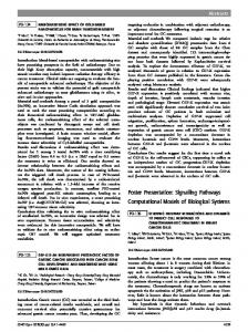
Fig. 1. A high-level model in the PEPA process algebra can be used to generate either a system of ODEs or a stochastic simulation

help to establish their relevance by reproducing the results of [1], starting from the published paper together with its supplementary material and the Matlab ODE model made available by the authors. We were able to reproduce the results from [1] starting from our model in the PEPA process algebra but because we were starting from the vantage point of modelling in process algebra we could apply other analysis procedures, unavailable to the authors of [1] (Figure 1). To our surprise when modelling in process algebra we discovered that the computational simulation conducted by ODEs in [1] contains a systematic flaw in the analysis process which affects many of the results, some significantly. To the best of our knowledge these errors are presently unknown: at the very least they were unknown to us. Using the insights obtained from our analysis procedures we were able to return to the differential equation model, diagnose and correct the flaws in the analysis, and show agreement between the results obtained using continuous-space analysis and the results obtained using a discrete-state stochastic analysis. Computational methods are well-understood to be complex and delicate so the relevance of this finding is not that there is an error in one particularly rich and valuable numerical study, or that modelling with ODEs is an unsatisfactory procedure, but rather that modelling in high-level languages (such as process algebras or Petri nets) may give a methodological advantage which allows an entire class of hard-to-detect errors and corner cases to be discovered and diagnosed before the results are published and promulgated to the wider scientific community. As original contributions the present paper contains the analysis of the process used to detect the error in the earlier modelling study [1], a description of the new software tool used for integrated continuous-space and discrete-state stochastic analysis of PEPA process algebra models, and an overview of an extensive process algebra modelling study comprising 188 process definitions describing the dynamics of 95 of the reaction channels in the signalling cascade of the EGF receptor-induced MAP kinase pathway. Structure of this paper: In Section 2 we present background material on our previous work. We follow this in Section 3 with a discussion of related work. In Section 4 we present an introduction to quantitative process algebras, considering

Stronger Computational Modelling of Signalling Pathways

65

the expressive capabilities of these languages. In Section 5 we explain how these languages are used in modelling. Section 6 presents a comparison of our analysis results and the results of other authors. In Section 7 we discuss the software tool used to perform the analysis. Finally, we present conclusions in Section 8.

2

Background

In an earlier study we made two distinct computational models of the Ras/Raf1/MEK/ERK signalling pathway, both expressed in the PEPA process algebra. Our models were based on the deterministic model presented directly as a system of coupled ordinary differential equations in [5]. Our process algebra models adhere to two distinct modelling styles—the reagent-centric and pathway models from [3]. We interpreted these under the continuous-time Markov chain semantics for the PEPA language, and thus these gave rise to stochastic models of the pathway. We used well-known procedures of numerical linear algebra to conduct a quantitative stochastic evaluation of the pathway. We used the process algebraic reasoning apparatus of the PEPA language to establish that these two models were strongly equivalent, meaning that a timing-aware observer could not distinguish between them. In the extension of this work in [6] we presented automatic procedures for converting in both directions between the reagent-centric and pathway views. We revisited the reagent-centric model in [4], mapping it to a system of ODEs. The model considered in [4] adds additional species to the model presented in [5] in order to concentrate on a detail of the pathway not considered in [5]. We applied the mapping procedure from [4] to a reduced version of the model without these additional species and were able to show that the model gave rise to exactly the same system of ODEs as studied previously in [5] establishing a precise formal equivalence between the process algebra model and the ODE model. The deterministic and stochastic approaches to computational modelling in systems biology are often presented as alternatives; one should choose one approach or the other. Some authors have suggested that stochastic approaches are technically superior because they can expose small-scale effects which are caused by some molecular species being present in the reaction volume in very low copy numbers. We are instead in agreement with the authors of [7], who argue that the principal challenge is choosing the appropriate framework for the modelling study at hand. For some problems the influence of effects such as intra-cellular noise or circumstances such as low copy numbers is sufficiently great that a thorough stochastic treatment is essential. In other modelling problems no such influences are manifest and a deterministic treatment based on reaction rate equations is the correct approach. The divergence between the stochastic behaviour exposed at low copy numbers of reactants and the deterministic approach based on reaction rate equations is due to the reliance of the ODE-based analysis on the assumption of continuity and the use of the law of mass action, essentially an empirical law derived from

66

M. Calder et al.

in vitro experimentation. Gillespie’s Stochastic Simulation Algorithm (SSA) [8] makes no use of such an empirical law, and is instead grounded in the theory of statistical thermodynamics. In consequence it is an exact procedure for numerically simulating the dynamic evolution of a chemically reacting system, even at low copy numbers. However, the SSA method converges, as the number of reactants increases, to the solution computed by the ODEs so that the methods are in agreement in the limit [9]. Gillespie’s exact algorithm models systems in which there are M possible reactions represented by the indexed family Rµ (1 ≤ μ ≤ M ). It builds on a reaction probability density function P (τ, μ | X) such that P (τ, μ | X)dτ is the probability that given the state X at time t, the next reaction in the volume will occur in the infinitesimal time interval (t + τ, t + τ + dτ ) and be an Rµ reaction. Starting from an initial state, SSA randomly picks the time and type of the next reaction to occur, updates the global state to record the fact that this reaction has happened, and then repeats. In practice, Gillespie’s SSA is effective only for non-stiff systems on short time scales. An approximate acceleration procedure called “τ -leaping” was later developed by Gillespie and Petzold [10]. The “implicit τ -leaping” method [11] was developed to attack the orthogonal problem of stiffness, common in multiscale modelling, where different time-scales are appropriate for reactions. Recent advances in the field include the development of slow-scale SSA which produces a dramatic speed-up relative to SSA by prioritising rare events [12]. A recent survey paper on stochastic simulation is [13]. A comparison paper on stochastic simulation methods and their relation to differential-equation based analysis of reaction kinetics is [9].

3

Related Work

We are not the first authors to investigate the model from [1] using stochastic simulation methods. An earlier comparison using the binomial τ -leap method appeared in [14]. However, the authors of [14] compare the solutions computed by their binomial τ -leap method with the solutions computed by Gillespie’s stochastic simulation algorithm and did not compare with the results from [1]. For this reason the authors of [14] did not find the error which we uncovered by comparing the results computed by stochastic simulation with the results computed by the authors of [1] using ordinary differential equations. In [15] the authors use the PRISM probabilistic model checker [16] to check logical formulae of Continuous Stochastic Logic (CSL) [17] against models of signalling pathways expressed as state-machines in the PRISM modelling language, comparing the result against an ODE model coded in the Matlab numerical platform. A recent technical note [18] uses modelling in a stochastic process calculus and stochastic simulation to investigate the MAPK cascade previously studied in [19] using ordinary differential equations. [18] uses synthetic values for rate constants (all are set to 1.0) so comparison with the results of [19] is not meaningful.

Stronger Computational Modelling of Signalling Pathways

4

67

Process Algebras

Process algebras are concise formally-defined modelling languages for the precise description of concurrent, communicating systems. Our belief is that they are well-suited to modelling cell signalling pathways and our interest here is exclusively in process algebras which are decorated with quantitative information [20]. The PEPA process algebra [2] which we use benefits from formal semantic descriptions of different characters which are appropriate for different uses. The structured operational semantics presented in [2] maps the PEPA language to a Continuous-Time Markov Chain (CTMC) representation. A continuous-space semantics maps PEPA models to a system of ordinary differential equations (ODEs) [21], admitting different solution procedures. 4.1

Expressiveness

Because we are modelling in a high-level language it is possible to apply these very different numerical evaluation procedures to compute different kinds of quantitative information from the same model. This is a freedom which we would not have if we had coded a Markov chain or a differential equation-based representation of the model directly in a numerical computing platform such as Matlab. One freedom which the use of a high-level language gives the modeller is the possibility to use either discrete-state or continuous-space analysis procedures. Another is the option of applying both types of analysis to the same model, and that is the approach which we have used here. One strength of the PEPA process algebra as an expressive and practical modelling language is its support for multi-way co-operation; we have made use of this expressive power in all of our modelling studies in systems biology. Genuinely tri-molecular collisions occur only exceptionally rarely in dilute fluids so these do not normally arise in our modelling for this reason. Rather a collision between, say, an enzyme and a substrate to produce a compound, is expressed in PEPA as a three-way co-operation between the input enzyme and substrate (whose molecular concentrations are reduced) and the output compound (whose molecular concentration is increased). Similarly a reaction channel with two input species and two output species is represented as a four-way co-operation in PEPA. Some reaction channels may have more inputs or more outputs and so having this expressive power available in our chosen process algebra seems well-suited to the type of modelling which is undertaken in the area. 4.2

Combinators of the Language

We give only a brief introduction to the PEPA language here. The reader is referred to [2] for the definitive description. PEPA provides a set of combinators which allow expressions to be built which define the behaviour of components via the activities that they engage in. These combinators are presented below.

68

M. Calder et al.

Prefix (α, r).P : Prefix is the basic mechanism by which the behaviours of components are constructed. This combinator implies that after the component has carried out activity (α, r), it behaves as component P . Choice P1 +P2 : This combinator represents a competition between components. The system may behave either as component P1 or as P2 . All current activities of the two components are enabled. The first activity to complete distinguishes one of these components and the other is then discarded.


P2 : This describes the synchronization of components P1 Cooperation: P1  L and P2 over the activities in the cooperation set L. The components may proceed independently with activities whose types do not belong to this set. A particular case of the cooperation is when L = ∅. In this case, components proceed with all activities independently. The notation P1  P2 is used as a shorthand for
P1  P2 . In a cooperation, the rate of a shared activity is defined as the rate of ∅ the slowest component. Hiding: P/L This component behaves like P except that any activities of types within the set L are hidden, i.e. such an activity exhibits the unknown type τ and the activity can be regarded as an internal delay by the component. Such an activity cannot be carried out in cooperation with any other component: the original action type of a hidden activity is no longer externally accessible, to an observer or to another component; the duration is unaffected. Constant: A = P Constants are components whose meaning is given by a def defining equation: A = P gives the constant A the behaviour of the component P . This is how we assign names to components (behaviours). An explicit recursion operator is not provided but components of infinite behaviour may be readily described using sets of mutually recursive defining equations. def

5

Modelling

For this system we developed a reagent-centric model. In this style of modelling we associate a distinct PEPA component with each reagent in the system. This is a more abstract mapping than is used in most of the work using stochastic π-calculus [22], where a distinct component is associated with each molecule in the system. In the reagent-centric style, we represent the state of the system as the conjunction of the states of the components, each local state corresponding to a concentration level of an individual reagent. Concentration levels are discretized and the local states of the PEPA component records the impact of each possible reaction on the concentration level. The impact will depend on the role that the reagent plays within this particular reaction. This is summarised in Table 1. Enzymatic reactions are possible when the enzyme is present in high concentration, and have no impact on the amount of enzyme although the current concentration of the enzyme will affect the rate of reaction. Conversely for inhibitory reactions: the inhibitor must be in low concentration and will remain low and its concentration has a regulatory effect on the rate of the reaction.

Stronger Computational Modelling of Signalling Pathways

69

Table 1. The impact and role of reagents

Reagent role Impact on reagent Impact on reaction rate Producer decreases concentration has a positive impact, i.e. proportional to the current concentration level Product increases concentration has no impact on the rate, except at saturation Enzyme concentration unchanged has a positive impact, i.e. proportional to current concentration Inhibitor concentration unchanged has a negative impact, i.e. inversely proportional to current concentration

A PEPA model in this style can be thought to define a schematic for the possible reactions in the system. In the ODE mapping the local states represent the concentrations of the reagents. In the mapping to stochastic simulation, the local states indicate the types of molecules involved in the reactions and this is automatically mapped to a chemical master equation representation suitable for simulation using Gillespie’s algorithm. Figure 2 shows a small network, and the PEPA reagent-centric model that describes the graphical representation. In this example the PEPA components are A, B and C, and are tagged with H and L to designate the high and low concentrations, the coarsest possible discretization. The PEPA equations record the impact of each reaction on the concentration of that reagent.

b_a A

ab_c

c_a

B

c_b

AH AL BH BL CH CL

= (ab c, α).AL def = (b a, β).AH +(c a, γ).AH def = (ab c, α).BL +(b a, β).BL def = (c b, δ).BH def = (c a, γ).CL +(c b, δ).CL def = (ab c, α).CH

C

(AH

def




{ab c,b a}

BH ) {ab




c,c a,c b}

CL

Fig. 2. PEPA reagent-centric example

ab c, A + B → C , α b a, B → A ,β

c b, C → B , δ c a, C → A , γ

Fig. 3. An equivalent model in chemical reaction language

The PEPA definitions in Figure 2 give rise to four reactions shown in Figure 3 in the chemical reaction language format W, X → Y, Z. W is the name for the reaction, X = {X1 + ... + Xn } lists all the components that are consumed in

70

M. Calder et al.

this named reaction. Y is a list in the same format as X representing those components that are increased by this reaction. The last part of the reaction, Z, defines a rate constant from which the reaction rate is derived. The reaction ab c consists of two reactants and one product. From the PEPA definition in Fig. 2, components A and B transition from a high to low state via the activity/reaction ab c: they are the two reactants of reaction ab c. Similarly, component C transitions from a low to high state by reaction ab c: it is the product of this reaction. This form of reasoning is used to transform all the PEPA equations into chemical reaction language format. The rate of each reaction is not simply the defined constant. Where previously the reaction ab c was defined as A + B → C, α, we take the constant α and multiply it by the number of molecules in both the A and B components (to allow for all permutations) to give a reaction rate of αAB, the mass action rate. As outlined above, both stochastic simulation and ODE analysis are available. ODEs derived from PEPA in this manner will always respect the rules of conservation, as PEPA works on a static number of components. The inclusion of stoichiometric information outside of the PEPA model does however allow for a more powerful representation. In this case the numbers of each components required in each reaction are any valid integer i.e. ab c requires 3 units of component A instead of 1. 5.1

Schoeberl Model in PEPA

In attempting to reproduce the model created by Schoeberl et al., the main source of information came from the supplementary material to [1]. The complexity of the model highlights the issues surrounding graphical representations as can be seen in Fig. 4. The reaction v7, highlighted in blue is a uni-directional reaction and shows one instance of internalisation. Other reactions such as v2, v3 are bi-directional yet with no obvious difference within the graphical scheme. Additional information in the form of tabled reactions and rates, for example v7,

[(EGF-EGFR∗ )2] → [(EGF-EGFRi∗ )2]

can resolve some of the ambiguities, and by making joint use of these two representations the PEPA model can be constructed. Each component is taken in turn, with each reaction it participates in recorded against it. If we use (EGF-EGFR)2 (which can be seen in Fig. 4) as an example; (EGF-EGFR)2 can become phosphorylated (v3) and form (EGF-EGFR∗ )2, and this autophosphorylation can be reversed. This information would allow us to construct a definition such as that presented in equation (1). EGF-EGFR2H = (v3, k3).EGF-EGFR2L def

EGF-EGFR2L = (v-3, k-3).EGF-EGFR2H def

(1)

Stronger Computational Modelling of Signalling Pathways

71

Fig. 4. An extract of the signalling pathway (reproduced from [1])

Going further, we realise that (EGF-EGFR)2 is formed from the dimerization of EGF-EGFR (v2) and that this step can also be reversed. Adding this information to the previous definitions produces the definitions shown in (2). EGF-EGFR2H = (v3, k3).EGF-EGFR2L + (v-2, k-2).EGF-EGFR2L def

EGF-EGFR2L = (v-3, k-3).EGF-EGFR2H + (v2, k2).EGF-EGFR2H def

(2)

In this manner, each component can be built up to form the complete model. Some of the more complex compounds, such as (EGF-EGFR∗ )2-GAP-Shc∗ Grb2-Sos, participate in nine reactions creating large definitions. The definitions are structurally similar, consisting of multiple choice operators for the prefixes. This brief description can account for the majority of the model but not all. The dimerization process seen in reactions v9 and v11 currently require the addition of stoichiometric information. Through the interface to our software tool (described in Section 7) you can stipulate that two EGF-EGFR complexes form one (EGF-EGFR)2. When converting to Matlab this is translated to dy(3) = −2k2 y(3)2 dy and dy(4) = k2 y(3)2 dy where y(3) is EGF-EGFR and y(4) is (EGF-EGFR)2. Certain complexes can degrade such as EGFRi and EGFi, forming components that only increase in volume. The final behaviour that requires consideration is that of EGF. EGF binds to the EGF receptors, circled in red on the left in Fig. 4. The reactions present within [1] all suggest that EGF is consumed in this binding. This is not the case and in the Matlab model the rate of change for EGF is set to zero for all reactions it is involved in. This can be likened to a reservoir: the EGF is present at a given concentration but there exists so much at this level that the reduction is negligible. In the PEPA model this must be made explicit from the start. The

72

M. Calder et al.

influence of EGF can be defined either as a secondary rate parameter, effectively increasing the rate at which the reaction will take place, or EGF can be defined as a catalyst in the relevant reactions. In the PEPA model the catalytic route def was taken and so defined as EGFH = (v1, k1).EGFH .

6

Comparison

Figure 5 shows the time series plots for the six components highlighted in the original Schoeberl et al. paper. Each graph has three time series plots: 1. the solution of the original model1 from [1] which is a Matlab program which specifies a fixed time step and solution using the ode15s procedure from the Matlab ODE suite [23]; 2. the result of a τ -leap simulation of our PEPA model; and 3. the solution of an amended version of the original model using smaller time steps with the ode15s procedure. Each form of analysis was run for the same duration (60 minutes) in order to replicate the results of the original model as closely as possible. Of the six components MEK-PP, Raf∗ and Ras-GTP spike in a short space of time, and so to more readily show the differences the time series were cut short once the rate of change had dropped off towards zero. The use of the particular step within the solver is most apparent in Ras-GTP. The original model’s results indicate a peak at two minutes with a value of 8000 molecules/cell. The true peak occurs earlier, reaching double the original value at 16,000 molecules/cell. As can be seen, the value at two minutes is correct, but that the speed at which this component changes means the bulk of the reaction has already taken place, and the analysis incorrectly steps over the true peak onto the negative gradient of the curve. Differences can be seen also within the Raf∗ and to a lesser extent MEK-PP. In all of the graphs, it is nearly impossible to distinguish the τ -leap and variable-step ode15s solver at this resolution. This discrepancy only became apparent when comparing the results from the stochastic simulation and that of the ODE analysis, and we were only in a position to compare these alternative models because we generated both from a high-level process algebra description. Prior to running the τ -leap simulation, the arguments for the ODE analysis of the PEPA model had been extracted from the original model. Hence the same results were obtained, with the peaks in identical places. The time taken to solve the ODE model using the stiff solver with smaller time steps was almost identical to the time taken to solve model with fixed larger time steps. The time taken to solve the model using the τ -leap method is longer than the time taken to solve the model using Matlab’s stiff ODE solver (ode15s) but shorter than the time required by a standard solver such as ode45. 1

Available on-line at http://web.mit.edu/dllaz/egf pap/

Stronger Computational Modelling of Signalling Pathways (EGF-EGFR*)2 50000

1e+07 Molecules per Cell

40000 Molecules per Cell

ERK-PP 1.2e+07

Original Schoeberl et al. Matlab model PEPA derived Tau-leap simulation Schoeberl et al. model - smaller steps

45000 35000 30000 25000 20000 15000 10000

8e+06 6e+06 4e+06 2e+06

Original Schoeberl et al. Matlab model PEPA derived Tau-leap simulation Schoeberl et al. model - smaller steps

5000 0

0 0

10

20

30

40

50

60

0

10

20

30

Time (min)

Molecules per Cell

Molecules per Cell

14000

120000 100000 80000 60000

12000 10000 8000 6000

40000

4000

20000

2000

0

0 0

5

10

15

20

0

2

4

Time (min)

90000 80000 Molecules per Cell

12000 10000 8000 6000

70000 60000 50000 40000 30000

4000

20000

2000

10000

0

Original Schoeberl et al. Matlab model PEPA derived Tau-leap simulation Schoeberl et al. model - smaller steps

0 4

10

SHC

14000

2

8

100000

Original Schoeberl et al. Matlab model PEPA derived Tau-leap simulation Schoeberl et al. model - smaller steps

16000

6

Time (min)

Ras-GTP 18000

Molecules per Cell

60

Original Schoeberl et al. Matlab model PEPA derived Tau-leap simulation Schoeberl et al. model - smaller steps

16000

140000

0

50

Raf* 18000

Original Schoeberl et al. Matlab model PEPA derived Tau-leap simulation Schoeberl et al. model - smaller steps

160000

40

Time (min)

MEK-PP 180000

73

6

Time (min)

8

10

0

10

20

30

40

50

60

Time (min)

Fig. 5. Graphs of differential equation and stochastic simulation results compared. The solid red line is the solution of the original model from [1], which shows marked differences in some graphs from the solution of the PEPA-derived τ -leap simulation and (a dashed green line) and the solution of the ODE model using smaller time steps (a dotted blue line). The solution of the PEPA-derived τ -leap simulation and the solution of the ODE model using smaller time steps are virtually indistinguishable in the graphs.

7

Implementation

The reason to have a formally-defined high-level language for performance modelling is that it is possible to implement software tools which evaluate models according to the formal semantics of the language. For the present study we

74

M. Calder et al.

produced a tool platform to support the compilation of PEPA models in the reagent-centric style by extending the Choreographer platform [24] which we developed for general quantitative analysis of PEPA models. Choreographer is an integrated development environment for process algebraic modelling, comprising a language-sensitive editor for PEPA and a toolbox of solution procedures for continuous-time Markov chains. We extended Choreographer to communicate with the publicly-available ISBJava library for stochastic simulation as used by the Dizzy [25] chemical kinetics stochastic simulation software package. We also extended Choreographer to communicate with the Matlab numerical computing platform, which we use for numerical integration of ODEs. A screenshot of our extended Choreographer platform appears in Figure 6.

Fig. 6. The Choreographer quantitative development and analysis platform

8

Conclusions

Errors in the use of typical computing applications frequently manifest themselves as a null pointer dereference or a segmentation fault: the application tells the user that an error has occurred. Errors in the use of numerical computing routines are more insidious than errors in typical computing. No memory faults are signalled and the application often completes normally within the anticipated duration of run, delivering a plausible graph of analysis results. Without any such alarm bells being sounded the modeller must always be on guard to look for potential traps such as an over-generous step-size and it is entirely forgivable if they cannot always do this for every graph in every modelling study.

Stronger Computational Modelling of Signalling Pathways

75

Rather than place this intellectual burden on the modeller we would prefer to use stronger computational modelling procedures which would routinely apply both continuous-state analysis methods (such as ODE solution) and discretestate analysis (such as stochastic simulation). High-level modelling languages such as the PEPA process algebra are helpful here. Instead of coding the differential equations and the stochastic simulation directly we generate these from a single process algebra model, gaining the value of the application of both types of analysis without the expense of any re-implementation. Using this approach we uncovered a flaw in the results presented in [1]. We had no a priori reason to suspect that there was a flaw; comparing the stochastic simulation results to the ODE solution identified a clear problem, at a modest computational cost. All computations were done on a single desktop PC. We believe that the insights obtained from this study stand as a good advertisement for the usefulness of high-level modelling languages for analysing complex biological processes whether process algebras, Petri nets or SBML [26]. We compared in Figure 5 the analysis results obtained by solution of the differential equations with the solutions computed by stochastic simulation. As is typical for stiff systems, some effects are best considered over different time scales. Some species (such as ERK-PP and SHC) exhibit high concentration for a period of hours. Others (such as Raf∗ and Ras-GTP) peak within minutes. The large time step used in the computation in [1] is not a problem for the analysis of the long-lived species but gives misleading results for those species which are short-lived. We discovered very good agreement between the results calculated by the τ leap method and the results calculated from the differential equations when a variable timestep is used. The solution of the variable timestep ODEs agrees almost exactly everywhere with the solution obtained from Gillespie’s approximate τ -leap method: these two lines are overlapping on the plots in Figure 5. Acknowledgements. Muffy Calder and Adam Duguid are supported by the DTI Beacon Bioscience Projects programme. Stephen Gilmore and Jane Hillston are supported by the EU IST-3-016004-IP-09 project SENSORIA. Jane Hillston is supported by the Engineering and Physical Sciences Research Council Advanced Research Fellowship EP/C543696/1 “Process Algebra Approaches to Collective Dynamics”. The authors acknowledge helpful discussions with Richard Orton of the Bioinformatics Research Centre, University of Glasgow on aspects of the computational modelling of the MAPK pathway.

References 1. B. Schoeberl, C. Eichler-Jonsson, E.D. Gilles, and G. Muller. Computational modeling of the dynamics of the MAP kinase cascade activated by surface and internalized EGF receptors. Nature Biotechnology, 20:370–375, 2002. 2. J. Hillston. A Compositional Approach to Performance Modelling. Cambridge University Press, 1996.

76

M. Calder et al.

3. Muffy Calder, Stephen Gilmore, and Jane Hillston. Modelling the influence of RKIP on the ERK signalling pathway using the stochastic process algebra PEPA. In Anna Ingolfsdottir and Hanne Riis Nielson, editors, Proceedings of the BioConcur Workshop on Concurrent Models in Molecular Biology, London, England, August 2004. 4. Muffy Calder, Stephen Gilmore, and Jane Hillston. Automatically deriving ODEs from process algebra models of signalling pathways. In Gordon Plotkin, editor, Proceedings of Computational Methods in Systems Biology (CMSB 2005), pages 204–215, Edinburgh, Scotland, April 2005. 5. K.-H. Cho, S.-Y. Shin, H.-W. Kim, O. Wolkenhauer, B. McFerran, and W. Kolch. Mathematical modeling of the influence of RKIP on the ERK signaling pathway. In C. Priami, editor, Computational Methods in Systems Biology (CSMB’03), volume 2602 of LNCS, pages 127–141. Springer-Verlag, 2003. 6. Muffy Calder, Stephen Gilmore, and Jane Hillston. Modelling the influence of RKIP on the ERK signalling pathway using the stochastic process algebra PEPA. Transactions on Computational Systems Biology, 2006. Extended version of [3]. To appear. 7. O. Wolkenhauer, M. Ullah, W. Kolch, and K.-H. Cho. Modelling and simulation of intracellular dynamics: Choosing an appropriate framework. IEEE Transactions on Nanobioscience, 3(3):200–207, September 2004. 8. D.T. Gillespie. Exact stochastic simulation of coupled chemical reactions. Journal of Physical Chemistry, 81(25):2340–2361, 1977. 9. T.E. Turner, S. Schnell, and K. Burrage. Stochastic approaches for modelling in vivo reactions. Computational Biology and Chemistry, 28:165–178, 2004. 10. D.T. Gillespie and L.R. Petzold. Improved leap-size selection for accelerated stochastic simulation. J. Comp. Phys., 119:8229–8234, 2003. 11. M. Rathinam, L.R. Petzold, Y. Cao, and D.T. Gillespie. Stiffness in stochastic chemically reacting systems: The implicit tau-leaping method. Journal of Chemical Physics, 119(24):12784–12794, December 2003. 12. Y. Cao, D.T. Gillespie, and L. Petzold. Accelerated stochastic simulation of the stiff enzyme-substrate reaction. Journal of Chemical Physics, 123:144917–1 – 144917– 12, 2005. 13. D. Gillespie and L. Petzold. System Modelling in Cellular Biology, chapter Numerical Simulation for Biochemical Kinetics. MIT Press, 2006. Ed. Z. Szallasi, J. Stelling and V. Periwal. 14. Abhijit Chatterjee, Kapil Mayawala, Jeremy S. Edwards, and Dionisios G. Vlachos. Time accelerated Monte Carlo simulations of biological networks using the binomial τ -leap method. Bioinformatics, 21(9):2136–2137, 2005. 15. M. Calder, V. Vyshemirsky, D. Gilbert, and R. Orton. Analysis of signalling pathways using the PRISM model checker. In Gordon Plotkin, editor, Proceedings of Computational Methods in Systems Biology (CMSB 2005), Edinburgh, Scotland, April 2005. 16. M. Kwiatkowska, G. Norman, and D. Parker. PRISM: Probabilistic symbolic model checker. In A.J. Field and P.G. Harrison, editors, Proceedings of the 12th International Conference on Modelling Tools and Techniques for Computer and Communication System Performance Evaluation, number 2324 in Lecture Notes in Computer Science, pages 200–204, London, UK, April 2002. Springer-Verlag. 17. A. Aziz, K. Sanwal, V. Singhal, and R. Brayton. Model checking continuous time Markov chains. ACM Transactions on Computational Logic, 1:162–170, 2000.

Stronger Computational Modelling of Signalling Pathways

77

18. Luca Cardelli. Mapk cascade. Microsoft Research Cambridge UK technical note. Available on-line at http://research.microsoft.com/Users/luca/Notes/Mapk Cascade.pdf, July 2005. 19. Chi-Ying F. Huang and James E. Ferrell Jr. Ultrasensitivity in the mitogenactivated protein kinase cascade. Biochemistry, 93(19):10078–10083, September 1996. 20. J. Hillston. Process algebras for quantitative analysis. In Proceedings of the 20th Annual IEEE Symposium on Logic in Computer Science (LICS’ 05), pages 239– 248, Chicago, June 2005. IEEE Computer Society Press. 21. J. Hillston. Fluid flow approximation of PEPA models. In Proceedings of the Second International Conference on the Quantitative Evaluation of Systems, pages 33–43, Torino, Italy, September 2005. IEEE Computer Society Press. 22. C. Priami, A. Regev, W. Silverman, and E. Shapiro. Application of a stochastic name passing calculus to representation and simulation of molecular processes. Information Processing Letters, 80:25–31, 2001. 23. Lawrence F. Shampine and Mark W. Reichelt. The Matlab ODE suite. SIAM J. Sci. Comput., 18(1):1–22, 1997. 24. Mikael Buchholtz, Stephen Gilmore, Valentin Haenel, and Carlo Montangero. Endto-end integrated security and performance analysis on the DEGAS Choreographer platform. In I.J. Hayes J.S. Fitzgerald and A. Tarlecki, editors, Proceedings of the International Symposium of Formal Methods Europe (FM 2005), number 3582 in LNCS, pages 286–301. Springer-Verlag, June 2005. 25. S. Ramsey, D. Orrell, and H. Bolouri. Dizzy: stochastic simulation of large-scale genetic regulatory networks. J. Bioinf. Comp. Biol., 3(2):415–436, 2005. 26. M. Hucka, A. Finney, H. M. Sauro, H. Bolouri, J. C. Doyle, and H. Kitano et al. The systems biology markup language (SBML): a medium for representation and exchange of biochemical network models. Bioinformatics, 19(4), 2003.