sentence-level log linear models is proposed for ASR. This form of model is shown to be similar to the recently proposed structured. SVM. Second, based on the ...
1
Structured Log Linear Models for Noise Robust Speech Recognition Shi-Xiong Zhang, Anton Ragni, Student Member, IEEE, and Mark Gales, Senior Member, IEEE
Abstract—The use of discriminative models for structured classification tasks, such as speech recognition is becoming increasingly popular. This paper examines the use of structured loglinear models for noise robust speech recognition. An important aspect of log-linear models is the form of the features. By using generative models to derive the features, state-of-the-art model-based compensation schemes can be used to make the system robust to noise. Previous work in this area is extended in two important directions. First, a large margin training of sentence-level log linear models is proposed for ASR. This form of model is shown to be similar to the recently proposed structured SVM. Second, based on the designed joint features, efficient lattice-based training and decoding are performed. This novel model combines generative kernels, discriminative models, efficient lattice-based large margin training and model-based noise compensation. It is evaluated on a noise corrupted continuous digit task: AURORA 2.0.
Index Terms: Speech recognition, large margin training, discriminative models, structured SVM. I. I NTRODUCTION Automatic speech recognition (ASR) is usually based on generative models, in the form of Hidden Markov Models (HMMs) and class priors, the language models. Although improvements have been observed from using discriminative criteria for training HMMs [1], [2], the underlying models of these systems are still generative, with the class posteriors being produced using Bayes’ rule. This has led to interest in discriminative models and discriminant functions for ASR. In discriminative models, e.g., Conditional Random Fields (CRF) [3], logistic regression machines [4], and Conditional Augmented models (C-Aug) [5], the posterior of the wordsequence given the observation are directly modelled. For these discriminative models a number of important decisions need to be made, including: the form of the features to use; how to handle continuous speech; and the appropriate training criterion. This paper describes possible solutions to these problems that enable discriminative models to be used for noise robust recognition of continuous digits. Approaches have previously been published to all these problems. A number of features have been proposed, both at the frame level, and based on generative models [6]. Approaches for incorporating structure have been based on lattice approaches [3], [5] or by segmenting the data [7]. Discriminative models are often trained using Conditional Maximum Likelihood [3]–[5]. However for high-dimensional S.-X. Zhang, A. Ragni, and M.J.F. Gales are with the Cambridge University Engineering Department, Trumpington St., Cambridge CB2 1PZ, U.K. (email: {sxz20, ar527, mjfg}@eng.cam.ac.uk). The authors thank Toshiba Cambridge Reseach Lab. and the HTK projects for part-funding this work.
features, especially with limited training data, there may be issues with generalisation. Also the training criterion is not linked with the evaluation criterion. To address this there has been interest in large margin [8] and minimum Bayes’ risk [1] criteria. To address the issue of noise robustness with discriminative models, the concept of adapting the kernels associated with SVMs has been used [7]. This paper proposes a structured log-linear model with large margin training for noise robust continuous ASR. The features are derived from generative kernels, which provides an elegant way of combining generative and discriminative models to handle time-varying data. Additionally, since the features are based on the generative models, model-based compensation can be easily performed for noise robustness [9]. Instead of using CML training, this paper describes efficient large margin training based on lattices. This form of model is shown to be related to both multi-class SVMs and structured SVMs. The performance of the system is compared to a number of existing approaches on the AURORA 2 task. II. S TRUCTURED L OG L INEAR M ODELS Given an observation sequence, O = {o1 , . . . , oT }, the posterior of the hypothesised labels w for many discriminative models can be expressed as a member of exponential family, ¡ ¢ 1 exp αT φ(O, w; λ) , (1) P (w|O; α, λ) = Z(O; α, λ) where w may P represent¡ a sequence or¢ an isolated label, T Z(O; α, λ) = w exp α φ(O, w; λ) is the normalisation term and α are the discriminative model parameters. φ(O, w; λ) is a joint feature space which models the dependencies and underlying structures between O and w. λ are the parameters used for constructing joint features. Recognition with this form of model can simply be expressed as ˆ = arg max P (w|O; α, λ) = arg max αT φ(O, w; λ). (2) w w
w
Deriving an appropriate joint feature space is one of the key aspects of applying log-linear models (Eq. 1) to a specific task. For ASR, since the observations O have variable length, the joint feature space should map the dynamic length sequences to a fixed dimensional vector. For some tasks it is possible to directly use the joint feature space, unstructured data case. However for tasks such as continuous speech recognition, where the number of possible sentence labels is very large, structure must be introduced into the features. In common with standard speech recognition a common set of basic structure units, e.g. words or phones, are specified. These are then combined together in different sequences to yield all possible sentences.
2
A. Joint Feature Space for Unstructured Data For situations where there are a small number of possible labels, or the data can be segmented so that the number of labels is small, unstructured joint feature spaces can be used. For each segment, feature spaces related to sequence kernels can be used to handle the dynamic mapping. Of particular interest in this work are those kernels based on generative models. As well as yielding a well motivated dynamic mapping, these generative kernels allow standard speaker and noise adaptation approaches developed for ASR to be used to derive robust features. Given an observation-label pair (O, w), there are a number of possible feature-spaces that can be used to form the joint feature space. One form used for C-Aug models [5] is .. . ¡ ¢ (w ˜k ) ∇ log p(O; ) ϕ (O; λ) = (3) ¡ λ ¢ , ( w ˜ ) k ∇λ(w˜k ) log p(O; λ ) .. . where {w ˜k }M k=1 denotes all possible words (or phones) in the dictionary, p(O; λ(w˜k ) ) is a likelihood of observations O for model w ˜k , and ∇λ denotes the first-order derivatives with respect to λ. There are a number of elegant properties of this form of model, including modifying the form of the conditional independence assumptions. A simpler example of generative kernel-induced feature spaces is the log-likelihood feature space [4], [6] ¡ ¢ log p(O; λ(w˜1 ) ) .. ϕLL (O; λ) = (4) . ¡ ¢ . (w ˜M ) log p(O; λ ) To model the dependencies between observations O and unstructured label w, based on the feature space ϕLL (O; λ) the joint feature space is defined as φ(O, w; λ)|w=w = T1 δ(w) ⊗ ϕLL (O; λ) =
1 T
T
LL
T
(5)
δ(w) = [δ(w − w ˜1 ), . . . , δ(w − w ˜M )]T T
T
α = [α(w˜1 ) , . . . , α(w˜k ) , . . . , α(w˜M ) ]T where ⊗ is the tensor product, the index of ϕLL (O; λ) in the sparse feature vector φ(O, w; λ) depends on the position of (w ˜ ) (w ˜ ) (w ˜k ) w in the dictionary {w ˜k }M = [α1 k , . . . , αM k ] k=1 , and α are the parameters with class w ˜k . One can easily further write αT φ(O, w; λ)|w=w =
1 T
T
L ¡ ¢ 1P δ(wi ) ⊗ ϕLL (Ot(wi ,θ) ; λ) (7) T i=1 £ ¤ T PL ˜1 ) ϕLL (Ot(wi ,θ) ; λ) i=1 δ(wi − w 1 .. . T £ LL ¤ PL ˜M ) ϕ (Ot(wi ,θ) ; λ) i=1 δ(wi − w
αT φ(O, w; θ, λ) = αT =
α(w˜1 ) .. . α(w˜M )
where ϕLL (Ot(wi ,θ) ; λ) is defined in Eq. 4. Unlike the unstructured case in Section II-A, this joint feature space is not sparse. One interesting property of this joint feature space is that if all (w ˜ ) the α(w˜k ) = [0, . . . , αk k , . . . , 0] in α, then αT φ(O, w; θ, λ) can be expressed as the summation of scaled log likelihoods of each word. Unlike acoustic or language model weighting, where a constant scalar is used [1], the scalars here become (w ˜ ) class-dependent, αk k , and can be trained under any of the criteria discussed in Section III. For a specific pair (O, w), theoretically all possible alignments should be considered. However, for efficient training and decoding, only the “most likely” alignment θˆ is considered. This is selected using Viterbi searching based on the generative models, θˆ = arg max P (θ)p(O1:T |θ, λ(w) ). θ
(8)
ˆ the utterance-based joint Given this “most likely” alignment θ, feature space in Eq. 1 can be approximated by setting ˆ λ). αT φ(O, w; λ) ≈ αT φ(O, w; θ,
(9)
T T
[0 , . . . , ϕ (O; λ) , . . . , 0 ] T
this problem, the labels are decomposed into shared structure units (words). Thus, an additional level of latent variables that represent the alignment is introduced. Consider a dictionary of M words, and let θ denote the alignment that splits the observation sequence O1:T into L segments O1:T = {Ot(w1 ,θ) , . . . , Ot(wi ,θ) , . . . , Ot(wL ,θ) }. Given one such alignment the joint feature space for the observation-label pair (O, w) can be defined as
α(w) ϕLL (O; λ).
(6)
III. D ISCRIMINATIVE T RAINING In addition to designing an appropriate joint feature space, another important decision for structured log-linear models is the training criterion. Discriminative models can be trained under the conditional maximum likelihood (CML) or Minimum Bayes’ Risk (MBR) criteria. In the CML training, the following form is maximised [1] R 1 X (r) Fcml (α, λ) = log(P (wref |O(r) ; λ, α)), (10) R r=1
Thus the joint feature space defined in Eq. 5 can be integrated into the log-linear model (Eq. 1). This yields a consistent feature-space for all classes, ϕLL (O; λ), with class specific parameters α(w) . To avoid the long utterances dominating the training, joint feature spaces in this work are normalized by the number of frames T .
where O(r) is the rth training utterance with transcription (r) wref . CRF [3] and C-Aug [5] were trained under this criterion. An alternative to CML is MBR where the expected loss is minimised R 1 XX (r) P (w|O(r) ; λ, α)L(w, wref ) (11) Fmbr (α, λ) = R r=1 w
B. Joint Feature Space for Structured Data
and L(w, wref ) is a suitable loss function, e.g., 0/1 loss or Levenshtein distance between the reference and hypothesis. In ASR, since the underlying models are usually not known and the training data is always limited, CML and MBR-type
For general continuous speech recognition, given observations O, the number of possible classes, i.e., hypothesized sentences w could be exponential large. To handle
(r)
3
training criteria may have overtraining issues. In order to train a robust classifier capable of generalizing well even on high-dimension space with limited data, large margin based approaches have become popular [2], [8]. This criterion can be extended to the of interest model by minimising 1 Flm (α, λ) = · (12) R !)# " ( Ã R (r) X P (wref |O(r) ; λ, α) (r) max L(w, wref ) − log (r) P (w|O(r) ; λ, α) r=1 w6=wref +
where [ ]+ is the hinge-loss function. In Eq. 12 the margin is defined by the log posterior ratio between wref and the best competing hypothesis w. One general extension of this criterion is to incorporate priors P (α), P (λ): F(α, λ) = Flm (α, λ) − log (P (α)) − log (P (λ)) .
(13)
In this work the base model parameters, λ, are assumed to have been trained. Eq. 12 can then be expressed as R 1 Xh (r) − log P (wref |O(r) ; λ, α) FLM (α) = − log (P (α)) + R r=1 # n ³ ´o (r) (r) + max L(w, wref ) + log P (w|O ; λ, α) (14) (r)
w6=wref
+
(m)T Σ(m) = J(m) Σ(m) + (I − J(m) )Σn (I − J(m) )T(17) x J (m)
(m)
where µx and Σx are the “clean” speech component mean vector and covariance matrix, and µn , Σn and µh are the additive and convolutional noise parameters respectively. C is the DCT matrix and J(m) is Jacobian matrix [9]. exp() and log() are element-wise exponential and logarithm respectively. The noise model parameters are estimated using maximum likelihood estimation [12]. Thus in this work discriminative model parameters are assumed to be noise-independent, whereas the generative model parameters are noise-dependent. V. E XPERIMENTS
For this work, Gaussian prior P (α) = N (α; µα , Σα ) with a zero mean and scaled identity covariance matrix, µα = 0 and Σα = CI will be used. Substituting Eq. 1 into Eq. 14, yields the following regularized form R 1 C Xh (r) FLM (α) = ||α||22 + −αT φ(O(r) , wref ; λ) + (15) 2 R r=1 n o¸ (r) T (r) max L(w, wref ) + α φ(O , w; λ) w6=wref
options. First, the discriminative model parameters, αT = T T [α(w˜1 ) , . . . , α(w˜M ) ], can be modified to be noise dependent. However with very limited data in the target domain, in these experiments a single utterance, this is not possible. Alternatively, the parameters λ associated with the generative feature space are modified [7]. This can be achieved using any model-based compensation scheme. In this work VTS is used. Considering just the static components of the acoustic models, the compensated mean vector and covariance matrix of component m of the generative model are given by ³ ´ -1 µ(m) = C log exp(C-1 (µ(m) + µ ) + exp(C µ ) (16) h n x
+
Note in this form the normalization term Z(O; α, λ) has been canceled out, so no longer appears in training or recognition. The structural log-linear model in this work is trained using this large margin criterion (Eq. 15). This criterion results in different forms of model depending on whether the structured or unstructured cases from Section II are being considered. For the structured case where the general form of Eq. 15 is used, the criterion is the same as the training criterion for Structure SVMs (SSVMs) [10]. For the unstructured case, the training data from the same utterance but belonging to a different segmentation are treated independently. As a result, a log linear model with the joint feature space in Eq. 6 trained using the large margin criterion (Eq. 15) is the same as a Multi-class SVM (MSVM) [11], where α(w) and ϕLL (O; λ) in Eq. 6 are the class-dependent MSVM parameters and class-independent feature space. IV. N OISE ROBUSTNESS In ASR, the acoustic conditions during training and testing are seldom matched. For standard generative models, modelbased compensation schemes such as Vector Taylor Series (VTS) compensation [9] are a popular and successful approach to handling this problem. When applying the same concept to the log-linear models in this work there are two
The performance of the proposed model was evaluated on the AURORA 2 task. AURORA 2 is a standard small vocabulary digit string recognition task. The vocabulary size M is only 12 (one to nine, plus zero, oh and silence). The utterances in this task are one to seven digits long based on the TIDIGITS database with noise artificially added. The 8440 clean mix-gender training utterances were used to train the acoustic generative models (HMMs). 39 dimensional observations consisting of 12 MFCCs appended with the zeroth cepstrum, delta and delta-delta coefficients were used in this work. The “simple” back-end was used, thus the HMMs were 16 emitting states whole word digit models, with 3 mixtures per state and silence and inter-word pause models. Test set A was used as the development set for tuning parameters for all systems, such as the penalty factor C for SVMs. All three test sets, A, B and C, were used for evaluation. The parameters of the log linear models were trained using the same subset of the multi-condition training data as [7]: three of the four subsets (N2-N4) and three of five SNRs (10dB, 15dB, 20dB). This allows direct comparison with the previously published results. In this work lattices, generated from the noise compensated acoustic models, were used during both training and recognition. For training it is necessary to obtain the “best competing” hypothesis (the max {·}) for Eq. 15. Similar w6=wref
to the discriminative training in [1], the loss of a hypothesis (corresponding to a path in the lattice) is approximated by accumulating the alignment-based local loss on each arc along the path in the lattice. As the joint feature space (Eq. 7) can also be decomposed at the word level, this allows the “best competing” hypothesis in Eq. 15 to be efficiently found via an arc-level forward-backward combined with Viterbi search over the lattice (For more details see [13]). For recognition the
4
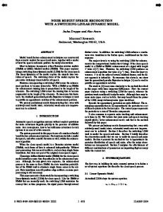
SNR (dB) 20 15 10 05 00 Avg
HMM 1.69 2.36 4.39 11.20 29.55 9.84
Test Set A SVM MSVM 1.51 1.50 2.11 1.98 3.86 3.63 10.02 9.16 28.00 25.09 9.10 8.27
SLLM 1.25 1.76 3.33 8.66 23.90 7.78
TABLE I P ERFORMANCE (WER %) OF VTS BASED HMM, SVM, MSVM AND STRUCTURE LOG - LINEAR MODEL (SLLM) IN DIFFERENT SNR S .
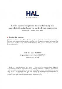
range of possible word-sequences in Eq. 2 was also limited to those in a lattice. To evaluate the performance of discriminative classifiers with large margin training, a range of model structures were compared. A consistent 12 dimensional feature-space ϕLL in Eq. 4, was used in this task. The baseline generative system was HMM based with VTS compensation. These compensated models were also used to derive the features for the discriminative models. The baseline results on test set A are shown in the HMM column of Table I. The first discriminative system built used the binary SVM combination schemes proposed in [7]. Here the observation sequences were segmented at the word-level based on the 1-best recognition output from the HMM system. A total of 66 SVMs were trained. During recognition, for each segmentation, 66 SVMs were evaluated. The results on set A are shown in the SVM column of Table I. The second system was the unstructured log-linear model with feature φ(O, w; λ) defined in Eq. 5. In this case the model trained in Eq. 15 degenerates to the multi-class SVMs (MSVM). Thus the results are shown in the column named MSVM. The same segmentation as the SVM system was used. For this system only a single model is trained. The final discriminative system was the structured ˆ λ) defined log-linear model (SLLM) with feature φ(O, w; θ, in Eq. 9 for continuous ASR. The results are in the SLLM column.1 Examining the results in Table I, the SLLM achieved the best results among all the systems under all the noise conditions. The difference in performance between the SLLM and MSVM systems shows the impact of using only the 1-best segmentation, as both systems effectively use the same joint feature-space. Restricting the segmentation degrades performance by about 6% relative. It is also interesting to compare the integrated multi-class SVM training (MSVM) with the binary SVM combination approach (SVM). The integrated training yielded a 9% reduction in error rate. The full results for all three test sets are shown in Table II. Compared to the MSVM performance, the SLLM provided 6%, 9% and 7% relative improvement for test set A, B and C. In addition to the systems evaluated in Table I, the stand alone binary SVM and SVM+HMM fusion rescoring described in [7] were examined. In these systems the ϕ∇ feature-space using only the two words being considered in the binary classification was used. This is a larger feature-space, specific to the binary classification task being considered. This gave a gain over ϕLL (O; λ) space. The performance of SLLM 1 Note that the number of parameters in HMM and proposed SLLM system are in the same range—more than 45, 000 for HMM and 144 more for SLLM.
Model HMM
Features —
Dim —
SVM ϕ∇ (O; λ) SVM+HMM ϕ∇ (O; λ) SVM ϕLL (O; λ) MSVM φ(O, w; λ) SLLM φ(O, w; θ, λ)
Param. λ
1500 αsvm , λ 1500 αsvm , λ, ² M αsvm , λ M2 α, λ M2 α, λ
Set A Set B Set C 9.84 9.11 9.53 7.95 7.52 9.10 8.27 7.78
8.05 7.35 8.68 8.06 7.31
8.64 8.11 9.25 8.64 8.02
TABLE II AVERAGE WER AMONG ALL NOISE CONDITIONS OF VTS BASED HMM, SVM, MSVM, SLLM (M = 12), AND SVM WITH HMM FUSION [7].
approach was comparable to the best fusion approach but with a more compact (144 dimensional) joint feature space which can be easily extended to large vocabulary systems. VI. C ONCLUSION This paper has proposed a structured log-linear model with a noise-robust joint feature space for continuous ASR. This model has a number of attractive features. First, it provides an elegant way of combining discriminative and generative models which allows noise-robust model compensations to be easily applied. Second, the model can capture joint information from the observations and labels. Third, the joint feature space can be decomposed at the arc level. This allows efficient decoding and training with lattices, which is important for any large vocabulary extensions. Fourth, the model can be trained under the large margin criterion. Depending on the nature of the joint feature-space and labels, this form of model is closely related to structured SVMs and Multi-class SVMs. Results on the AURORA 2 task demonstrate that modelling the structure information yields significant improvements. Currently the “most likely” alignment is given by Viterbi likelihood. Future work will examine optimizing the alignment θ with α during the training and decoding. R EFERENCES [1] D. Povey, “Discriminative training for large vocabulary speech recognition,” Ph.D. dissertation, Cambridge University, 2004. [2] F. Sha and L. K. Saul, “Large margin hidden markov models for automatic speech recognition,” in Neural Information Processing Systems. MIT Press, 2007, pp. 1249–1256. [3] G. Zweig and P. Nguyen, “A segmental CRF approach to large vocabulary continuous speech recognition,” in ASRU, 2009. [4] O. Birkenes, T. Matsui, and K. Tanabe, “Isolated-word recognition with penalized logistic regression machines,” in ICASSP 2006, vol. 1, 2006. [5] M. Layton and M. Gales, “Augmented statistical models for speech recognition,” in Proc. ICASSP, Toulouse, 2006. [6] N. Smith, “Using augmented statistical models and score spaces for classification,” Ph.D. dissertation, University of Cambridge, 2003. [7] M. J. F. Gales and F. Flego, “Discriminative classifiers with adaptive kernels for noise robust speech recognition,” Comput. Speech Lang., vol. 24, no. 4, pp. 648–662, 2010. [8] B. Taskar, “Learning structured prediction models: a large margin approach,” Ph.D. dissertation, CA, USA, 2005. [9] A. Acero, L. Deng, T. Kristjansson, and J. Zhang, “HMM Adaptation using Vector Taylor Series for Noisy Speech Recognition,” in Proc. ICSLP, Beijing, China, 2000. [10] I. Tsochantaridis, T. Joachims, T. Hofmann, and Y. Altun, “Large margin methods for structured and interdependent output variables,” J. Mach. Learn. Res., vol. 6, pp. 1453–1484, 2005. [11] K. Crammer, Y. Singer, N. Cristianini, J. Shawe, and B. Williamson, “On the algorithmic implementation of multiclass kernel-based vector machines,” J. Mach. Learn. Res., vol. 2, 2001. [12] H. Liao and M. Gales, “Joint uncertainty decoding for robust large vocabulary speech recognition,” Cambridge University, Tech. Rep. CUED/F-INFENG/TR552, November 2006. [13] S.-X. Zhang and M. J. F. Gales, “Structured log linear models for noise robust speech recognition,” Cambridge University, Tech. Rep. CUED/FINFENG/TR123, 2010, available from: http://mi.eng.cam.ac.uk/∼mjfg.