Studying neural selectivity for motion using high-field

Studying neural selectivity for motion using high-field fMRI Alex Beckett, MSc.

Thesis submitted to The University of Nottingham for the degree of Doctor of Philosophy February 2013

Abstract Functional magnetic resonance imaging (fMRI) offers a number of opportunities to non-invasively study the properties of the human visual system. Advances in scanner technology, particularly the development of high-field scanners, allow improvements in fMRI such as higher resolution and higher signal to noise ratio (SNR). We aimed to examine what these advances in scanner technology, combined with novel analysis techniques, can tell us about the processing of motion stimuli in the human visual cortex. In Chapter 3 we investigated whether high-resolution fMRI allows us to directly study motion-selective responses in MT+. We used event-related and adaptation methods to examine selectivity for coherent motion and selectivity for direction of motion, and examined the potential limitations of these techniques. One particular analysis technique that has been developed in recent years uses multivariate methods to classify patterns of activity from visual cortex. In Chapter 4 we investigated these methods for classifying direction of motion, particularly whether successful classification responses are based on fine-scale information such as the arrangement of direction-selective columns, or a global signal at a coarser scale. In Chapter 5 we investigated multivariate classification of non-translational motion (e.g. rotation) to see how this compared to the classification of translational motion. The processing of such stimuli have been suggested to be free from the large-scale signals that may be involved in other stimuli, and therefore a more powerful tool for studying the neural architecture of visual cortex. Chapter 6 investigated the processing of plaid motion stimuli, specifically ’pattern’ motion selectivity in MT+ as opposed to ’component’ motion selectivity. These experiments highlight the usefulness of multivariate methods even if the scale of the signal is unknown. Parts of the work discussed in Chapter 4 were published in the following article:

i

Beckett A, Peirce J, Sanchez-Panchuelo R, Francis S, & Schluppeck D ’Contribution of large scale biases in decoding of direction-of-motion from high-resolution fMRI data in human early visual cortex.’ NeuroImage 2012

ii

Acknowledgements Firstly, I would like to thank my supervisor Denis Schluppeck for first giving me the opportunity to work with fMRI, and for the extensive help and feedback he gave during the writing of this thesis. I would also like to thank Jon Peirce for his help and feedback for the work that went into this thesis. In addition I would like to thank Julien Beslie and Rosa Sanchez for their help with the methodology and data collection in these experiments. I would also like to thank the Nottingham Visual Neuroscience Group for providing such a great working environment. Finally, I would also like to offer a huge thank you to Molly Simmonite. I couldn’t have done this without her.

iii

Contents 1

Introduction

1

1.1

The Visual System . . . . . . . . . . . . . . . . . . . . . . . . . . . . . . . .

2

1.1.1

From Retina to Brain . . . . . . . . . . . . . . . . . . . . . . . . . .

2

1.1.2

V1 . . . . . . . . . . . . . . . . . . . . . . . . . . . . . . . . . . . . .

5

1.1.3

Visual Cortical Pathways . . . . . . . . . . . . . . . . . . . . . . .

8

1.1.4

Extrastriate Cortical Areas . . . . . . . . . . . . . . . . . . . . . . .

9

Magnetic Resonance Imaging . . . . . . . . . . . . . . . . . . . . . . . . .

15

1.2.1

Nuclear Magnetic Resonance . . . . . . . . . . . . . . . . . . . . .

15

1.2.2

Magnetic Resonance Imaging . . . . . . . . . . . . . . . . . . . . .

21

1.2.3

Functional MRI . . . . . . . . . . . . . . . . . . . . . . . . . . . . .

24

Experimental techniques . . . . . . . . . . . . . . . . . . . . . . . . . . . .

29

1.3.1

Adaptation . . . . . . . . . . . . . . . . . . . . . . . . . . . . . . .

29

1.3.2

MVPA . . . . . . . . . . . . . . . . . . . . . . . . . . . . . . . . . .

31

1.2

1.3

2

General Methods

36

2.1

Cortical Segmentation and Flattening . . . . . . . . . . . . . . . . . . . .

36

2.2

Retinotopic Mapping . . . . . . . . . . . . . . . . . . . . . . . . . . . . . .

40

2.2.1

Identifying visual areas . . . . . . . . . . . . . . . . . . . . . . . .

45

fMRI Methods . . . . . . . . . . . . . . . . . . . . . . . . . . . . . . . . . .

49

2.3.1

Participants . . . . . . . . . . . . . . . . . . . . . . . . . . . . . . .

49

2.3.2

Visual Stimuli . . . . . . . . . . . . . . . . . . . . . . . . . . . . . .

49

2.3.3

Functional Imaging . . . . . . . . . . . . . . . . . . . . . . . . . . .

49

2.3

iv

C ONTENTS

3

51

2.3.5

Data Analysis . . . . . . . . . . . . . . . . . . . . . . . . . . . . . .

51 58

3.1

Coherence Response Curves . . . . . . . . . . . . . . . . . . . . . . . . . .

59

3.1.1

Methods . . . . . . . . . . . . . . . . . . . . . . . . . . . . . . . . .

61

3.1.2

Results & Discussion . . . . . . . . . . . . . . . . . . . . . . . . . .

62

Adaptation . . . . . . . . . . . . . . . . . . . . . . . . . . . . . . . . . . . .

65

3.2.1

Methods . . . . . . . . . . . . . . . . . . . . . . . . . . . . . . . . .

67

3.2.2

Data Analysis . . . . . . . . . . . . . . . . . . . . . . . . . . . . . .

67

3.2.3

Results & Discussion . . . . . . . . . . . . . . . . . . . . . . . . . .

67

General Discussion . . . . . . . . . . . . . . . . . . . . . . . . . . . . . . .

70

3.3

Classification of Motion Direction

72

4.1

Classification with High Field fMRI . . . . . . . . . . . . . . . . . . . . .

72

4.1.1

Methods . . . . . . . . . . . . . . . . . . . . . . . . . . . . . . . . .

79

4.1.2

Results . . . . . . . . . . . . . . . . . . . . . . . . . . . . . . . . . .

80

4.1.3

Discussion . . . . . . . . . . . . . . . . . . . . . . . . . . . . . . . .

86

Investigating the contribution of radial bias . . . . . . . . . . . . . . . . .

92

4.2.1

Methods . . . . . . . . . . . . . . . . . . . . . . . . . . . . . . . . .

92

4.2.2

Results . . . . . . . . . . . . . . . . . . . . . . . . . . . . . . . . . .

93

4.2.3

Discussion . . . . . . . . . . . . . . . . . . . . . . . . . . . . . . . .

96

4.2

4.3

4.4 5

Attention Control Task . . . . . . . . . . . . . . . . . . . . . . . . .

Pilot Experiments: Direction Selectivity in MT+

3.2

4

2.3.4

Controlling for Eye Movements . . . . . . . . . . . . . . . . . . . . . . . . 100 4.3.1

Methods . . . . . . . . . . . . . . . . . . . . . . . . . . . . . . . . . 100

4.3.2

Results and Discussion . . . . . . . . . . . . . . . . . . . . . . . . . 100

4.3.3

Discussion . . . . . . . . . . . . . . . . . . . . . . . . . . . . . . . . 101

General Discussion . . . . . . . . . . . . . . . . . . . . . . . . . . . . . . . 103

Classification of non-translational motion 5.1

105

Classification of rotation and ’spiral’ motion . . . . . . . . . . . . . . . . 105 5.1.1

Methods . . . . . . . . . . . . . . . . . . . . . . . . . . . . . . . . . 106

v

C ONTENTS

6

Results . . . . . . . . . . . . . . . . . . . . . . . . . . . . . . . . . . 108

5.1.3

Discussion . . . . . . . . . . . . . . . . . . . . . . . . . . . . . . . . 111

Classification of Pattern Motion 6.1

6.2

6.3 7

5.1.2

115

Grating to Plaid Classification . . . . . . . . . . . . . . . . . . . . . . . . . 121 6.1.1

Methods . . . . . . . . . . . . . . . . . . . . . . . . . . . . . . . . . 121

6.1.2

Results . . . . . . . . . . . . . . . . . . . . . . . . . . . . . . . . . . 124

6.1.3

Discussion . . . . . . . . . . . . . . . . . . . . . . . . . . . . . . . . 131

Dot to Paired Dot Classification . . . . . . . . . . . . . . . . . . . . . . . . 135 6.2.1

Methods . . . . . . . . . . . . . . . . . . . . . . . . . . . . . . . . . 137

6.2.2

Results & Discussion . . . . . . . . . . . . . . . . . . . . . . . . . . 138

General Discussion . . . . . . . . . . . . . . . . . . . . . . . . . . . . . . . 140

General Discussion

142

References

150

vi

Chapter 1

Introduction The human visual system takes in a huge amount of raw information, in the form of patterns of light hitting the back of the eye, and extracts from this useful information about our surroundings. Understanding the process by which this analysis is performed has been a key aim of psychology and neuroscience since their inception. Among the tools available to psychologists and neuroscientists are behavioural experiments with psychophysics and visual illusions, examining the neuropsychological effects of brain damage on vision, and measuring the activity of single cells in animals in response to visual stimuli. The recent development of non-invasive techniques for measuring and analysing neural information has been key in understanding how the visual system ultimately transforms the patterns of light entering the eye into a neural signal that allows us to understand and interact with the world around us. The most consistently used neuroimaging technique for human volunteers has been Functional Magnetic Resonance Imaging (fMRI), with a huge increase in the number of published papers using the technique since its development in the early 1990’s (Ogawa et al., 1990). In this thesis I will examine what recent technical developments in this field can tell us about the analysis of visual motion information in the human visual cortex. FMRI has allowed studies of the processing performed in each stage of the human visual system to be related to evidence from electro-physiology in animals, neuropsychological studies of human subjects after brain damage, and behavioural studies in healthy subjects. The following sections summarise the current literature on the function of the visual system, and how the evidence from different research methods complement and differ from one another.

1

C HAPTER 1: I NTRODUCTION

1.1

The Visual System

The processing of visual information begins with light entering the eye via the pupil and hitting the retina on the back of the eye, and continues on through the visual cortex and beyond. In the following sections I will briefly summarise the pathway from the retina to the visual cortex, and examine the different aspects of analysis at each stage.

1.1.1

From Retina to Brain

The initial stage of processing for visual information occurs when light falls on the retina, the array of photoreceptors on the back of eye, having been focussed (and inverted) by the lens of the eye. In vertebrates, the output of these photoreceptors is collected and combined by retinal ganglion cells, with a large amount of processing being done at this initial stage (Callaway, 2005; Lettvin et al., 1959). Whilst the photoreceptors in the retina simply change their level of response depending on the light that falls on them, the retinal ganglion cells are more selective in their responses. It is worth noting that a significant amount of processing is done at the very first level of processing in the retina, and important information about a visual scene is extracted at this very early stage, well before the visual cortex itself (although the details of this are beyond the scope of this thesis). The area of retina (and hence visual field) which will cause a retinal ganglion cell to fire if stimulated is called the ’receptive field’ (RF) for that cell, and many retinal ganglion cells in vertebrates, for examples those in the cat retina, have a ’centre-surround’ RF arrangement, with a central region that either excites or inhibits the cell in response to light, and surrounding ring with the opposite sensitivity (Kuffler, 1953). Light falling across the whole RF will cause the cell to fire very weakly, whereas light falling only on the excitatory centre (if the cell is ’on-centre’) will cause the cell to fire rapidly (if the cell is ’off-centre’, light falling on the surround only will cause rapid cell firing). Therefore these cells are sensitive to contrast, discontinuities in the distribution of light corresponding to edges, rather than simply to different levels of illumination. The axons of the majority of retinal ganglion cells project to the brain along the optic nerves. The optic nerves from each eye meet at the optic chiasm (Figure 1.1), where the information is combined and split depending on its origin on the retina. Fibres originating from the nasal part of the retina cross over to the other side of the brain, whilst fibres originating at the temporal side of the retina continue on the same side. The result of this decussation is to split the visual field into a left and right portion, with the left visual field (from both eyes) being processed by the right side of the brain and 2


Figure 1.1: A diagram indicating the path taken by visual information from the eye to the visual cortex, indicating how the visual field is represented at each stage in each cortical hemisphere. Adapted from Netter (2010)

3

C HAPTER 1: I NTRODUCTION the right visual field being processed by the left side of the brain (Figure 1.1). Following the optic chiasm, the optic nerve is referred to as the optic tract. The majority of the fibres which make up the optic tract terminate at the Lateral Geniculate Nucleus (LGN) in the thalamus (Figure 1.1); the rest terminate in the midbrain, primarily at the Superior Colliculus, as well as the suprachiasmatic nucleus. In many primates, including humans, the LGN is subdivided into a number of layers, with different layers receiving input from different populations of retinal cells, with preferences for different kinds of stimuli (Wiesel and Hubel, 1966). In addition, each layer receives input from only one eye. The uppermost layers, known as parvocelluar layers, receive input from a class of cells known as midget retinal ganglion cells whilst the bottom layers, the magnocellular layers, receive input from parasol cells. These retinal ganglion cells have different receptive field properties, and these two kinds of layers form the beginning of two segregated visual pathways that continue through the visual system (Livingstone and Hubel, 1988). The two visual streams process different kinds of stimuli, with the parvocellular (P) pathway favouring high spatial frequency and colour information, and the magnocellular (M) pathway carrying coarser spatial frequency and motion information. Cells in between the magno- and parvocellular layers receive input from bistratified retinal ganglion cells and represent a third processing stream, the koniocellular stream, whose perceptual specialization is unclear at this point. Each layer of the LGN contains a full representation of the contralateral visual field (Figure 1.1), and axons projecting from neighbouring parts of the retina terminate at neighbouring geniculate cells, creating an ordered map of the retina. This representation that preserves the topography of the retina is known as a retinotopic map, and is a feature of many mammalian brains. The layers of the LGN are arranged in such a way that the retinotopic maps of each layer are aligned. The receptive fields of neurons in mammalian LGN closely resemble those of retinal ganglion cells in terms of on-off surround (Hubel and Wiesel, 1961). Although the exact function of the LGN is still debated (Callaway, 2005), its separation of signals from the retina in terms of function and origin is believed to set-up a similar segregation in visual cortex. The LGN projects to both the visual cortex and additionally to the superior colliculus, a nucleus involved with the control of eye movements. The LGN projects to the cortex via the optic radiation, which terminates in layer 4 of the primary visual cortex (V1). The retinotopic representation established in the LGN is maintained in V1: different areas of the contralateral visual field are mapped in an orderly fashion in area V1 of each cortical hemisphere, with adjacent points in the visual field being processed by adjacent neurons in cortex (Figure 1.1). One key feature

4

C HAPTER 1: I NTRODUCTION of the retinotopic map that is present at the LGN and emphasised in visual cortex is that the fovea tends to be overrepresented compared to the periphery of the retina, with larger receptive fields in the periphery and smaller at the fovea. This property is known as cortical magnification. Retinotopic organization persists in many visual areas beyond V1, and this feature is exploited in identifying and defining visual areas with fMRI in individual subjects. A full discussion of the methodology for retinotopic mapping is given in section 2.2.

1.1.2

V1

V1 lies in the calcarine sulcus at the posterior pole of the occipital cortex (Figure 1.1). V1 has a well defined representation of the contralateral visual field, organised retinotopically, with adjacent points of the visual field represented at adjacent locations on the cortical surface. As with ganglion cells in the retina, cortical cells do not simply respond to levels of contrast, but are selective for certain properties of an image. The properties of V1 cells were first extensively studied in animals by Hubel and Wiesel (1959, 1963, 1969). One key finding was that a population of cells in cat primary visual cortex, which they named ’simple cells’, would show preferential activity for bars of light oriented at a specific angle. This selectivity is due to the shape of the cells’ receptive fields, which have elongated On and Off regions with a given orientation (Hubel and Wiesel, 1959). These cells will only fire when the dark and light portions of an oriented bar fall exactly on the correct regions, making them highly selective for position and orientation. A second class of cells, called ’complex cells’ by Hubel and Wiesel (1962) has the same selectivity for orientation, but their receptive fields do not have as defined On/Off regions as simple cells, so they respond to a properly oriented stimulus falling anywhere in its receptive field. A third class of cells, known as hypercomplex or ’end-stopped’ cells, are sensitive to the length of a stimulus as well as its orientation, and will reduce their response if the stimulus exceeds the length of the receptive field (Hubel and Wiesel, 1965). These sub-classes of visual cells have also been demonstrated in non-human primates (Hubel and Wiesel, 1968). A further finding by Hubel and Wiesel (1959) was that cells with the same orientation selectivity were grouped together perpendicular to the cortical surface, leading to the development of the idea of ’orientation columns’ in primary visual cortex. Cortical columns were initially identified in somatosensory cortex of the cat (Mountcastle et al., 1957), where cells perpendicular to the cortical surface had sensitivity to the same kind of tactile stimulation. Hubel and Wiesel (1959) found that the preferred orientation of cells in cat visual cortex was constant as the recording electrode was pushed perpen5


Figure 1.2: Orientation Columns (A) and ODCs (B) measured from primate V1 using optical imaging. Colour coding in A indicates preferred orientation (horizontal = blue, 45 = red, vertical = yellow, 135 = green). Colour coding in B indicates preference for stimulated eye (dark = left eye, light = right eye). Dark lines in both figures indicate borders between ODCs, thin-lines indicate iso-orientation contours. The two dimensions can be seen to run broadly orthogonal to each other. Taken from Ts’o et al. (2009)

dicularly through the cortical surface, but varied regularly as the electrode progressed obliquely. Similar results were found in macaque visual cortex (Hubel and Wiesel, 1974), leading to the formulation of a model of orientation ’slabs’ arranged across the cortical surface, with adjacent slabs having slightly shifted orientation preferences. Hubel and Wiesel (1974) coined the term ’hypercolumn’ to describe an area of cortex containing a set of columns with the full range of orientation preferences. As well as preferences for stimulus orientation, Hubel and Wiesel (1962, 1969) also showed that cells in visual cortex of cats and macaques have a preference for stimulation through one eye versus the other, and that cells with similar eye preference are also arranged on the cortical surface into ’Ocular Dominance Columns’ (ODCs). These two observations led to the development of what came to be known as the ’ice-cube’ model, with hypercolumns for orientation and ODCs orthogonal to each other on the cortical surface, with any given area of cortex containing multiple, overlapping columns (Hubel and Wiesel, 1977), hence containing cells tuned across a complete range of values for each domain. This block of tissue was referred to as a ’module’, and set forth the idea that these discrete units were responsible for analysing the visual field fully across these domains at a given retinotopic location. Further evidence of an ordered arrangement of selective neurons came from optical imaging, which uses the light reflected from an exposed cortical surface to measure neural activity. This allows the preferences of a large number of cells in the visual cor6


Figure 1.3: Example of a simple cell in cat visual cortex with orientation (left) and spatial frequency (right) tuning, demonstrating the bell shaped tuning curve in both instances. Adapted from Webster and De Valois (1985)

tex to be measured simultaneously, and allows the direct visualization of the layout of neuronal preference maps on the cortical surface (Figure 1.2). Whilst several studies indicated that orderly arrangement of cells with similar preferences for orientation and stimulated eye existed in cat and primate visual cortex and were broadly orthogonal (Grinvald et al., 1986; Ts’o et al., 2009), some revision of the Hubel and Wiesel (1977) model was necessary. For example the addition of ’pin-wheel’ arrangement of preferred orientation (Bonhoeffer and Grinvald, 1991), where the preferred orientation of the cells progressed radially around a centre point instead of along the cortical surface (although some have argued that this feature of orientation maps from optical imaging is simply an artefact caused by draining veins). The concept of a ’hypercolumn’ however has been more elusive, with a periodic repetition of a ’module’ containing neural mechanisms for a full analysis of visual space often difficult to establish (Bartfeld and Grinvald, 1992). In humans, the existence of columns was initially demonstrated using post-mortem cytochrome oxidase (CO) tissue staining (which stains cells based on their metabolic activity) in the visual cortex of patients with monocular vision loss, leaving ODCs for the missing eye lighter than those for the healthy eye (Adams et al., 2007). Recently, the existence of ODCs and orientation columns in human V1 has been demonstrated non-invasively using high-resolution fMRI at 7T (Yacoub et al., 2007, 2008). Cells in V1 also display preferences for additional stimulus properties, for example spatial frequency (relating to the level of detail in an image) (Campbell et al., 1969;

7

C HAPTER 1: I NTRODUCTION De Valois et al., 1982a). Cortical neurons demonstrate selectivity for both a given orientation and a given spatial frequency, generally showing a bell shaped tuning curve to both properties (Figure 1.3). Neurons such as this can be thought of a acting as a set of spatial frequency filters at different orientations, essentially performing a crude form of Fourier analysis of an image. Whilst columnar architecture for orientation has been demonstrated in both animals (Hubel and Wiesel, 1962, 1974) and humans (Yacoub et al., 2008), an ordered representation for spatial frequency has not been. A subset of cells in cat and monkey V1 have been shown to be selective for direction of motion as well as orientation (De Valois et al., 1982b; Hubel and Wiesel, 1962), in that neurons increase their activity for a contour of their preferred orientation moving in a given direction of motion. An ordered map of direction preference, as for orientation, has been demonstrated in early visual cortex for some animals (Welicky et al., 1996), although not in primate V1 (Lu et al., 2010) where only axis of direction columns could be demonstrated. Cells in V1 with motion selectivity primarily project to areas thought to be involved in motion processing, such as area MT/V5 , both directly and via areas such as V2 and V3 (Maunsell and van Essen, 1983).

1.1.3

Visual Cortical Pathways

V1 projects directly to a number of other visual areas, as well as indirectly to a number of others via V2. One key feature of these cortical projections is a segregation into two visual pathways. The majority of connections from V1 (via V2 and V4) project ventrally towards the temporal lobe, and are primarily made up of projections from the P pathway in the LGN. The remainder of connections project dorsally towards the parietal lobe, and are primarily of the M pathway. This continues the two visual streams established at the LGN, and suggests that these two streams have distinct functions based on the specialization for form and motion in the two pathways (Livingstone and Hubel, 1988). Although the segregation between magnocellular and parvocellular projections in the two streams may not be absolute (Maunsell et al., 1990), the idea of two cortical streams specialized for different aspects of visual processing has also been supported by electrophysiology and lesion studies. Ungerleider and Mishkin (1982) named these two projections the dorsal and ventral streams based on the direction of their projections from V1, and from work with macaque lesions hypothesised the dorsal stream as the ’where’ pathway, concerned with spatial awareness, and the ventral stream as the ’what’ pathway, dealing with the recognition of objects. Evidence for such an interpretation comes from a ’double dissociation’ in human studies after brain damage, with lesions of posterior parietal cortex leading 8


Figure 1.4: Representations of the visual field (Top Right) in the visual cortex of human (A) and macaque (B). Representations of cortex not to scale. Ventral V1-3 contain representations of the contralateral Upper Visual Field (UVF), dorsal V1-3 contain representations of the contralateral lower visual field (LVF). Some areas beyond contain a representation of the full contralateral visual field. Figure taken from Larsson and Heeger (2006).

to optic ataxia (a disorder involving failures of hand-eye coordination), and lesions of ventral visual areas leading to visual agnosia (an impairment of recognition of visually presented objects) ( see Milner and Goodale (2008) for a review). Goodale and Milner (1992) presented the split in terms of ’vision for action’ in the dorsal stream, and ’vision for perception’ in the ventral stream. The independence and separation of the dorsal and ventral streams has been questioned in recent years (Schenk and McIntosh, 2010), and the picture emerging seems to be of a relative rather than an absolute specialization for different aspects of vision, with a large amount of interaction between the areas. However, the two streams hypothesis provides a useful framework to consider the different types of processing done in each visual area.

1.1.4

Extrastriate Cortical Areas

The extrastriate areas that V1 projects to (both indirectly and directly) are defined by having an ordered retinoptopic mapping, preserving the orderly representation that exists in LGN and V1 (Figure 1.4). Receptive fields in these area also tend to be larger 9

C HAPTER 1: I NTRODUCTION than those in V1. In addition, some extrastriate areas have been shown to demonstrate a preference for specific kinds of visual processing. The next section reviews some of the evidence of the different functional properties of these areas.

V2 Area V2 in each hemisphere comprises two areas, dorsal and ventral of V1 respectively, each with a map of a quadrant of the contralateral visual field (Figure 1.4). V2 receives strong connections from V1, as well as sending many feedback connections to this area. V2 also projects to areas V3, V4, and V5/MT. Cells in V2 show many tuning properties similar to V1 cells such as orientation, spatial frequency and binocular disparity (Levitt et al., 1994). In addition, V2 cells also have additional properties such as tuning for relative disparity (Thomas et al., 2002) and tuning for more complex interactions of orientations (Hegdé and Van Essen, 2000). This suggests that V2 is responsible for building upon the simple visual processing undertaken in V1 to allow more complex processing. Lesions of this area in the macaque affect performance in complex spatial tasks with no effect on acuity or contrast sensitivity (Merigan et al., 1993). It has been demonstrated that tuning for disparity follows a columnar arrangement in macaque V2, orthogonal to one for orientation (Ts’o et al., 2009). V2 has a striped organization, with different stripes known as thick, thin and pale depending on their appearance after staining with cytochrome oxidase (Livingstone and Hubel, 1984), and it has been suggested that the different stripes contain cells with functionally distinct properties; for disparity and orientation in the thick stripes, colour in the thin stripe and orientation in the pale stripes (Roe and Ts’o, 1995). This suggests the mechanisms for a full analysis of a point in visual space are more distributed and segregated over a patch of cortex in V2 (Ts’o et al., 2009), compared to V1, where hypercolumns for OD and orientation are expected to overlap and interact. Additionally to the organization for orientation and disparity, a map for preferred direction running orthogonally to preferred orientation has been demonstrated in the thick stripes of macaque V2 (Lu et al., 2010), which are known to project to direction selective areas such as MT and V3A.

V3 An area known as V3 lies anterior of V2 on both dorsally and ventrally (Figure 1.4), which receives input from V1 and V2 and projects to V4 and MT. The exact makeup of this area, including how many areas it is subdivided into and their functional prop10

C HAPTER 1: I NTRODUCTION erties, is still a matter of debate (see Lyon and Connolly (2012) for a recent review). V3 neurons in macaque show tuning for orientation (although broader than the tuning seen in V2), a large proportion show direction selectivity (with some evidence of pattern selectivity) and some evidence for colour selectivity (Gegenfurtner et al., 1997). The dorsal part of V3 contains a representation of the lower visual field only, and the corresponding ventral area containing the upper field is sometimes considered as a separate area known as Ventral Posterior (VP) (Burkhalter and Van Essen, 1986), with selectivity for motion and colour split between the two areas. The extent to which this ventral area is functionally distinct from V3 is still controversial (Lyon and Connolly, 2012; Zeki, 2003). For the purposes of this thesis, the areas bordering V2 that together contain a complete representation of the contralateral visual field were treated as a single visual area. In macaques, an additional dorsal visual area beyond V3 and separate from V4 was identified on the basis of its retinotopic map, and was named the V3 Accessory area (subsequently known as V3A) (Van Essen and Zeki, 1978). V3A was subsequently shown to be an entirely separate area to V3, although the V3A name was kept (Tootell et al., 1997). One key feature of macaque V3A is that it contains a full representation of both the upper and lower parts of the contralateral visual field, unlike other nearby areas (Van Essen and Zeki, 1978) (Figure 1.4). Macaque V3 was shown to be highly direction and motion selective, whereas macaque V3A was shown to be much less so. An area beyond human dorsal V3 was also identified on the basis of its retinotopy, and was also referred to as V3A owing to the similarity of its location to macaque V3 (Tootell et al., 1997). However, in humans the function of the two areas appear to be reversed, in that V3A shows greater motion and direction selectivity than V3 in fMRI experiments (Tootell et al., 1997). An additional area lateral to human V3A was also identified, containing a full representation of the contralateral visual field and sharing a foveal confluence with V3A separate from that of V1-V3, known as V3B (Smith et al., 1998) (Figure 1.4). The exact function of human V3B is unclear at this point, although it appears to be involved in processing shape information (Zeki, 2003), and it is frequently considered as a single Region of Interest (ROI) combined with V3A. Beyond V3A/B, an addition representation of the contralateral hemifield exists in humans in an area known as V7 (Tootell et al., 1998) (Figure 1.4), although the function of this area is unclear.

11


V4 In the macaque, V4 lies anterior to V3, and contains a full representation of the contralateral visual field, with the upper and lower quadrants in the ventral and dorsal sections respectively (Figure 1.4). V4 receives input from V2 and V1, as well as regions of temporal cortex and areas within the dorsal stream. V4 was initially suggested as a specialized area for colour processing (Zeki, 1983), based on colour (rather than wavelength) selective receptive fields, with some evidence of a columnar organisation for colour. This specialization for colour was contrasted against the apparent specialization for motion in area MT, suggesting the modularity of processing for different aspects of vision. Studies also demonstrated selectivity for orientation in a majority of V4 neurons, with some evidence that cells in V4 could only be optimally driven using more complex stimuli than the sinusoidal gratings used in studying earlier areas such as V1 (Desimone and Schein, 1987). Lesions of macaque V4 showed slight deficits in certain detection and discrimination tasks, as well as more severe deficits in tasks involving the discrimination of form (Merigan, 1996), suggesting a broader role for this area than simply being the ’colour’ area of cortex. The human homologue of macaque V4 has been difficult to ascertain. One key area of debate has been whether the visual hemifield representation is split dorsally and ventrally, or whether a complete hemifield representation exists within ventral V4, and no dorsal V4 exists in humans (Tootell and Hadjikhani, 2001). Lesions of ventral cortex in humans can lead to achromatopsia (deficit in colour vision) (Zeki, 1990), and perceptual deficits similar to those seen in monkeys, suggesting that the human homologue of macaque area V4 lies in this part of cortex.

V5/MT and MST It has been suggested that some areas in extrastriate cortex, specifically dorsal/parietal areas, are specialized for motion processing. Direction-selective cells in monkey V1 project to an area of the superior temporal sulcus (STS) known as the middle temporal area (MT), which is itself heavily direction selective (Albright et al., 1984; Dubner and Zeki, 1971; Zeki, 1980). This area, known as either MT or V5 was suggested as an example of a specialized area for motion processing (Zeki, 1974), due to its strong direction selectivity and apparent nonselectivity for other visual properties such as colour. Additionally, lesions of V5/MT of the macaque elevate direction-detection thresholds without affecting contrast detection thresholds (Newsome and Pare, 1988). Area V5 receives inputs from V1, V2, dorsal V3, LGN and the pulvinar, with the vast 12

C HAPTER 1: I NTRODUCTION majority of its input coming from layer 4B of V1, which is know to have a higher proportion of direction-selective cells compared to other layers (Maunsell and van Essen, 1983). Direction-selective responses in V5/MT persist after inactivation of V1, indicating a role for sub-cortical inputs in direction selectivity, with residual direction selectivity removed by inactivation of the SC (Gross, 1991). MT has also been suggested to be a key part of the dorsal cortical processing stream (Ungerleider and Mishkin, 1982), and projects to a number of areas in posterior parietal cortex. It also projects to areas known to be sensitive to optic flow (MST) and for controlling eye movements (Frontal Eye Fields). Similar to earlier visual areas, V5 is also retinotopically organized, containing a full representation of the contralateral hemifield (Van Essen et al., 1981) (Figure 1.4 B). Columns for preferred direction have been demonstrated in macaque MT (Albright et al., 1984; Dubner and Zeki, 1971), with smooth changes in preferred direction across successively sampled cells by the penetrating electrode, punctuated by sudden jumps in preference of 180 degrees. These findings suggested that columns of a given preference sit side by side with columns with the opposite preference, with these co-arranged units responding to opposite directions of motion referred to as axis of motion columns (Albright et al., 1984; Diogo et al., 2003). In addition, a columnar organisation for binocular disparity has been demonstrated in macaque MT (DeAngelis and Newsome, 1999), coexisting with the columnar arrangement for direction. Clustering for speed tuning has also been shown, though not with a columnar arrangement. Combined electrophysiological and behavioural work in primates indicates that activity in V5 is linked to the perception of motion: activity in this area predicts perceived direction and stimulation biases perceived direction toward the stimulated direction (Salzman et al., 1992). Although the proportion of direction selective cells in MT/V5 is higher than earlier visual areas, their tuning for direction, speed and disparity does not differ greatly from cells in V1 that project to this area (Movshon and Newsome, 1996). One way in which MT cells are differentiated from direction selective cells in V1 is by their larger receptive fields, leading to suggestions that MT neurons may allow motion be detected over larger displacements, mirroring the difference between ’long-range’ and ’short-range’ motion processes suggested by psychophysics (Mikami et al., 1986). However, the upper limits of spatial displacement that MT cells are sensitive to are similar to those in V1, despite the much larger RFs in MT (Churchland et al., 2005). An additional suggestion for the functional role of MT is that it is instrumental in computing the motion of whole objects, contrasted with a focus on local motion computation in earlier areas such as V1. A large proportion of cells in MT/V5 are selective for pattern direction,

13

C HAPTER 1: I NTRODUCTION rather than component direction (Movshon et al., 1985). For example, for a drifting plaid stimulus formed from two drifting gratings, component selective cells will respond to whichever grating more closely matches their preferred orientation, whilst a pattern selective cell will respond to the motion of the plaid itself, regardless of the underlying components. A number of additional areas sensitive to visual motion lie within the STS, including the medial superior temporal (MST) area and the floor of the STS (FST) (Desimone and Ungerleider, 1986). MST shares a number of properties with MT, such as a high proportion of direction selective neurons and link between activity in this area and the perception of motion (Celebrini and Newsome, 1994). The retinotopic organization in MST is much coarser than that seen in MT, and cells in this area tend to have much larger RFs that often extend into the ipsilateral visual hemifield (Desimone and Ungerleider, 1986). Additional functional differences also exist between the two areas, with many MST neurons shown to be selective for certain complex optic flow motions such as expansion, contraction and rotation, making them candidates for the processing of self-motion (Saito et al., 1986). The human homologue of V5/MT was first localised by the finding of patients with akinetopsia (’motion blindness’) after brain damage to temperoparietal areas, suggesting motion specialized areas in human visual cortex (Zihl et al., 1983). Subsequent fMRI studies found a strong response to moving compared to stationary stimuli around this area (Watson et al., 1993) , suggesting that it is the homologue of macaque area MT. The area of brain activated by motion is also believed to contain the homologues of a number of motion sensitive areas beyond MT (such as MST), so is referred to as MT+. The human homologue of MT (hMT) itself can be identified as the subsection of MT+ that contains a retinotopic map for the contralateral hemifield, and that responds only to motion in the contralateral hemifield (Huk et al., 2002), with an adjacent area showing ipsilateral responses designated as the human homologue of MST (hMST). Axis of motion columns, but not direction of motion columns, have also been demonstrated using high-resolution fMRI in hMT (Zimmermann et al., 2011).

14


1.2

Magnetic Resonance Imaging

Functional Magnetic Resonance Imaging (fMRI) is non-invasive method of measuring neural activity, with a high spatial resolution. fMRI can be considered a 4D version of anatomical MRI, which can form an image of the brain based on the properties of the underlying tissue when placed in a strong magnetic field. The following section provides an overview of the physics of generating an MR image, what these images tell us about the brain, and how 4D fMRI images (or a timeseries of 3D images) can be related to brain activity.

1.2.1

Nuclear Magnetic Resonance

Magnetic Resonance Imaging (and its functional form), relies on the properties of nuclei and their interactions with magnetic fields. Nuclear Magnetic Resonance (NMR) is the study of nuclei under the influence of a magnetic field. Certain kinds of atomic nuclei will behave in a predictable way when placed within a magnetic field, and this behaviour, and especially their behaviour when perturbed by an electromagnetic pulse, can tell us about the underlying tissue those atomic nuclei are a part of.

Nuclei and Spins In order to be studied with NMR, atomic nuclei must have a non-zero ’spin’, an intrinsic quantum property determined by spin quantum number S. Nuclei with an odd number of protons/neutrons, for instance Hydrogen atoms consisting of a single proton, have a non-zero S. This property gives these nuclei an angular momentum (J), and if a nucleus has spin then it will also possess a magnetic moment (µ) due to the inherent charge of the nucleus. Both of these forces can be represented as vectors with the same direction, related by the scalar factor g, the gyromagnetic ratio:

µ = g.J

(1.2.1)

This scalar factor g is the ratio between the charge and mass of a given spin. The gyromagnetic ratio is constant for a given nucleus of an isotope with spin, which is key in allowing the development of Magnetic Resonance images. The most abundant and biologically relevant example of a nucleus with spin is hydrogen, which due to its abundance in the human body is most commonly studied in MRI. Hence hydrogen nuclei will be used in subsequent discussion of spins.

15


A

B0

B B0 M

Figure 1.5: Atomic nuclei in a magnetic field. Left panel shows a spin in a parallel state, precessing around B0 . Right panel shows a number of spins aligned either parallel or anti-parallel with B0 . At equilibrium, a greater proportion are aligned parallel with B0 , creating the net magnetization vector M parallel with the external field.

If a large number of spins share a spatial location, their magnetic moments sum together to form a net magnetization vector (M). In the absence of a strong external magnetic field, the orientations of the axes of the individual spins will be distributed randomly, so will cancel each other out and lead to a very small M. However, when placed in a strong magnetic field (known as B0 in the case of an MRI scanner), the µ of each spin will experience a turning force trying to align it to the external magnetic field (Figure 1.5). In a steady state the spins do not align exactly with the external magnetic field, but due to their own inherent spin precess around an axis aligned to the external field in a gyroscopic motion. The frequency with which they precess around this axis is defined by the Larmor equation:

w = g.B

(1.2.2)

The frequency of precession is therefore know as the Larmor frequency (w), and is unique for each isotope due to its relation to the gyromagnetic ratio. Because of the spin quality of each system, the spins will align either parallel or antiparallel with the external field (Figure 1.5). The two alignment states have different energy states, low for parallel and high for anti-parallel, and it requires application of energy to cause a transition from the low- to high-energy state. This energy can be provided by the environment a spin is in, leading to a mix of up and down states in a population of spins. Generally there will be more spins in the parallel (low-energy) 16

C HAPTER 1: I NTRODUCTION state than the anti-parallel (high-energy) state, yielding a small (M) vector parallel with B0 . This magnetisation represents the signal available for NMR. The more spins there are in parallel, the larger M will be. The proportion of parallel spins, and hence M, can be increased by either decreasing the temperature of the spin system (removing the energy from the environment), or increasing the strength of the magnetic field. The net magnetization M can be thought of as a vector with two components, a longitudinal component Mz that is parallel/anti-parallel to B0 , and a transverse component Mxy that is perpendicular to the main magnetic field.

Radiofrequency Pulse The net magnetisation vector M is not directly measurable under equilibrium conditions because of the huge difference in strength between it and the external magnetic field vector B0 (B0

M). To overcome this the equilibrium state is perturbed, which

is achieved by applying a radio-frequency (RF) pulse at the Larmor frequency (w) of the spins. The RF pulse can be thought of as an oscillating magnetic field (B1 ), and although it is much smaller in magnitude than B0 , it can change the state of the spins in M if it is resonant with the precession frequency of those spins. The application of B1 causes the the proportion of spins in the low and high energy states to change from that at equilibrium, with more spins entering the high energy state. The application of B1 also causes the phases of the spins to align. This can be thought of as ’tipping’ the magnetic vector from its alignment with B0 along the z-axis. The actual motion of M is a complex spiral motion that is a combination of tipping into the xy plane and precessing around the z-axis, known as nutation. Because both B1 and M rotate around the z-axis at the Larmor frequency, it is often simpler to conceive the action of the B1 in a rotating frame of reference, which is achieved by changing the coordinate system from the ’laboratory frame’ ( x, y, z) to a frame of reference rotating at the Larmor frequency known as the ’rotating frame’ ( x 0 , y0 , z0 ) Figure (1.6). The z and z0 axis are the same in both coordinate systems. In the rotating frame, B1 appears as a stationary vector along x 0 , and M can be considered as simply ’tipping’ from the z0 axis towards the xy0 plane. An RF pulse is described by the angle it ’flips’ the M vector from the z0 axis towards the xy0 plane, known as the flip-angle a. The flip-angle is determined by the length of time that the RF pulse is applied. For example a 90 RF pulse will tip the M entirely into the xy0 plane, by causing all the spins to be in phase with no net difference between the number of spins in the ’up’ and down’ state, leading to a net magnetization in the xy0 plane. A spin perturbed from equilibrium by a 90 RF pulse is said to be ’saturated’ or ’excited’. 17


A

B

M

M B1

Figure 1.6: The effect of the RF pulse in the laboratory frame (A) and the rotating frame (B). A) In the laboratory frame, the application of the RF pulse tips the magnetization vector M into the xy plane as it spirals around the z axis (nutation). B) In the rotating frame, M remains stationary, and simply tips into the xy plane.

Relaxation The result of a 90 RF pulse is a net magnetisation precessing in the xy0 plane (due to the net-phase caused by the phase coherence of the spins in the system), and nonequilibrium magnetisation in the z0 direction caused by a change in the number of spins in the up and down states. Once the RF pulse is switched off the nuclei that contribute to M return to their initial equilibrium state, with a net magnetisation in the z0 direction and no coherence amongst the spins, through a process known as relaxation. During relaxation, M returns to alignment with z0 from being tipped into or through the xy0 plane, and the two component vectors return to their equilibrium state. During relaxation, the transverse Mxy component decays to 0, and the longitudinal Mz component returns to its equilibrium value. The rates of relaxation for the two components are determined by two time constants, which differ from tissue to tissue.

Longitudinal Relaxation (T1 ) Following the termination of the RF pulse, the spins placed in the anti-parallel, high energy state return to the low-energy state, and the proportion of high and low energy spins returns to the equilibrium point. During this process of longitudinal relaxation, the Mz component returns back to the equilibrium state. For example, following a 90 pulse that tips M fully into the transverse plane, the Mz component will be 0. As M returns back to alignment with z-direction, Mz recovers from 0 back to its original 18

C HAPTER 1: I NTRODUCTION value at equilibrium. The recovery of the Mz vector back to equilibrium is governed by a process called spin-lattice relaxation, the exchange of energy between an excited spin and its surroundings. The speed of this recovery, on the order of 1000 ms (depending on the strength of B0 ), is defined by the time constant T1 .

Transverse Relaxation (T2 , T2 ⇤) The application of the RF pulse causes the phases of the spins in M to align and tips the magnetization vector into the xy plane, creating the transverse magnetisation vector Mxy . When the RF pulse is switched off, interactions between the spins will cause a loss of coherence in the transverse magnetisation, leading to Mxy decaying exponentially to 0. This process is sometimes called spin-spin relaxation, and the timecourse of this decay is defined by the time constant T2 . T2 is much shorter than T1 , ranging from around 10-200ms. The value T2 is less dependent on the strength of B0 than T1 . In practice, the decay in the transverse magnetization Mxy is more rapid than expected from T2 , due to inhomogeneities in the magnetic field B0 . These inhomogeneities cause spins in different parts of B0 to precess at slightly different frequencies, leading to an additional loss of coherence. The resultant relaxation time constant is known as T2 ⇤.

Although steps can be taken to correct for this extra decay to measure the true T2 , fMRI takes advantage of the T2 ⇤ decay. Specifically, it takes advantage of the fact that T2 ⇤ is affected by amount of oxygen in the blood.

Reading the Signal The change in transverse magnetisation can be detected using the RF coil used to apply the RF pulse, and is the basis of MR signal. The measurable MR signal is proportional to the transverse component, so a larger transverse Mxy component will yield a larger signal. Therefore a 90 RF pulse is often used, as this tips M fully into the xy0 plane, and maximises the signal. The MR signal measured by the RF coil is an oscillating wave at the Larmor frequency, that decays exponentially after the termination of the RF pulse, in a process known as Free Induction Decay (FID) (Figure 1.7). The exponential decay envelope of the signal is defined by the T2 ⇤ parameter (Figure 1.7, thick black line),

which is a combination of the phase differences between spins caused by spin-spin interactions (T2 decay) and the phase differences caused by spins precessing at different frequencies due to local magnetic field inhomogeneities. If a refocussing pulse is applied at time t = t (which rotates the transverse magnetization by 180 ) the difference in precession frequencies will cause the spin phases to re-cohere, creating an increase 19


MR Signal

T2 T2* t FID

t=0

Echo

t=τ

t=TE

Figure 1.7: MR Signal decay and echo formation. The transverse magnetization component generates a Free Induction Decay (FID) nuclear magnetic resonance signal in the receiver coil, which shows rapid decay defined by T2 ⇤(thick line). After a refocussing pulse at t=t, a spin echo forms at t=TE, with the peak amplitude of the echo defined by T2 decay (dashed line).

in intensity or echo with a peak at time t = 2t, with the peak amplitude defined by the T2 decay parameter (Figure 1.7, dashed line). This is the basis of spin-echo (SE) imaging, which is one of the methods used to create MR images. An alternative method of echo formation uses the magnetic gradients utilised in 2D image formation to create the echo, and is known as gradient-echo (GE) imaging. This method does not negate the phase differences caused by spins precessing at different frequencies, so the peak amplitude of the echo is defined by the T2 ⇤decay parameter rather than T2 . In both cases, the time between the RF excitation pulse and the peak in the echo is referred to as the echo time (TE). The time between repetitions of the RF excitation pulse is referred to as repetition time (TR). The choice of TR and TE for a given pulse sequence will emphasise different aspects of the signal, specifically the contrast in signal strength recorded from tissues with different T1 and T2 values. By choosing a very short TR and TE, which does not allow the longitudinal magnetization to return to equilibrium between RF pulses, the strength of the recorded signal is primarily defined by T1 value of the underlying tissues. Images collected with these TR and TE values are known as T1 -weighted images. Sequences with a longer TR, where longitudinal magnetization returns to equilibrium between RF pulses, emphasise differences in T2 /T2 ⇤, and lead to T2 /T2 ⇤-weighted images, depending on the use of a refocussing pulse.

BOLD FMRI (discussed more fully in section 1.2.3) relies on the fact that T2 ⇤ varies 20

C HAPTER 1: I NTRODUCTION according the amount of deoxygenated blood present in a given cortical area, and so tends to utilize GE sequences. The choice of TE can be a deciding factor in defining BOLD contrast, and will be maximal when the TE used for echo formation matches the T2 ⇤ of the underlying gray matter.

1.2.2

Magnetic Resonance Imaging

The conversion of the NMR signal to a 3D MRI image, by the addition of information about the spatial origin of the signal from the spins, requires the application of magnetic gradients at different stages of the signal generation and readout process.

Slice Selection A gradient applied in the z-direction Gz at the same time as the RF pulse will cause only a restricted ’slice’ of the spins in the object along the z-axis to become excited, and this gradient is known as the ’slice selection’ gradient (Garroway et al., 1974).

Phase/Frequency Encoding The application of a gradient in the y direction (Gy ) whilst the net magnetization is in the transverse plane will create a linear spatial variation in the phase of the transverse magnetization, varying along the y-axis. A gradient in the x-direction applied during image readout (Gx ) creates linear spatial variation in the precession frequency of the spins along the x-axis. Therefore, the spatial position of the signal in the z-direction is defined by which areas are excited by the RF pulse, and x and y locations are encoded by the frequency and the phase components of the recorded signal. If a refocussing pulse is used (SE imaging), the Gx gradient is applied during the formation of the echo. Alternatively the gradient itself can be used to create an echo (GE imaging) (Figure 1.8). In this method, an RF pulse is applied (Top Row), with a Gz gradient for slice selection (Second Row). A phase encoding gradient Gy is applied next (Third Row), along with a dephasing frequency encoding gradient (Bottom Row). This gradient is negative in sign from that of the frequency encoding gradient Gx which is turned on during the acquisition of the signal. An echo is produced (Bottom Row) when the frequency encoding gradient is turned on because this gradient refocuses the dephasing which occurred from the dephasing gradient. To generate a 2D MR image from the excited slice of tissue requires full mapping of ’k-space’ for that image. K-space represents the spatial frequency distribution of the 21


RF Gz Gy Gz echo

Signal TE

Figure 1.8: Example of a gradient echo (GE) imaging pulse sequence. The top row shows the the RF pulse. The second row shows the Gz gradient applied with the RF pulse. The third row shows the Gy gradient, and the fourth row shows the negative and positive lobes the of the Gx gradient. The positive lobe of the Gx gradient causes a gradient echo to form (Bottom Row), which peaks in amplitude at time TE.

image, with low spatial frequencies lying at the centre of k-space, and fine detail information appearing towards the edges. The gradients used in encoding an image after an RF pulse define how k-space is sampled. Once k-space has been sufficiently filled, an inverse Fourier transformation will convert the data from k-space to conventional image space. The image reconstruction process yields an image of the activated slice made up of a series of voxels (the 3D equivalent of pixels in an image), with the resolution of the image determined by the sampling of k-space. In standard imaging, for example that used to acquire anatomical imaging, the full sampling of space is done piecemeal (generally one ’line’ of k-space at a time), requiring multiple RF excitations to acquire a full image. Mansfield (1977) developed echo-planar imaging (EPI), a fast imaging modality that mapped the entire k-space after application of a single RF pulse, rather than using multiple RF excitations to sample k-space. The use of EPI allows images to be acquired rapidly enough to study the changes in blood oxygenation that result from neural activity (functional MRI). However, the methods required to acquire images quickly make these images particularly susceptible to distortions and artefacts caused by non-uniform magnetic fields, and these issues can be especially prevalent at higher magnetic field strengths. The sequence described above is 2D imaging, where multiple 2D slices are collected to 22

C HAPTER 1: I NTRODUCTION be combined into a final, 3D image. 3D MR imaging is also possible. In 3D imaging, a large slab (as opposed to a thinner slice) of tissue is excited by the RF pulse, and localization in the z-direction is done with an additional phase encoding step. K- and image-space are now three-dimensional, and an image is formed from the data in kspace via a 3D inverse Fourier transformation. In general, anatomical imaging is often done in 3D whilst functional imaging is done in 2D, although recently 3D imaging has been used for high-resolution fMRI at 7T. Recent developments have allowed stronger magnets to be used in MRI scanners, with field strengths of 7T and even 9T now available for use with humans. One key benefit of using high-field strengths is the increase in image signal to noise ratio (SNR), which allows MR images with greater resolution (smaller voxel sizes) to be obtained. However, the benefits afforded by using high-field imaging come with a number of technical challenges compared to standard-field imaging.

Issues with MR Imaging When collecting MR images, inhomogeneities in the static magnetic field (B0) can cause artefacts in the images, manifesting as either loss of signal in certain areas (drop-out) or distortions in the images. As these issues (known as susceptibility artefacts) scale with magnetic field strength, additional steps are required in high-field imaging to correct them. Signal loss is caused by dephasing of spins within a voxel due to small-scale magnetic field inhomogeneities, leading to a more rapid decay in signal due to T2 ⇤ effects. Effects such as these are particularly strong at the border between tissue and air such

as the sinuses and ear canals, and mean that imaging in areas such the medial-frontal and ventral-temporal cortices can be difficult. In addition, signal drop-out in these areas increases at higher-field strengths (Poser and Norris, 2009). Potential solutions to this issue include shortening the TE for imaging to match the T2 ⇤of the drop-out areas (which can however decrease sensitivity elsewhere in the brain) or the use of

’double-echo’ imaging methods (Poser et al., 2006). As our experiments were primarily focussed on visual cortex, where signal drop-out is less of an issue, no specialized methods were required to deal with drop-out. Variations in magnetic field strength will also lead to variations in the spin frequency of the underlying spins, leading to inaccurate localization of those spins due to frequencyencoding. This manifests as distortions in the image. These distortions become especially apparent during rapid image acquisitions, for example EPI, as the errors will

23

C HAPTER 1: I NTRODUCTION accumulate over the relatively long read-out time for these methods. Inhomogeneities in the magnetic field are also more severe at higher field strengths, therefore distortions in EPI at 7T can be especially problematic. Methods to combat these distortions include parallel imaging techniques such as SENSE (using multiple coils to read the signal, which can reduce the number of phase-encoding steps to speed up imaging whilst allowing the same k-space sampling) and accounting for and correcting the inhomogeneities in the magnetic field. If the magnetic field itself can be mapped, these residual inhomogeneities can be corrected, leading to less distortions in the collected images.

1.2.3

Functional MRI

As well as allowing for anatomical images of the brain to be collected at high-resolutions, MR imaging can also give us indirect measures of neural activity. The relaxation rates of different tissues vary in a reliable way based on biological processes related to the underlying neural activity, and these changes can be measured using MR imaging methods with sufficient temporal resolution such as EPI.

The BOLD Signal The magnetic properties of haemoglobin in the blood differ depending on the presence/absence of oxygen. Oxygenated haemoglobin is diamagnetic, whereas deoxygenated haemoglobin is paramagnetic, leading to greater magnetic susceptibility of deoxygenated blood. Deoxygenated blood causes nearby spins to precess at different frequencies, leading to destructive interference, and a shorter T2*. Therefore, blood with a greater proportion of oxygenated blood should lead to a larger MR signal than deoxygenated blood in T2 ⇤ weighted images. This effect was first demonstrated in rats, where it was found that scanning the brains of rats breathing normal air (21% oxygen)

yielded different GE images compared to rats breathing 100% oxygen. The scans from the 100% oxygen rats showed standard contrast between tissue types. The scans from the 21% oxygen rats showed dark lines in areas corresponding to blood vessels, and if the rats instead breathed a gas mixture with 0% oxygen, the lines became even darker. This change in MR signal based on blood oxygenation is known as the Blood Oxygen Level Dependent (BOLD) contrast (Ogawa et al., 1990), and is the basis of functional MRI. It may be expected that an increase in neural activity should lead to a decrease in BOLD signal, due to increased oxygen consumption from the metabolic demands. However, 24

Average neural activity

Average neural activity


0 0

5

10

15

20

0

25

0

50

0 0

5

10

15

Time (s)

100

150

200

250

200

250

Time (s)

fMRI response

fMRI response

Time (s)

20

25

0 0

50

100

150

Time (s)

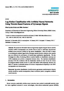
Figure 1 | The linear transform model of fMRI responses. Top row: hypothetical plots of Figureneuronal 1.9: The activity hemodynamic Left column shows a ’canonical’ HRF in reaverage over time.response. Bottom row: corresponding functional magnetic resonance imaging (fMRI)sponse responses. Left: hypothetical haemodynamic impulse response function (HIRF) to a brief burst of neural activity, showing the initial dip, the demeasured as the response to athe briefundershoot. pulse of neuronal Right: the fMRI layed peak and Rightactivity. column shows howresponse the HRF when is ex-the average neuronal activity alternates (at specific times) between three different states (high, pected sum for an extended of peaks in neural Figurethe medium and low), withtobrief transients each time series it switches from one state toactivity. another. Given taken from Heeger and Ress measured time course of neuronal activity, it is(2002). possible to compute (using convolution) the time course of the fMRI response. Most fMRI studies go the other way, to infer the underlying neuronal activity from the fMRI response. In the example shown, it is possible to estimate (using linear following neural increase inneuronal BOLD activity signaliniseach in fact found. regression, given activity, the HIRF) a theparadoxical relative amplitudes of the of the three The states, along the amplitude of the transients. reason for thiswith is that even though the neural activity leads to an initial increase in

oxygen consumption and a decrease in blood oxygen levels, this is followed by an increase in cerebral blood flow (CBF) and aofsubsequent of oxygenated blood because the intrinsicoversupply inhomogeneity in the magnetic

withininlarger vessels. canRess be modito that area of cortex, causing anfield increase BOLD signalThe (seeacquisition Heeger and (2002)

fied to de-emphasize theofBOLD signals from larger for a review). The BOLD signal is based on the interplay oxygen consumption, CBF

vessels, by suppressing signals that are associated with higher flow velocities . Other fMRI techniques have leading to an increase in fMRI studies at higher that field-strengths. been developed separately measure different components of the haemodynamic response: perfusionbased fMRI measures blood flow19,20, compounds can be The Hemodynamic Response injected into the blood stream to allow the measurement of blood volume21, and diffusion-based fMRI Due to the indirect nature of thetechniques signal generation, themeasure changechanges in BOLD repromise to insignal neuralinand 22 sponse to neural activity has a distinctive timecourse, known as excitation the Haemodynamic glial cell swelling that occur with . So far, there has been only a modest amount of work towards Response Function (HRF) as shown in Figure 1.9. The HRF has 3 distinct features, requantifying the relationships between theseactivity. different lating to the distinct aspects of the blood oxygenation in response to neural In fMRI techniques (for example, see REFS 20,23,24). the first second or so after a burst of neural activity there is a drop in signal, although it Second, the relationship between fMRI and neuronal can often be fairly subtle and it not alwaysdepends observable. This is believed to stimulation relate to the responses on the behavioural and and onoxygen the fMRI data-analysisrelated methods. In the initial increase in deoxygenated protocols, blood following consumption to neural days of fMRI waspeaking some concern that the signal activity. Subsequently there is a early larger increase inthere signal, ~6 seconds after the was derived entirely from large draining veins, and consequently that it would provide misleading information about the 25 spatial localization of neuronal activity. For example, presenting visual stimuli at two nearby locations in the visual field evokes neuronal activity at two nearby locations in retinotopic visual areas such as V1. If the fMRI signal were evident only in the large vessel(s), which and blood volume. BOLD contrast increases with field-strength (Yacoub et al., 2001b), 15,18

folded grey vein, one th corresponds de-emphasi in those ves experiment. by restricting sible to disti 1.5 mm in th considerabl reported in 1 discussed b might be cru of functiona There are su the experim affect the fid fore importa measure the the underlyi Third, th responses d measured an taneous acti within a reg a period of t the neuron fMRI signa neuronal ac the neurons of neurons; ronal popul rent source synaptic act electrical act different m they each re are just begi

Temporal s

In a typical images are c systematica evoke a larg genation in intensity in ±5%, but ty mean intens Accordin be possible presentatio stimuli (FIG.

C HAPTER 1: I NTRODUCTION neural activity, due to the subsequent increase in CBF and oversupply of oxygenated blood. It has been suggested that the initial dip may be more tightly correlated in space with neural activity than the influx of oxygenated blood, but generally the increase in signal is easier to measure. Following the peak in signal there is a decrease back towards baseline, an undershoot where the response is actually negative, and then a final return to baseline. This undershoot has been related to a number of physical properties both in terms of blood flow/volume (Buxton et al., 2005) and metabolic effects (van Zijl et al., 2012). An assumption that the HRF is proportional to the underlying neural activity allows the BOLD timecourse in response to stimuli to be modelled. This assumption is known as the linear transform model (Boynton et al., 1996), which assumes that the same HRF is evoked by a stimulus independently of how close in time it is presented to another stimulus, and that the HRF of stimuli presented close in time will sum together (superposition). Evidence for a ’rough’ linearity has been shown (Boynton et al., 1996), although a stimulus presented very soon after another (during a ’refractory’ period) will show a reduced response. This particular non-linearity can be exploited in experimental techniques such as fMRI adaptation. In general though, the BOLD signal in response to a sustained or repeated stimulus presentation is modelled by convolving a model HRF (the BOLD response to a brief stimulus) with the stimulus pattern. The amount of variance in the actual timeseries explained by this modelled timeseries can then be assessed. Full details of the process used to model the BOLD timeseries are given in Chapter 2.

Limitations and Improvements of BOLD fMRI Although the development of fMRI has allowed the non-invasive study of neural activity, there are a number of potential limitations to this method, stemming from the fact that the BOLD signal is a signal of hemodynamic origin with an indirect link to underlying neural activity. Some of these issues can be mitigated or avoided by specialized techniques or improvements in scanner technology. Others are inherent to the technique itself and cannot be avoided. A major consideration when using fMRI to study neural activity is the indirect nature of the BOLD signal. The exact link between neural activity and changes in BOLD signal is not fully understood, especially whether the coupling between the two is loose or tight. Combined recordings of neural activity , both in terms of neuron spiking and local field potentials (LFP), and BOLD in monkeys show that BOLD signal is more closely correlated with LFP than the spiking activity. LFPs are related both to post26

C HAPTER 1: I NTRODUCTION neuron synaptic activity and intra-neuronal processing, reflecting both the input to a neuron and its internal activity. This means that both excitation and inhibition of the cell can be reflected in the LFP, whereas an increase in spiking can only reflect excitation (Logothetis, 2008). Therefore drawing conclusion about neural activity can be non-straightforward based on an increase or decrease in the BOLD signal. Because of the hemodynamic nature of the BOLD signal, the spatial resolution of the BOLD signal may also be inherently limited. The BOLD signal in response to neural activity in a given area will reflect the contribution both from capillary beds that are tightly localized to the activity in question, and draining veins that may be spatially distant from the cortical area in question (Frahm et al., 1994). Two possible methods of increasing the spatial specificity of the BOLD signal exist: increasing the magnetic field strength and using spin-echo rather than gradient-echo imaging. Increasing the magnetic field emphasises the signal coming from spins in the tissue affected by the field inhomogeneities caused by de-oxygenated blood (the extravascular signal) over the signal from spins within the blood vessels themselves (the intravascular signal). This suppression of the intravascular (IV) signal is due to the shortening of T2 ⇤ for venous blood compared to tissue at higher fields (Yacoub

et al., 2001b), leading to the IV component of the signal decaying away more rapidly than the extravascular (EV) component. Thus the IV signal from large draining veins is suppressed at higher field strengths, increasing spatial specificity. However, for some imaging techniques such as GE imaging, the EV component of the signal can arise from both large and small vessels, which can reduce the spatial specificity of the signal. Using SE rather than GE imaging can suppress the EV signal from larger veins, leaving only the signal from the smaller vessels, although the sensitivity to the BOLD signal is reduced. Combing high-field imaging with SE image acquisition is thought to provide the most spatially specific signal (Yacoub et al., 2003), although at the cost of signal amplitude that precludes the use of SE imaging in most instances. It has also been suggested that the initial dip is more closely related to neural activity, representing the initial increase in de-oxygenated blood due to oxygen extraction in the capillaries after neural activity, whereas the subsequent peak represents an overcompensatory increase in oxygenated blood that is less spatially restricted (Menon et al., 1995). However, capturing the initial dip can be problematic, due to both its transient nature and due to the fact that it has a very small amplitude at lower fields, consistent with the suggestion it arises from effects in smaller blood vessels. This presents the possibility that it may be more apparent at higher field strengths (Yacoub et al., 2001a).

27

C HAPTER 1: I NTRODUCTION At higher field-strengths, both image SNR and BOLD signal magnitude are increased. Furthermore, an increase in field-strength can also allow an increase in resolution, which can allow an increase in BOLD contrast due to the reduction in partial voluming effects, where voxels contain a mixture of grey matter, white matter and CSF. Small voxels can also increase the functional contrast of the signal by isolating tissue with a uniform selectivity. However, in both cases there is a trade-off between voxel-size and SNR, which can set a minimum threshold for voxel size.

28


1.3

Experimental techniques

Over the years, a number of different analysis techniques have been developed for fMRI datasets. These include examining the change in amplitude between two blocks of task or stimuli or evaluating the change in the amplitude or shape of the HRF between trials of a given task or stimulus. One key similarity between these various techniques is that they either treat the timeseries from each voxel as separate from those around it during analysis, or alternatively average the timeseries from a number of voxels together prior to analysis. This approach to fMRI analysis can be described as univariate because only one variable, the timeseries from the voxels or ROI, is considered in the analysis at a time. Univariate analyses either yield statistical maps of activity across the brain, or a single value per ROI. One potential limitation of this approach for measuring neural activity is that the signal measured from a given voxel/ROI can include contributions from a number of cells with a range of different selectivities, which can make distinguishing between responses to certain stimuli (for example those for different orientations or directions of motion) problematic.

1.3.1

Adaptation

To investigate the functional properties of sub-voxel neural populations, without requiring very-fine spatial resolution images, a number of alternative methods have been developed. The first is adaptation, which has a long history of use in psychophysical and neurophysiological experiments. Exposure to a visual stimulus will affect the neural responses to, and the perception of, subsequently viewed visual stimuli. The nature of these changes can provide us with evidence about the neural mechanisms involved in visual perception. Perceptual adaptation exists in many domains, and motion stimuli provided one of the first examples of perceptual adaptation effects: extended viewing of a moving stimulus causes subsequently viewed stationary or ambiguous stimuli to be perceived as moving in the opposite direction (the motion after-effect) (MAE) (Thompson, 1880). Similarly, the apparent contrast of a grating displayed after prolonged exposure to a grating with similar properties will be reduced, and the reduction in apparent contrast depends on the similarity between the adapter and the probe (Blakemore and Campbell, 1969). Furthermore, the perceived orientation of a probe grating can be affected by extended exposure to another oriented grating. Adaptation effects for the detection and discrimination of direction of motion have also been found, with the strength of the effect depending on the similarity between adapter and probe (Hol and Treue, 2001). 29


Figure 1.10: Pre (Black) and post-adaptation (Grey) tuning curves for three exemplar neurons under three models of adaptation. The adapting stimulus in each case is the central stimulus. A) ’Fatigue’ model: responses are reduced after adaptation in proportion to initial response to adapting stimulus, with no change in tuning width. B) ’Sharpening’ Model: adaptation narrows the tuning curves around the adapting stimulus. C) ’Facilitation’ model: no predictions are made for changes in the tuning curves. Figure taken from Grill-Spector et al. (2006).

More recently, adaptation to higher-level stimulus properties, such as the perceived gender of faces, has also been demonstrated (Webster et al., 2004). Perceptual after-effects and changes in the detection and discrimination of stimuli provide evidence of selective neural mechanisms in the human brain. Psychophysical results can provide us with evidence as to the neural coding underlying perception, providing some of the first evidence of orientation and direction-selective neurons in the human visual system. The neural consequence of adaptation are not fully understood at this point. One popular model of the neural effects of adaptation is the so-called ’fatigue model’ (Figure 1.10, A). In this model, neurons selective for the adapting stimulus reduce their firing rates after extended or repeated exposure to that stimulus. This leads to a general reduction in firing rates across the population of cells, with the greatest reduction seen in the cells that respond most strongly to the adapting stimulus. Such a change in selective properties would have many potential benefits, such as increasing sensitivity for novel stimuli or optimising the dynamic range of the selective neurons. Measuring the tuning curves of cells after adaptation has demonstrated the fatigue model is sufficient to explain adaptation affects for orientation and motion in V1 cells (Kohn and Movshon, 2004). A second model suggests that adaptation instead leads to a narrowing (’sharpening’) of the tuning curves for selective neurons, leading to fewer neurons responding to subsequent presentations of that stimulus (Figure 1.10, B). Under this model, neurons

30

C HAPTER 1: I NTRODUCTION optimally selective for the adapting stimulus would see the least reduction in activity, rather than the greatest levels. Evidence shows that this model of adaptation may explain the effects of adaptation seen in MT for motion, contrasting with the ’fatigue’ like effects seen in V1 (Kohn and Movshon, 2004). A third model posits that tuning is unaffected by adaptation, instead suggesting that the processing of stimuli is made quicker (’facilitation’) (Figure 1.10, C). Different models of adaptation may apply in different brain areas and under different task/stimulus conditions (see Grill-Spector et al. (2006) for a review). Selectivity along a particular stimulus dimension can also be demonstrated in fMRI using the methods of adaptation (Grill-Spector and Malach, 2001). These methods use extended exposure to a stimulus followed by testing with a probe stimulus that either matches or differs from the adapter along the dimension of interest. The BOLD response to an identical stimulus will be reduced in areas sensitive to that stimulus. By measuring the response to stimuli that differ from the adapting stimulus, and seeing whether this reduction in BOLD response is stimulus selective, then neural selectivity for the dimension in which the stimuli differ can be inferred. Measuring the effects of fMRI-adaptation could potentially allow subpopulations of neurons with different selectivities to be differentiated, despite them being co-localised in a single voxel, and hence offers one potential solution to the limitations of fMRI sampling resolution (Grill-Spector and Malach, 2001). How these stimulus-selective reductions in BOLD signal are related to the neural and perceptual effects of adaptation is not fully understood at this point, so care must be taken when interpreting fMRIadaptation results in terms of the underlying neural responses.

1.3.2

MVPA

An approach that has recently been introduced is to treat the timeseries from multiple voxels as a single multivariate dataset, and to take the activity of many voxels into account when performing an analysis. One such technique is multivariate/multi-voxel pattern analysis (MVPA), which uses the patterns of activity across a number of voxels to create ’classifiers’ that can decide which stimulus or cognitive state led to a novel activity pattern. MVPA methods are particularly exciting as they raise the possibility that signals arising from individual populations of neurons or columns can be accessed at standard fMRI resolutions (Boynton, 2005). Even in cases where signals at the univariate (single voxel) level do not allow stimuli to be differentiated, if the pattern of activity from a number of voxels is consid-

31


Figure 1.11: 2 Voxel example of how multivariate methods allow classification of stimuli. The left panel shows a situation where the stimuli classes can be identified on the basis of single voxels (univariate). The middle panel shows a situation where the two classes overlap, but a linear decision boundary can be calculated when the 2 voxels are considered simultaneously. The right panel shows where a nonlinear decision boundary is required. Figure taken from Haynes and Rees (2006)

ered multivariately, stimuli can often be differentiated with greater sensitivity. This is demonstrated in Figure 1.11. Each point in the plots represents a trial, with the colour representing a different trial type (in this case orientation stimuli). The left hand panel in Fig. 1.11 indicates a situation where the two stimuli can be differentiated based on the responses of either voxel taken in isolation. The middle and right panels indicate situations where the univariate responses overlap, so the response of either voxel in isolation cannot be used to distinguish between the stimuli. However, in both cases considering the response of both voxels simultaneously allows the two stimuli to be distinguished, by calculating a decision boundary. Any response on one side of this boundary is classified as one stimulus class, anything on the other side is classified as the other stimulus class. The middle panel shows the linear case, which in the 2-dimensional class yields a boundary line. Activity patterns resulting from a large number of voxels are often used, in which the responses of N voxels are considered in an N-dimensional space. In such an N-d space, the classes are separated linearly by a hyperplane. This method can also be expanded to distinguish more than two classes, in which case multiple hyperplanes are used for each two-way classification. A large number of linear classifiers exist (Duda et al., 2001), including linear support vector machines (SVM) (Schölkopf et al. (1999), see Kamitani and Tong (2005, 2006) for application), linear discriminant analysis

32

C HAPTER 1: I NTRODUCTION (LDA) (Haynes and Rees, 2005a, 2006), and Gaussian Naive Bayes classifiers (Brouwer and Heeger, 2009). All of these different methods work by computing a weighted sum of voxel activity to calculate a linear decision boundary to decide whether an observed data-point belongs to a particular category. The right panel in Figure 1.11 represents a non-linear classification, which results in a curved decision boundary. Whilst non-linear classifiers can be more sensitive to the differences between stimuli than linear ones they are sensitive to over-fitting, and may indicate selectivity in areas where none exists. For this reason, linear classifiers are generally used in MVPA experiments (Tong and Pratte, 2012). The accuracy of the classifier is tested by cross-validation: training on one set of data from a subject, and testing on a separate set from that subject. Often the testing set will be data from a single run, and the training data will be data from the remaining runs, with each run being tested in turn. This procedure avoids training and testing a classifier on the same data. The classification accuracy will generally depend on the separability of the responses to the stimuli (the distance between the groups of points in N-dimensional space), the number of datasets available for training, and the number of voxels used to generate the patterns of analysis. In general, the more voxels are used the more accurate the classifier can be, although if uninformative voxels are added to the patterns they may simply add noise and reduce classifier accuracy (Yamashita et al., 2008). MVPA methods have been used to decode a wide range of stimulus properties, including orientation (Haynes and Rees, 2005a; Kamitani and Tong, 2005; Swisher et al., 2010), direction of motion (Hong et al., 2011; Kamitani and Tong, 2006; Seymour et al., 2009), eye of origin (Haynes et al., 2005), colour (Brouwer and Heeger, 2009; Seymour et al., 2009), binocular disparity (Ban et al., 2012; Preston et al., 2008), object category (Cox and Savoy, 2003; Op de Beeck, 2010) as well as conjunction of features such as colour and motion (Seymour et al., 2009). In addition MVPA methods have been shown to be able to classify which of two overlayed stimuli were attended to (Kamitani and Tong, 2005, 2006), which of two stimuli were perceptually dominant during binocular rivalry (Haynes and Rees, 2005b), and the perception of ambiguous motion displays (Brouwer and van Ee, 2007; Serences and Boynton, 2007a). Results such as this suggest that an observer’s conscious perception can be decoded, and have therefore often been referred to as ’mind-reading’, and have sparked a wide range of discussion as to the potential of these kind of techniques, and the potential ethical implications (Tong and Pratte, 2012). Although the use of multivariate techniques has increased greatly in recent years, it should be noted that the exact mechanism by which multivariate methods make use 33

C HAPTER 1: I NTRODUCTION of neural information is not fully understood and it has been suggested that caution should be used when interpreting MVPA results (Bartels et al., 2008). One key area of debate is the scale of the signal exploited, specifically whether MVPA methods allow the measurement of sub-voxel level information. For stimuli such as orientation, where neurons are arranged into columns on the cortical surface smaller than the resolution available to typical fMRI techniques, it has been suggested that classification results may be driven by unequal sampling of columns selective for different orientations by the voxels (Boynton, 2005), or local variations in columnar organization (Kamitani and Tong, 2005, 2006). Alternatively, the results may reflect more global, coarse-scale biases (Freeman et al. (2011); Op de Beeck (2010), but see Kamitani and Sawahata (2010); Swisher et al. (2010)). Whilst columnar arrangement of feature selective neurons may allow successful classification, a successful classification result is not necessarily evidence of the presence of columns (Bartels et al., 2008), and high-resolution fMRI (Yacoub et al., 2001b, 2007; Zimmermann et al., 2011) or optical imaging are necessary to provide further proof of such organization.

34

Chapter 2

General Methods This chapter summarizes the general shared methods that were used for each experiment in this thesis. This includes the methods to segment and flatten the cortical surfaces, the methods to identify the retinotopic visual areas, the fMRI scanning parameters and the various analysis methods.

2.1

Cortical Segmentation and Flattening

Although the spatial resolution of the EPI images conventionally obtained from fMRI is high in terms of localisation, it is generally not sufficient for BOLD activity to be related to the underlying neural anatomy (although recent high-resolution studies at 7T have showed sufficient resolution to allow this). It is generally the case that a highresolution anatomical image is obtained separately, onto which the functional data is overlayed. Often these images are T1-weighted due the good contrast between white and grey matter. However the cortical surface is folded and convoluted, so interpreting spatial locations on these 3D images can be difficult. A common method for dealing with this issue is to identify and extract the surface between the grey and white matter, inflate and flatten it, and display the functional data on this flattened representation of cortex. This method allows the spatial locations of functional data to be more easily visualized, and is particularly useful for the visualisation and analysis of retinotopic maps. The surface-extraction method begins with a T1-weighted anatomical image, which is preprocessed and segmented, and ends with two cortical surfaces per hemisphere, one representing the white-matter (WM)/grey-matter (GM) boundary and the other to the grey-matter/cerebrospinal fluid (CSF) border. The WM/GM boundary can then 35

C HAPTER 2: G ENERAL M ETHODS

A

B

C

Figure 2.1: Processing stream for cortical surfaces. The white-matter/gray-matter boundary is identified from the T1 weighted anatomy (A), and then expanded to find the gray-matter/CSF boundary (B). The WM/GM boundary can also be inflated to smooth out the cortical sulci and allow easier visualization (C).

be inflated and flattened and used to display the data. The extraction and inflation process for our data was performed using Freesurfer (Dale et al., 1999) (see Figure 2.1 for a description of the process). The preprocessing begins with registering the T1 anatomy (Figure 2.2 A) into Talaraich space, which is used to generate starting estimates for the location of WM and key areas such as the corpus callosum. This is followed by normalising the image intensities in the T1 image present due to magnetic field inhomogeneities, which could lead to problems in identifying the borders between tissue types, using a non-parametric method (Sled et al., 1998). Non-brain tissues are then removed (for example, skull stripping) (Figure 2.2 B) using a surface deformation procedure (Segonne et al., 2004). Following this, voxels within the image are identified as being WM based on their intensity and Talairach location. The hemispheres are identified and seperated from each other

36

C HAPTER 2: G ENERAL M ETHODS A

B

Figure 2.2: Examples of the original T1 weighted 3D image (A) and the preprocessed T1 weighted image with the calculated WM/GM (black) and GM/CSF (white) surfaces overlayed.

and the brain stem, with the hemisphere boundaries based on the likely location of the corpus callosum in Talairach space. An initial surface is then generated for each hemisphere by tessellation of the outside of the white matter mass for that hemisphere, followed by topology fixing. This initial surface is then deformed following intensity gradients to optimally place the gray/white and surface at the location where the greatest shift in intensity defines the transition to the other tissue class. Finally, this surface is then expanded to match the gray/CSF boundary in the same way (Dale et al., 1999) (Figure 2.2 B). Following the identification and extraction of these surfaces, the GM/WM boundary can be inflated (Fischl et al., 1999). Whilst displaying functional data on either the GM or WM surfaces extracted earlier allows greater appreciation of spatial localisation than display on the 3D anatomy image, the sulci can still hide a large amount of activation. By inflating the surface, the sulci are flattened out and activity can be more easily observed. FreeSurfer inflates the surface while attempting to minimize geometric distortions and maintain the relative geometric relationships in the surface topology. Often the analogy of inflating a crumpled paper bag is used, in that the surface is inflated without any expanding as the surface is not elastic (Pienaar et al., 2008). Once inflated, the curvature values calculated from the original folded surface are typically displayed on the inflated surface. Examples of in inflated surface with the curvature displayed are shown in Figure 2.3. The curvature has been binarized, so that dark areas indicate sulci and light areas indicate gyri. The calcarine sulcus has been indicated on the medial view.

37


Anterior

Posterior

Posterior

Anterior

Dorsal

Lateral

Ventral

Medial

Figure 2.3: Examples of inflated cortical surfaces from the lateral view and medial view. Dark areas indicate sulci, light areas indicate gyri. White dotted line indicates calcarine sulcus.

For the close inspection of data, for example examining retinotopic maps in visual cortex, a further stage of flattening a patch of the inflated cortex can be implemented. We utilised mrFlatMesh, part of custom written software (mrTools, VISTA), to obtain the flattened patches. medial A

B

dorsal

calcarine sulcus

ventral

Figure 2.4: A) The location of the flattened patch of cortex on the inflated cortical surface, centered around the occipital pole. B) The flattened patch of cortex, with the calcarine sulcus indicated by the white dotted line.

38


2.2

Retinotopic Mapping

The visual cortex is retinotopically organized, in that neurons with receptive fields covering adjacent points of the visual field are adjacent on the cortical surface. This organization, called retinotopy, allows the identification of early visual areas. The border between early visual areas (V1, V2, V3 etc.) is demarcated by reversals of the retinotopic map for polar angle. Retinotopic maps to identify these borders can be generated using techniques first described by Engel (Engel et al., 1997). The technique uses stimuli consisting of flashing "checkerboards" that change their position over time to create periodic patterns of activity in retinotopically-organized areas. Examples of these stimuli are shown in Figure 2.5 consisting of shapes formed from a checkerboard pattern, which reverses contrast rapidly to ensure the neurons at that retinotopic location are stimulated. Maps of eccentricity are measured using expanding and contracting rings of the pattern, whilst mapping for polar angle is measured using a rotating wedge stimulus. Although this specific stimulus set-up was originally used to retinotopically identify the visual areas, a wide range of different stimuli can produce equivalent maps (Dougherty et al., 2003; Dumoulin and Wandell, 2008). A

B

Figure 2.5: Stimuli used in the retinotopic mapping paradigm. A) Rotating wedge stimulus for polar angle mapping. B) Expanding/contracting ring stimulus for eccentricity mapping.

The mapping technique works by making use of the limited receptive fields of neurons in the visual areas. When the retinotopy stimuli pass over a point in the visual field, neurons with receptive fields centred on that area will be stimulated only when the stimulus is at that point. As the stimulus progresses, this leads to a travelling wave 39

fMRI response (% signal change)


10 0 −10

0

24

48

72

96

120

144

168

192

216

240

Time (sec)

Magnitude

600 400 200 0 0

10

20

30

40 50 Fourier component number

Coherence 0

0.25

0.5

60

70

80

Phase 0.75

0

1

π

2π

Figure 2.6: Examples of the analysis of retinotopic mapping data. Top Row: Timeseries of a voxel in retinotopic visual cortex in response to the mapping stimulus, and the fitted sinusoid at the stimulus repetition frequency. Middle Row: Fourier decomposition of the timeseries, showing a peak at the stimulus repetition frequency (red circle) and the second harmonic (blue circle). Bottom Row: Coherence (left) and Phase (Right) from the correlation analysis displayed on the anatomy.

of neural activity as the stimulus enters and leaves each receptive field in turn. If the stimulus moves across the visual field at a constant speed, the responses will differ only in their phase. Retinotopic mapping methods that depend on the phase of the temporal modulation to define the receptive fields are often called ’phase-encoded’ (Engel et al., 1997). Figure 2.6 demonstrates how these methods works. The top row shows a timeseries from a voxel in retinotopic cortex in response to the polar angle mapping stimulus, along with the fitted sinusoid at the stimulus repetition frequency. The middle row shows a Fourier decomposition of the timeseries, with a peak at the stimulus repetition frequency, in this case 10 cycles/scan (red circle). There is a second peak at 20 cycles/scan (blue circle), which is a harmonic of the fundamental frequency. To judge the strength of the response to the mapping stimuli, we use the coherence value, which

40

C HAPTER 2: G ENERAL M ETHODS is the amplitude of the response at the stimulus frequency divided by the total energy over all frequencies. An example of the voxelwise coherence values in response to the polar angle mapping stimulus are shown in the left hand figure on the bottom row. Elevated coherence values are seen in visual cortex. The phase of the sinusoid at the stimulus repetition frequency that best fits a voxels timeseries defines which location in the visual field that voxel best responds to, and can be used to colour code each voxel (Figure 2.6, bottom row). Visual cortices in left and right visual hemisphere can be seen to have different colours because these areas respond to the contralateral visual field. In both the eccentricity and polar angle mapping conditions, we collected half the scans with the stimuli moving in one direction (e.g. clockwise for the polar angle stimuli, and expanding rings) and half the scans with the opposite direction (counter-clockwise for polar angle mapping, and contracting rings). By combining across these different directions, we could estimate the phase of the response for each voxel independent of any lag in the BOLD signal caused by hemodynamic delay (Larsson and Heeger, 2006).

41


Eccentricity A

B

C

Figure 2.7: Example eccentricity map displayed on a flattened cortical patch for a single subject (A), and on the inflated surface (B). The parts of visual field corresponding to each phase value are shown in panel C.

An example of the eccentricity maps generated by the expanding and contracting ring stimuli is shown in Figure 2.7 on both a flattened patch of cortex (A) and the inflated surface (B). The colour at each cortical location indicates the point in space that area best responds to (C). The fovea is represented in posterior locations, centered at the occipital pole. In more anterior areas, the representation shifts towards the periphery.

42


Polar Angle

B

A

C

UVM

HM

LVM Figure 2.8: Example polar angle map displayed on a flattened cortical patch for a single subject (A), and on the inflated surface (B). The parts of contralateral visual field, from the Upper Visual Meridian (UVM) to the Horizontal Meridian (HM) and Lower Visual Meridian (LVM), corresponding to each phase value are shown in panel C.

The polar angle map generated by the rotating wedge stimuli is shown in Figure 2.8 on a flattened patch (A) and the inflated surface (B). The colour in each area corresponds to the visual angle in the contralateral visual field encoded at each position. Note that the representation of the contralateral visual field is inverted in V1. The horizontal meridian (HM) is represented at the centre of the calcarine sulcus. Moving dorsally towards the upper bank of the calcarine, the representation shift towards the lower vertical meridian (LVM), and then back towards the HM. Moving ventrally towards the lower bank of the calcarine, the representation shifts towards the upper vertical meridian (UVM), and back again. The reversals in direction of the phase mapping mark the borders between the visual areas.

43


A

B V7 V3ab V7

LO2 LO1

V3d V2d

V3ab LO2 LO1

V3d V2d

V1 V2v hV4 V3v

V1

UVM

V1 V2v V3v hV4

HM

LVM Figure 2.9: Polar angle map plus identified visual areas overlayed on a flattened patch (A) and the inflated surface. Reversals in the polar angle phase map were used to identify the borders between visual areas.

2.2.1

Identifying visual areas

The eccentricity and polar angle maps can be used to identify the borders between the early visual areas (Figure 2.9). V1 contains a full representation of the contralateral visual hemifield, with the contralateral HM represented at the centre of the calcarine sulcus. Area V1 is bordered by two cortical regions that form the dorsal and ventral halves of area V2 (V2d and V2v). Each of these regions represent one quarter of the visual field, V2d representing the lower visual field and V2v representing the upper visual field. The border between V1 and V2 lies at the representations of the LVM and UVM, where the direction of phase progession reverses, and moves back towards the HM. This pattern of reversal continues, with adjacent visual areas having mirrored polar angle maps travelling dorsally and ventrally away from V1. For example the V2/V3 border is marked by a phase reversal at the representation of the HM. The dorsal and ventral V3 maps then progress back towards the LVM and UVM respectively. V1, V2 and V3 share a foveal representation that makes it difficult to differentiate the areas at the most foveal part of the map, known as the area of foveal confluence. The mirrored phase representation found in V1-V3 changes slightly beyond this point, as non-identical visual areas are found on the dorsal and ventral sides. Area V4 borders 44

C HAPTER 2: G ENERAL M ETHODS V3v at the UVM, and from here the angular map progresses the whole of the contralateral hemifield, rather than just a quarter-field up to the HM. The exact nature of the V4 angular map is a subject of debate, specifically whether the visual hemifield representation is split dorsally and ventrally, or whether a complete hemifield representation exists within ventral V4, with no dorsal portion of V4 in humans (Tootell and Hadjikhani, 2001). For the purposes of this thesis we adopted the definition of hV4 as a full contralateral hemifield representation beyond V3v (Larsson and Heeger, 2006). On the dorsal side, V3 borders with 2 visual areas at the LVM. The LVM representation bifurcates around halfway along the border of V3d. The border above this bifurcation marks the border between V3 and V3A. V3A contains a full map of the contralateral hemifield (Wandell et al., 2005) extending dorsally. V3A shares a polar angle map with another area, V3B, with the boundary between the two areas being marked by a shared foveal representation separate from the one at the foveal confluence. As this boundary is not always clear, V3A and V3B are often combined into a single region referred to as V3AB (Larsson and Heeger, 2006). V3AB shares its anterior/dorsal boundary with V7 at the UVM, with V7 also containing a full representation of the contralateral hemifield (Press et al., 2001). The retinotopic maps beyond V3 were initially poorly defined, but recent studies have shown eccentricity and polar angle maps extending up to and through V5/MT. The LVM representation below the bifurcation in the V3d border marks the boundary between V3d and an area known as LO1 (Amano et al., 2009; Larsson and Heeger, 2006). LO1 also contains a full representation of the contralateral visual field, and borders with LO2 at the UVM. Similarly, the anterior border of LO2 is at the LVM. This border is believed to be the posterior border of MT/V5, which has been shown to contain a map of the contralateral visual field (Huk et al., 2002; Kolster et al., 2010). Amano et al. (2009) showed evidence of a full hemifield representation bordering LO2 at LVM which they called TO1, and an additional map with a border at the UVM that they named TO2, identified as a possible candidate for area MST. In the retinotopy data for our subjects however, LO1, LO2 and the retinotopy in MT+ were not always easy to identify, so LO1 and LO2 were not studied, and MT+ was identified with a within session localizer scan. MT was identified independently for each scanning session, as a uniform area identified from the separate retinotopy session was not always possible. In some scanning sessions a motion retinotopy stimulus was used as a localizer (Huk et al., 2002). The setup for this stimulus was identical to the rotating wedge stimuli described above, but in this case the wedge shape was defined by moving versus static dots (Figure 2.10).

45


...

Figure 2.10: The motion defined retinotopy stimulus used as a within session MT+ localizer in some sessions. Other sessions used the same arrangements of dots, but alternated all dots in motion versus all dots stationary.

The wedge was defined in a 24.6 diameter circular aperture filled with white dots on a black background (dot density 5 dots per degree2 of visual angle, dotsize = 0.1 deg). At a given point in time, dots within a 90 wedge moved toward and away from fixation (dot speed 8 deg/sec), while the rest of the dots within the aperture remained stationary. The wedge advanced 15 every second, completing a full revolution each 24s, and completed 5 revolutions each scan (total, 2 minutes per scan). In several other sessions, an MT+ localizer was used (Huk et al., 2002). This contrasted moving versus static dots for the whole field. This stimulus is known to yield activity in MT, MST and sometimes cells in the LO areas (Kolster et al., 2010). The use of within session retinotopy scans allowed us to compare retinotopy data collected at different resolutions and field strengths. The initial retinotopy data were collected at 3T at a resolution of 3 mm isotropic, additional sessions at 7T with the motion retinotopy stimulus were collected at 1.5 mm isotropic, and for one subject we collected an additional session of motion retinotopy at 7T with a resolution of 0.8 x 0.8 x 0.85 mm3 . Figure 2.11 shows the retinotopic maps for polar angle collected for the same subject in each different session displayed on the cortical surface. The phase reversals indicating the borders between visual areas are easy to identify at 3 and 1.5 mm, and appear to match up well. The high resolution phase map is less clear than at coarser scales, but the reversals at the edges of the calcarine sulcus can be seen. In both of the 7T datasets, the polar angle map in MT+ is clearer than at 3T, with a full map of the contralateral visual field apparent. The phase reversal between hMT and hMST can possibly be identified, which is not apparent in the 3T dataset. This is an example of

46

C HAPTER 2: G ENERAL M ETHODS the potential benefits of high-resolution fMRI, although also highlighting the reduced SNR at very high resolutions.

3mm (3T)

1.5mm (7T)

0.8mm (7T)

Figure 2.11: Comparing retinotopic maps for polar angle collected in 3 different sessions: a 3 mm isotropic session at 3T, a 1.5 mm isotropic session collected at 7T, and a 0.8 x 0.8 x 0.85 mm3 session also collected at 7T. Phase values from voxels with a coherence > 0.5 are displayed on the inflated (left) and flattened (right) cortical surface.

47


2.3 2.3.1

fMRI Methods Participants

All volunteers took part in the studies with written consent. Procedures were approved by the Medical School Research Ethics Committee of the University of Nottingham.

2.3.2

Visual Stimuli

Stimuli were generated using MATLAB (MathWorks) and MGL (available at http://justingardner.net/mgl) on a Macintosh Intel computer. Stimuli were displayed via an Epson EMP-8300NL LCD Projector onto a back-projection screen close to the bore of the magnet. Subjects viewed the projected stimuli through a set of mirror-glasses (maximum eccentricity of 16.2 degrees of visual angle).

2.3.3

Functional Imaging

BOLD data were collected on a Phillips 7T scanner, using either a 3D Gradient Echo EPI pulse sequence (TE=25ms, TR=85ms, FA =22 deg dynamic scan time=2s), or a 2D Gradient Echo EPI Sequence (TE=25ms, TR=2000ms, FA=78 deg), both with a voxel size of 1.5 mm isotropic and 34 slices through the brain. Initial piloting was done at 1.25 mm isotropic 3D GE EPI, but it was decided that this size did not have a high enough signal to noise ratio (SNR) to accurately measure BOLD signal. This highlights an important consideration in high-field scanning: the temptation may be to aim for the highest possible resolution to a) increase the localisation of signal and b) cut down on partial volume effects by increasing the likelihood of voxels containing only one kind of tissue, and ideally resolve a single column of neurons with the same selectivity. However, smaller voxels lead to a reduced amount of signal, which leads to a reduced SNR for some experimental paradigms that are not designed to maximise it. After initial higher-resolution imaging failed to resolve the HDR in event-related pilots, the voxel size was therefore increased to 1.5 mm isotropic. Distortions caused by inhomogeneities of the main (B0) magnetic field are especially problematic at 7T, and without correction the resultant brain images would be unusable. Before the scanning session began proper, it was necessary to take a measure of the B0 magnetic field, and calculate shimming values to combat distortions in the field. Test EPI images with the calculated shim values were manually examined, and retaken with altered parameters if necessary. This process, whilst essential for collecting good

48


A

B rostral

caudal

C

D

right

EPI (distorted)

T2* Anatomy

EPI (undistorted)

l

Figure 2.12: Examples of the images collected in a typical scan. A) Example of a whole head MPRAGE image, with typical stack placement in orange. The stack was placed to encompass the calcarine sulcus and temporal and dorsal visual areas B) Example EPI image collected during an experiment. The dashed line shows where the distortions cause the collected image to differ from the ’actual’ image. C) T2* weighted anatomical inplane image. This image has the same contrast as the EPI images, but doesn’t have the distortions D) EPI image after nonlinear alignment with the T2* weighted anatomy. This has corrected some of the distortions in the image, which would allow the data from the EPI images to be displayed on the whole head anatomy or cortical surfaces.

quality data, can potentially add 10-15 minutes to the scan time, which can be problematic if a large amount of functional data has to be collected. Subjects in the scanner for a prohibitively long session may become restless, leading to increased subject motion and reduced attention for the functional experiments. As a first analysis step, functional scans were aligned with an inplane anatomy image collected at the end of the scanning session. Initial piloting used a T1-weighted image (MPRAGE, voxel size = 1 x 1 x 1.5 mm3 ). In later sessions a high-resolution (0.5 ⇥ 0.5

⇥ 1.5 mm) T2*-weighted anatomical volume was collected during each scan session.

These images had the same slice prescription and coverage as the functional data (TE = 11 ms, TR = 608 ms, FA = 32 ). These scans took approximately 2 min. The T2* anatomy was used for nonlinear registration between the distorted EPI images and (intrinsically

undistorted) anatomy for each subject, and to calculate the warp fields necessary to correct for distortions (Klein et al., 2009). We used the nonlinear registration as a final step for visualization to project statistical maps calculated in the classification analysis (in the space of the originally acquired data) to be displayed on the subjects’ flattened cortical surfaces (in the undistorted anatomical space). Using this correction step also allowed ROIs defined in (undistorted) anatomy-space to be used when analysing the (distorted) 7 T EPI (BOLD) data. 49


Translation Translation (voxels)

0.4

0

0.35 0.3 0.25

X Y Z

0.2 0.15 0.1 0.05 0 − 0.05

−0.1

Rotation

−3

x10

7

0

Rotation

6 5

XY XZ YZ

4 3 2 1 0

Rotation

0.5

Figure 2.13: Example motion parameters for a single run for a single subject, showing

Rotation

0.45 0.4

0.35 0.3

translation (Top Row) and rotation parameters (Bottom Row).

0.25 0.2

2.3.4

Attention Control Task

Time (TR)

During each scan, the subjects performed a demanding two-interval forced-choice contrast discrimination task at fixation to control for changes in attentional state, which are known to modulate fMRI responses (Huk et al., 2001). The attention-control task consisted of a two-interval contrast discrimination task at fixation, with the threshold determined by a staircase. The timing of the intervals and response was separate from the timings of the functional tasks.

2.3.5

Data Analysis

FMRI data were motion-corrected within and between scans for each session using standard motion correction algorithms (Nestares and Heeger, 2000). A rigid-body transform was applied to align each volume to a reference volume, using 6 parameters (3 displacement parameters and 3 rotation parameters). Motion correction parameters for a single run for a single subject are shown in Figure 2.13. Motion correction statistics for each subject in the initial motion classification study are shown in Table 2.1, the mean Euclidean displacement within a single run, and the maximum frame-to-frame Euclidean displacement across a scanning session. Motion parameters for each subject and each session were manually examined to ensure no large motion-shifts that could interfere with successful classification (e.g. shifts larger than the size of a voxel). Linear trend removal was applied to the to the time course at each voxel. The timeseries from the voxels were converted to units of percent signal change by subtracting and dividing by the temporal mean for each voxel across each scan. The scans were then concatenated into a single 4D image. For fast-event related paradigm experiments, additional temporal high-pass filtering was performed. For the block design classifi50


mean across run (mm): max frame to frame (mm):

ab 0.55214 0.51357

jb 0.92598 0.49137

jp 0.65225 0.21273

rs 0.54903 0.15915

sh 0.76045 0.44233

Table 2.1: Motion statistics for the initial classification experiment, showing mean displacement across run (Top Row), and max frame to frame displacement across the entire experiment (Bottom Row).

cation experiments, no temporal smoothing or filtering was performed, although individual scans were detrended. Regions of interest for early visual areas were drawn from the separate session of retinotopy at 3T (described above), to allow identification on the undistorted cortical surface. The ROIs were transformed into the (distorted) EPI space for each subject and scanning session using the nonlinear alignment between the EPI images and the T2* weighted anatomy.

Deconvolution Analysis/Event Related Experiments Because the potential shape of the hemodynamic response function for each voxel in response to a brief presentation of motion was not known, a deconvolution analysis was used to estimate the response of voxels in visual cortex (Gardner et al., 2005). This method calculates a voxelwise average response to each stimulus type, and assumes that any overlap in responses results in a linear combination (Boynton et al., 1996), an assumption that holds approximately under many circumstances. The BOLD time course is modelled by the following equation:

[S1 S2 ... Sn ][ H1 H2 ... Hn ] T + noise = [ BOLD ] T

(2.3.1)

where Si is the ith stimulus convolution matrix with dimensions M x N, where M is the length of BOLD timeseries in TRs, and N is the length of the HDR we wish to calculate in TRs. A deconvolution matrix is a Toeplitz matrix with a 1 in the first column for any TR in which that stimulus was present. For example, a stimulus convolution matrix to calculate a 5 TR HDR for a stimulus presented on the 1st and 7th TR would take the form:

51


0 B B B B B B B B B B B B B B B B B B B B B B B B @

1 0

0

0 1

0

0 0

1

0 0

0

0 0

0

0 0

0

1 0

0

0 1

0

0 0

1

0 0

0 ...

0 0

1

C 0 0 C C C 0 0 C C C 1 0 C C 0 1 C C C 0 0 C C C 0 0 C C C 0 0 C C 0 0 C C C 1 0 C A

Hi is the 1 x N unknown HDR to the ith stimulus, T is the transpose operation and any noise is assumed to have gaussian distribution with zero-mean. BOLD is a 1 x M array containing the demeaned BOLD timeseries for a given voxel. The Hi for each stimulus is then computed for each voxel that minimizes the squared error between each side of the equation. An estimated timecourse could then be calculated for each voxel by multiplying the stimulus convolution matrices (S) with the estimated HDRs (H), and the amount of variance in the original timeseries explained by the model could be computed using the equation: r2 = 1

variance(residual ) variance(original )

(2.3.2)

where the residual timeseries is the difference between the estimated and original timeseries. This generated a voxelwise map of r2 indicating areas of the brain whose activity was modulated by the stimulus. The statistical significance of a given r2 was calculated using a permutation procedure (Gardner et al., 2005). The deconvolution analysis was repeated with randomised stimulus onset times, so the the times were no longer timelocked to measured activity. The r2 calculated from the HDRs found using these randomised times were assumed to represent the null distribution of r2 expected by chance correlations of noise in the timeseries with the stimulus timings. Any r2 from the distribution of actual r2 greater than a given threshold calculated from the null distribution (i.e. the 95th percentile) were considered to be significant.

52


Multivariate Pattern Analysis Multivariate pattern analysis (MVPA) was used to classify the patterns of activity in each ROI according to motion direction. The input patterns were created by averaging the activity in each voxel across each of the stimulus blocks, leading to one value per direction per run for each voxel. Voxels from each ROI were chosen on the strength of their response to the within-session (but independent) localiser stimulus, by selecting the 500 voxels with the highest coherence values. Support Vector Machine We utilized the LIBSVM toolbox to classify the observed directions of motion (Chang and Lin, 2011). A ‘linear ensemble detector’ for direction of motion was used to calculate a weighted sum of the voxel intensities in the input patterns: this was done by optimizing the weights such that the detector for each direction maximized its output for its preferred direction, and reduced it for other directions. The calculation for a linear ensemble detector for direction qk is a linear function of voxel inputs x = ( x1 , x2 , ..., xd )

gq k ( x ) =

d

Â w i x i + w0

(2.3.3)

i =1

where wi is the weighting for each voxel i and w0 is the bias. To construct the required weighting function for each direction, linear discriminant functions were calculated for each pairwise combination of directions using linear support vector machines (SVM). These pairwise discriminant functions were a weighted sum of the voxel inputs in the patterns, satisfying gq k q l ( x ) > 0

(2.3.4)

gq k q l ( x ) < 0

(2.3.5)

g being greater than 0 if x is a pattern of fMRI response induced by direction qk , and less than 0 for direction ql . A linear SVM found the optimal weights and bias for each discriminant function based on the training data set. The pairwise functions for a given direction versus all other directions were added together to yield the linear detector function for that direction. gq k ( x ) =

Â

m6=k

gq k q m ( x )

(2.3.6)

This function becomes greater than zero when the input vector x (voxel pattern of fMRI response) is one induced by its preferred direction qk . The test patterns are assigned to a given direction label based on which detector function yielded the largest output.

53


Figure 2.14: Examples of the 3D ’spherical’ searchlights. Using a searchlight with small radius (left) increase the precision with which informative areas can be located, but runs the risk of including too few voxels for successful classification. Increasing the radius of the searchlight (centre and right) increases the number of voxels available for classification, but reduces the precision with which informative areas of the brain can be localized.

Cross Validation To test the accuracy of the classifier, we used ‘leave one run out’ cross validation. The classifier was trained using the data on all but one of the runs, and then its accuracy at classifying the patterns from the remaining run was assessed. This process was repeated for each run in turn. This process assures the statistical independence of the test and training data, as they are drawn from separate runs. Significance Testing To test whether the classification accuracy in each ROI analysis was significantly above chance, we performed a non-parametric permutation test. 1000 classification analyses (using leave one-run out cross validation) were performed with the labels in the training data indicating which patterns of activity related to which direction of motion shuffled. This produced a distribution of classification accuracies expected under the null hypothesis that these patterns did not relate to the perceived direction of motion. These null distributions were used to create significance values for the actual accuracies, and accuracies from the correctly labelled dataset were considered significant if they were higher than the 95th percentile of this null distribution (p 0.4 in the lateral part of the brain were considered to correspond to the left and right portions of MT+. The voxels used to calculate the HDR to the probe stimuli were selected on the basis of the r2 thresholding method described above. For the initial coherence curves experiment, a p of 0.05 was used as the threshold for voxel selection. For the ’unadapted’ scans, voxels from right and left MT+ were combined. For the adapted scans, left and right MT+ were examined separately.

3.1.2

Results & Discussion

Figure 3.3 shows the calculated hemodynamic response curves from voxels in MT+ for a single subject for scans where the subject viewed incoherent dots during the adaptation periods in between trials. The curves show the expected pattern with the 100%

61

C HAPTER 3: P ILOT E XPERIMENTS : D IRECTION S ELECTIVITY IN MT+

Area MT+ 6

coherence

5

0.25 0.5

4

0.75 1

Scaled HRF % Signal change

3

2

1

0

−1

−2

−3

0

5

10

15

20

Time (sec)

Figure 3.3: HDR curves in MT+ for different coherence levels for a single subject using a deconvolution analysis

coherence curve having a largest amplitude, and the 25% response being the lowest, indicating a preference for coherent motion in MT+ as in previous studies (Becker et al., 2008; Braddick et al., 2001; Rees et al., 2000). The intermediate coherences lie in beMT+ tweenArea the two curves, although the are not fully separable or ordered, with the 50%

and 75% curves overlapping. This may just be due to variability in the responses to coherence these stimuli, or 0.25 it may be that the balance between the signal caused by activity relat0.5

ing the preferred,0.75anti-preferred and other directions may not allow these signals to be 1

differentiated (Braddick et al., 2001). Figure 3.4 shows the mean HDRs from right (incoherent motion adapted) and left (bidirectional motion adapted) MT+ ROIs in 2 subjects during the adaptation condition. The pattern suggested by the curves from the single subject remains in the ’incoherent motion adapted’ ROI, with the amplitude for the 100% coherence curve larger than for those of lower coherences. The curve for 0% coherence is lower still, although a slight increase in BOLD signal remains. This may be due to the fact that whilst a 0% 10 Time (sec)

15

20

coherent stimulus should not lead to any response in the ’incoherent motion adapted’ ROI (as it matches exactly the adapting stimulus), it will lead to a response in the ’bidirectional motion adapted’ ROI, which may lead to a general increase in attention for all trials. As changes in attentional state are known to affect activity in MT+ (Huk et al., 2001), this is a possible explanation for this anomalous activity. Nevertheless, the activity does not match that for the higher coherence stimuli. The curves for the inter-

62


0% coherence adaptation

Bidirectional adaptation

4

4

coherence=0 3

3

2

2

1

1

0

0

−1

−1

−2

−2

coherence=0.25 coherence=0.5


coherence=0.75

−3

coherence=1

−3

0

5

10 Time (sec)

15

20

0

5

10 Time (sec)

15

20

Figure 3.4: HDR curves for different coherence levels using a deconvolution analysis from MT+ during the adaptation condition for the ’incoherent motion adapted’ and ’bidirectional motion adapted’ MT+ ROIS. Errorbars indicate

±1 SEM across subjects (n=2).

mediate coherences overlap, so no exact ordering of responses can be shown. For the ’bidirectional motion adapted’ ROI, the ordering appears to be altered, with responses for low coherence stimuli elevated compared to high-coherence stimuli. However, the large standard error bars make it difficult to draw firm conclusions about the ordering of the coherence curves. Figure 3.5 demonstrates the potential problems in measuring coherence response curves using fMRI, namely the choice of baseline in between trials. HDR curves for different coherences were measured during a session where a subject viewed stationary dots in between probe stimuli, rather than incoherently moving ones. The amplitude of the responses to coherent, incoherent and intermediate coherence stimuli are all very similar, with some suggestion of larger responses for lower coherence stimuli. Voxels in MT+ responded just as strongly to incoherent motion as they did to fully coherent motion, seeming to indicate no kind of selectivity. However, this highlights the issues in attempting to create ’coherence response curves’ related to ’contrast response curves’: motion selective cells will still respond to incoherent motion, just less than to coherent motion at their preferred direction. In addition, motion onset can induce a large transient response that can mask any truly selective signal. Therefore, it may be the case that responses to different levels of coherence must be measured in terms of response to a change in coherence (e.g. a chance from incoherent to coherent motion), not by the sudden appearance of motion in a stimulus. 63


Area MT+ (246 Voxels)

2.5 2

0% 33% 66% 100%

1.5


1 0.5 0 −0.5 −1 −1.5 −2 0

5

10

15

20

Time (sec)

Figure 3.5: HDR curves for different coherence levels using a deconvolution analysis from MT for a single subject using static dots as the adaptation stimulus.

FMRI voxels, even the relatively small ones used in these initial experiments, will sample a large number of motion sensitive neurons, with a range of preferred directions, speeds and other stimulus properties. Although increasing the coherence of a stimulus may increase the activity of cells selective for the coherent direction, cells selective for other directions will reduce their activity as the number of dots moving in their preferred direction decreases, and may even be suppressed by the cells selective for the coherent motion. Combined with the uncertainty about the ratio between a selective signal and a non-selective ’global’ component in the BOLD signal, it is not simply the case that an increase in motion coherence will lead to an increase in BOLD signal. For the study of selectivity with neural architecture arranged at a scale less than that of typical fMRI voxels, other techniques may be required.

3.2

Adaptation

Extended exposure to a perceptual stimulus can affect the perception of a subsequent stimulus in a way that can provide evidence regarding the neural underpinnings of the perception of those stimuli (Clifford, 2002). Similarly, the amplitude of the BOLD response to a probe stimulus after extended exposure to an adapting stimulus can tell us about the selectivities of the neurons underlying that BOLD response in a given 64

C HAPTER 3: P ILOT E XPERIMENTS : D IRECTION S ELECTIVITY IN MT+ voxel or area (Grill-Spector and Malach, 2001). Outside of perceptual effects, adaptation can also affect the detection and discrimination of subsequently viewed stimuli (Clifford, 2002). Direction and orientation studies have shown that adaptation to a stimulus will make detection of that stimulus more difficult, for example bidirectional adaptation along an axis of motion causes coherence thresholds along that axis of motion to be elevated, even in the absence of an MAE (Hol and Treue, 2001). Adaptation orthogonal to the test direction has no effect, with adaptation increasing as adapter and test become more similar, revealing a direction specific elevation of detection thresholds. For two-interval discrimination the pattern is reversed, with directions close to the adapted direction being easily discriminated, whilst if adapter and test directions differed by around 20 degrees, discrimination thresholds were elevated (Hol and Treue, 2001). Neural selectivity for orientation has been demonstrated in a number of fMRI adaptation studies (Fang et al., 2005; Larsson et al., 2006; Sapountzis et al., 2010). BOLD responses in primary visual cortex to oriented grating stimuli were measured after adaptation to matching, orthogonal and varyingly separated stimuli (Fang et al., 2005). The amount of adaptation was orientation selective, specifically inversely proportional to the angular separation between test and adapter. Psychophysical adaptation tests done alongside the experiment found a similar relationship for contrast detection thresholds after adaptation. It is worth noting that initial studies found fMRI adaptation for orientation only in extrastriate cortex, and not in V1 (Boynton and Finney, 2003). These first studies used a very brief adaptation period (~1s), and when later studies extended this adaptation period to match with psychophysical studies, they actually found more adaptation in primary visual cortex compared to extrastriate areas. Therefore failure to find an adaptation effect does not mean that neural selectivity does not exist in the area under examination, it may be that the stimuli chosen as the adapter may not reveal it. FMRI adaptation has been used to show that BOLD responses are reduced when motion stimuli follow an adapter with the same direction of motion compared with an opposite one (30 s initial adaptation, 4 s top-up adaptation) indicating some level of direction selectivity (Huk et al., 2001). An additional experiment utilising an alternative adaptation method compared BOLD signal during blocks of stimulus presentation where stimuli moved repeatedly in the same direction with blocks in which a variety of stimulus directions were shown (Huk et al., 2001). Given that psychophysical adaptation has also shown direction-tuned effects for motion stimuli, we decided to investigate neural selectivity for motion direction using fMRI adaptation in a manner similar to the orientation studies by examining whether the amount of adaptation changed

65

C HAPTER 3: P ILOT E XPERIMENTS : D IRECTION S ELECTIVITY IN MT+ with the angular separation between adapter and probe.

3.2.1

Methods

A ’long-term’ adaptation paradigm was used, with a long initial adaptation and a period of ’top-up’ adaptation in between trials, as this had yielded good results in the Hol and Treue (2001) psychophysical adaptation experiments for motion and in earlier fMRI adaptation studies. Data were collected from 2 subjects on the 7T scanner, with the same scan parameters and data pre-processing as the pilot coherence study. ROIs were again identified using the retinotopy stimulus used in the pilot experiment, and the same fixation task was used to control attention. The main part of the experiment was an event-related adaptation paradigm. Stimuli consisted of the same dot patches in the left and right visual fields as used in the coherence study. Before the scan began, there was a 30s adaptation period bidirectional motion stimuli (50% moving upwards and 50% moving downwards) on the side to be adapted, and static dots on the unadapted side. Bidirectional motion was used to match the earlier psychophysical studies, and to avoid inducing an MAE that could potentially introduce an attentional confound (Huk et al., 2001). The event related trials during the scan consisted of a period of ’top-up’ adaptation (7-13s) followed a 1s motion probe stimulus either matching the adapted direction, or differing by an angular separation of up to 90 degrees (orthogonal), oriented towards fixation. Based on the previous psychophysical and fMRI adaptation experiments, we expected complete recovery from adaptation when probe and adapter were orthogonal to each other, but as the angular separation between adapter and probe is reduced, the amount of shared neural population processing the stimuli should increase, and therefore the reduction in signal due to adaptation should increase.

3.2.2

Data Analysis

The same deconvolution analysis (Chapter 2) used for the coherence experiment was used to generate HDR curves for the different directions.

3.2.3

Results & Discussion

Preliminary results (Figure 3.6) showed some adaptation effects, but it was difficult to establish statistical significance (beyond the trends seen in the data). Although it does appear that the hemodynamic response amplitude for the test direction matching

66



Unadapted Side

Adapted Side

3

3

2

2

Probe 0 90

1

1

0

0

−1

0

5

10

15

20

Time (sec)

−1

0

5

10

15

20

Time (sec)

Figure 3.6: Hemodynamic response curves from area MT from the ’unadapted’ side (i.e. ipsilateral to the adaptation stimuli) and the ’adapted’ (contralateral) side, for the probe directions matching (black line) and orthogonal (grey line) to the adapter stimuli. Errorbars indicate ±1 SEM (n=2).

adaptation is reduced (dir=0, black curve), with little adaptation seen for the orthogonal direction (direction=0, grey curve), there is a lack of a within session unadapted baseline for comparison. Comparing the adapted hemodynamic response curves with those from the ’unadapted’ side shows that the hemodynamic response curves are not equal on the unadapted side, highlighting that we cannot assume in this case that the difference in response levels between the directions are a result of the adaptation. It may be that the fixation task was not fully controlling attention, and some directions modulate attention, or that the adaptation in either visual field was not as spatially specific as we had assumed. A number of previous studies have demonstrated adaptation effects for motion. Reduced BOLD amplitude was found in MT+ (as well as V1 and V2) when the direction of a drifting grating matched that of an adapting grating compared to a probe grating of the opposite direction (Huk et al., 2001). Contrasting the BOLD signal during blocks of mixed directions of motion and blocks of constant direction showed a reduction in BOLD amplitude during the constant directions block for both gratings and plaid stimuli (Huk and Heeger, 2002; Huk et al., 2001), with the strongest effects seen in MT+. A recent study that used RDK stimuli to probe motion adaptation also found directionspecific adaptation effects in a variety of areas (Lee and Lee, 2012). The adaptation experiment demonstrates some of the difficulties of studying neural selectivity with fMRI. Previous studies have found varying levels of adaptation based on the stimulus and experimental parameters selected (Fang et al., 2005), with the relationship between the adapter and probe stimuli seeming to be a key concern. Re67

C HAPTER 3: P ILOT E XPERIMENTS : D IRECTION S ELECTIVITY IN MT+ sponse curves recorded from individual cells (stimulus strength on the horizontal axis, strength of response on the vertical axis) show an s-shaped curve, with the firing rate saturating as the stimulus increases in strength (i.e. contrast or coherence). After adaptation, this curve is ’shifted’ along the horizontal axis, meaning that a stronger stimulus is required for the cell at the rate it did pre-adaptation. The point at which the adaptation effect will be felt most strongly is on sloped part of the curve, i.e. before the firing rate saturates, meaning that a probe stimulus should be selected that lies on this part of the curve. We elected to use a low coherence (33%) probe, mirroring the low-contrast probes used in orientation experiments (Larsson et al., 2006; Sapountzis et al., 2010), as this strength of stimulus should lie on the desired part of the curve, although the low coherence may have led to a sub-optimal BOLD response. We initially attempted to find the ideal probe coherence in the experiments described in Section 3.1, but were unable to find the ideal coherence from these results. Therefore we tried to use a motion equivalent to the contrast stimuli used in earlier fMRI adaptation experiments, which may not have been the optimal stimulus in this case. There are also concerns that the measured effects of fMRI adaptation may not measure neural adaptation as understood in electrophysiological experiments, and may in fact indicate selectivity where there is none by shifting adaptation effects ’downstream’ (Bartels et al., 2008). Areas without selectivity for a stimulus condition can appear to have it in fMRI adaptation studies due to ’inheriting’ it from earlier areas. For example, area V4 demonstrated selective adaptation to motion direction in some studies (Huk et al., 2001), even though this area is normally thought to insensitive to motion. One hypothesis for this result is that while neurons in V4 do not adapt to motion, neurons in V1 (which output to V4) do adapt, meaning that V4 may show a reduction in BOLD response even though there is no adaptation or selectivity in that area. The study by Lee and Lee (2012) highlighted this issue in their study of direction-selective adaptation by showing that the adaptation effects they found in MT and MST could potentially be largely explained by the adaptation effects seen in earlier areas, indicating that the adaptation effects seen in these higher areas may just have been inherited from lower areas, with the possibility of no (or little) additional adaptation in these areas. Evidence for V1 being the source of adaptation effects also comes from the fact that adaptation in MT neurons has been shown to be position specific within the cells RF, to an area within the RF of a V1 input to the cell (Kohn and Movshon, 2003). MT neurons have however been shown to alter their tuning for direction of motion in a fashion not seen in V1 cells, and whether these additional changes reflect additional processing in higher areas or can be explained by inherited effects remains to be seen (Kohn and Movshon, 2004).

68

C HAPTER 3: P ILOT E XPERIMENTS : D IRECTION S ELECTIVITY IN MT+ The indirect neurovascular coupling between neural activity and the BOLD signal creates additional issues when interpreting adaptation results. The extent to which BOLD activity and neural spiking are linked is unclear, and it has been argued that an increase may reflect inhibitory or excitatory synaptic activity, rather than action potentials (Logothetis et al., 2001). This may lead to areas receiving adapted input displaying selective fMRI adaptation effects rather than the truly selective areas (Bartels et al., 2008), going beyond the ’inheritance’ issues discussed above and leading to the apparent locus of neural adaptation being ’shifted’ downstream. Adaptation in an fMRI experiment may not be enough to conclusively demonstrate neural selectivity in specific brain areas, but if a consistent adaptation effect can be shown it demonstrates that some kind of selectivity must exist in some part of the visual system

3.3

General Discussion

Summaries of some of the pilot experiments we performed indicate some of the difficulties encountered when studying neural selectivity for motion using standard fMRI methods, even using smaller voxels at a higher field-strength. Although directionselective cells in macaque MT are known to increase their activity as motion coherence in their preferred directions increase, the change in BOLD response for a given voxel given a change in coherence may not not be straightforward (Becker et al., 2008; Rees et al., 2000; Smith et al., 2006). Incoherent motion contains a large number of motion signals that will weakly activate a large number of direction selective cells. Therefore, although increasing the coherence will cause the cells tuned to that direction to fire more strongly, the cells tuned to other directions will still fire in response to the incoherent motion noise (although cells tuned to the other direction will suppress their activity), and this summed activity may equal or outweigh the activity from the cells responding the coherent motion (Braddick et al., 2001). In addition, the motion sensitive complex in humans typically identified in MRI (MT+) is generally considered to be made up of a number of motion sensitive areas (hMT, hMST etc) whose cells may have different responses to coherent and incoherent motion (Becker et al., 2008). The mixture of selectivites within a given voxel also makes studying the tuning of cells using fMRI difficult using standard univariate techniques. A common method of dealing with this is the use of adaptation techniques originally used in psychophysical studies, where the BOLD response to a probe stimulus is measured after prolonged exposure to an adapting stimulus, with a recovery from adaptation indicating that a separate population of neurons responds to the probe stimulus. Such methods have

69

C HAPTER 3: P ILOT E XPERIMENTS : D IRECTION S ELECTIVITY IN MT+ been used previously to demonstrate tuning for orientation and direction of motion (Fang et al., 2005; Huk et al., 2001; Larsson and Heeger, 2006; Sapountzis et al., 2010). Although such methods are able to circumvent the resolution issues of fMRI, the exact choice of stimulus parameters can be a key issue (Fang et al., 2005; Larsson et al., 2006), which may require extensive piloting, and interpreting a positive adaptation result can be problematic when deciding which areas show selectivity (Bartels et al., 2008). An alternative, and potentially more powerful method of demonstrating selectivity is the use of multivariate classification techniques. These methods have successfully been used to demonstrate selectivity for orientation and direction of motion (Kamitani and Tong, 2005, 2006), and in the case of orientation have been shown to be successful at discriminating differences in orientation finer than those possible with adaptation techniques (Sapountzis et al., 2010). In the next chapter I will examine multivariate classification of motion-direction in early visual cortex and MT+.

70

Chapter 4

Classification of Motion Direction 4.1

Classification with High Field fMRI

Multivariate pattern analysis has been shown to be able to ’decode’ stimulus properties from patterns of BOLD activity in fMRI. For example, the perceived direction of motion for a cloud of drifting dots can be decoded from the patterns of activity in early visual cortex and in MT+ (Kamitani and Tong, 2006; Serences and Boynton, 2007b). This is despite the fact that the voxel sizes used, typically ~3 mm isotropic in standard fMRI experiments at 3T, are much larger than those required to individually sample the underlying neural architecture, as each voxel contains tens of thousands of neurons with a variety of different tuning properties. Voxels of this size are also too coarse to directly sample cortical columns, the smallest neural feature likely to be directly measurable using magnetic imaging methods, which are at scales of less than 1 mm in humans. This presents a question: how can a stimulus specific signal be present in the voxel sizes typically used in fMRI? The reason that a single voxel normally lacks selectivity lies in the way it samples the underlying neural activity. A common way of thinking about a voxel is as a ’compactkernel filter’ (Kriegeskorte et al., 2010), where a voxel samples the neuronal activity pattern by averaging together the signal within its boundaries. To include the effects of hemodynamic blurring, a more accurate model has the voxel sampling the neuronal pattern via a Gaussian kernel. The voxel grid in this case can be thought of as creating a downsampled/blurred image of the neuronal activity pattern on the cortical surface. At standard resolutions, information at the scale of cortical columns should be too fine to resolve given the voxel sizes. The individual voxels would be unlikely to all contain identical proportions of neurons/columns selective for different orientations (or

71

C HAPTER 4: C LASSIFICATION OF M OTION D IRECTION other stimulus features), which could lead to slight biases for different stimuli for each voxel (Boynton, 2005). Although weak at the level of single voxels, these biases could be detected at the multivariate level by a classifier algorithm. This explanation represents a form of aliasing of fine-grained neuronal information into the coarser scale voxel pattern. The possibility that standard resolution fMRI could be made sensitive to fine-grained patterns of columnar activity at scales that cannot be represented directly in the voxel patterns (this being information in the ’hyper-band’ frequencies of the neuronal activity pattern, which are those above the Nyquist limit of the voxel sampling (Kriegeskorte et al., 2010)) has been called ’fMRI-hyperacuity’ (Op de Beeck, 2010). Arguments against the hyperacuity hypothesis stem from the fact that blurring or downsampling of the voxel patterns prior to classification does not degrade performance of the classifiers. Op de Beeck (2010) blurred the voxel patterns in response to orientated gratings with a Gaussian kernel prior to classification, and found performance unaffected using kernels of up to 8 mm Full Width at Half Magnitude (FWHM). Gaussian blurring reduces the fine-detail in a pattern, acting as a low-pass spatial filter that emphasises information at coarser spatial scales, so successful classification after the reduction of fine-scale information was taken as indication that information at a coarser spatial scale must be used by the classifier. Smoothing simulated neuronal data sampled by a standard voxel grid, with information at either a fine (< 1 mm) or coarse (> 4 mm) scale showed unaffected performance in the latter case, but not the former, further indicating a role for a coarse signal in classification performance (Op de Beeck, 2010). Evidence for a coarse scale signal was also found by Gardner et al. (2006), who found above-chance classification for orientation even when their voxels had been downsampled to an inplane resolution of 1 cm. Kriegeskorte et al. (2010) modelled classification results for stimulated eye based on ODCs and found that classification results should decline rapidly as voxel was size was increased, and that a larger voxel should be far less informative than the equivalent set of smaller voxels even when noise cancellation was taken into account. Results such as these were taken as evidence that the signal used by classifiers must lie at a much coarser scale than the fine-grained patterns of columnar activity. Counter to these arguments, it has been suggested that Gaussian blurring and downsampling may not prove that only coarse-scale information is used. Kamitani and Sawahata (2010) argued that Gaussian blurring does not actually remove high-spatial frequency information in an image, but simply scales down both the signal and noise in the high-frequency bands of a pattern. If the kernel used to filter the image is known,

72

C HAPTER 4: C LASSIFICATION OF M OTION D IRECTION the process is invertible and the original image can be recovered, indicating the continued presence of detailed pattern information after smoothing. Therefore, they argued that the unaffected performance after Gaussian blurring did not indicate the use of solely coarse spatial scale information by the classifier. Although results from smoothing/downsampling do not completely preclude fMRI hyperacuity via aliasing by voxels, it is unlikely to be the source of classifier performance for a number of reasons. 1) Any aliased signal would be fairly low in amplitude, due to the local averaging/Gaussian blurring taking place within each voxel acting as a kind of ’anti-aliasing’ filter (Kriegeskorte et al., 2010), reducing the projection hyper-band into lower spatial-frequency bands. Although this low-pass filtering will not be complete, the aliased signal is expected to be very low in amplitude. 2) The effect of head-motion on such aliased signals (Kriegeskorte et al., 2010). Moving the voxel-grid by even a small amount will completely change the aliasing patterns of the hyper-band information, in a way that is not possible to correct via motion-correction algorithms. Given the successful classification results seen in fMRI studies, where some head-motion is unavoidable, and especially given the fact that classification can work between different scanning sessions (Kamitani and Tong, 2005, 2006), fMRI hyperacuity via aliasing seems unlikely. 3) Additionally, band limitations in phase- and frequency-encoding directions of MR imaging make aliasing of hyper-band information extremely unlikely (Swisher et al., 2010). Whilst the aliasing of ’hyper-band’ information into lower spatial frequency bands appears unlikely given a standard model of the voxel, columnar patterns are unlikely to have information solely at these spatial scales. Random variation in the spatial distribution of columns should lead to biases amongst different voxels, manifesting as components of the pattern at a range of different spatial-frequencies, including those directly measurable with fMRI (Kamitani and Tong, 2005). This information is not aliased hyper-band information, but rather reflects low band neuronal-pattern information. Direct study of orientation columns in the macaque has shown that weak, low spatial-frequency signals of this type exist (Obermayer and Blasdel, 1993). High-resolution fMRI of cat visual cortex, at resolutions high enough to resolve individual orientation columns, followed by ideal high and low pass filtering (which offers greater spatial frequency isolation than Gaussian filtering) and multivariate classification analysis, showed that whilst classification was highest at the scale of the cortical columns themselves, the orientation signal was spatially broadband, extending to the scale of millimetres (Swisher et al., 2010). Low-pass filtering that obscured the orientation columns themselves still showed significant biases within voxels, with perfor-

73

C HAPTER 4: C LASSIFICATION OF M OTION D IRECTION mance remaining well above chance with filter sizes up to ~1 cm. High-pass filtering showed performance equivalent to the original images when pattern information at scales of ~1.3 mm were included, matching the average spacing between the orientation columns, with no increase in performance after the addition of coarser scale information. A similar pattern of results was seen in high-resolution fMRI of human visual cortex, with low-pass and high-pass filtering followed by orientation classification showing a strong orientation signal at the scale of ~2-10 mm, consistent with a signal originating from variation in the spatial distribution of cortical columns (Swisher et al., 2010). Although this result was found using ideal volumetric filtering, which removes rather than attenuates unwanted spatial frequencies, when the same analysis was performed with a Gaussian filter similar results were found, although the drop-off in performance for low-pass filtering was less steep than for ideal-filtering. This contrasted with the findings of Op de Beeck (2010) who found no drop in performance up to 8 mm FWHM. One possible explanation could be that Op de Beeck (2010) used 3 mm isotropic voxels, whereas Swisher et al. (2010) used 1 mm isotropic voxels. Swisher et al. (2010) reanalyzed data collected by Kamitani and Tong (2006) with 3 mm isotropic voxels, and found significant reduction in classification accuracy after 8 mm smoothing, again in contrast to the findings of Op de Beeck (2010). Swisher et al. (2010) hypothesized that the difference in findings may be due to differing levels of head-motion, as they found a single subject with a large amount of head-movement showed no loss in performance after 8 mm of blurring. Misaki et al. (2012) showed that the effects of smoothing or ideal filtering could vary from subject to subject, with some of the effects being due to headmovements, but some variability existing beyond this that could not be accounted for by head-motion (Misaki et al., 2012). Information at even coarser spatial scales has also been suggested as a potential source of classification performance, based on the findings of above chance performance after blurring (Op de Beeck, 2010) or subsampling (Gardner et al., 2006) prior to classification. Some potential coarse-scale biases that could be used by a classifier are global biases for certain stimuli types, for example biases for cardinal (Furmanski and Engel, 2000) or radial orientations, the latter of which has been demonstrated electrophysiologically in animals (Leventhal, 1983), and in humans and primates using fMRI (Freeman et al., 2011; Sasaki et al., 2006). A weak but reliable bias amongst voxels for radial orientations could be used by multivariate methods to decode orientation, without the requirement of signals arising from local variations in columnar distribution. Initial studies of orientation classification ruled out a role for a radial bias for orientation

74

C HAPTER 4: C LASSIFICATION OF M OTION D IRECTION based on the finding that removing the radial component of the pattern before classification did not harm performance (Harrison and Tong, 2009; Kamitani and Tong, 2005). Swisher et al. (2010) found some evidence of a radial bias for orientation, albeit an extremely weak one seen only when the data had been low-pass filtered extensively, and they concluded that any radial bias provided little information for a classifier. Evidence that orientation decoding may rely on larger scale biases came from Freeman et al. (2011), who argued that an analysis based on spatial filtering assumes that signals arising from a radial bias would appear exclusively at low spatial frequencies and columnar signals at higher frequencies. They demonstrated that this reasoning may not hold by showing that decoding of information known to have coarse scale organization and expected to have no contributions from columnar irregularities, angular position in a retinotopic map, also showed a detriment in classification after low-pass filtering. Using the same high- and low-pass filtering methods as Swisher et al. (2010), they showed the same pattern of results for orientation and angular-position classification, with an drop in performance after low-pass filtering and classification well above chance after high-pass filtering. Therefore they concluded that responses organized into a coarse map would lead to signals at multiple spatial scales, so impaired performance after low-pass filtering could not rule out a coarse-scale map driving classification performance. They additionally found that averaging voxels together in a way that preserved a bias for radial orientations, by averaging voxels together based on the independently measured representation of polar angle, showed preserved classification performance (Freeman et al., 2011). When the equivalent level of averaging was performed randomly, classification performance was strongly reduced. Removing the radial bias via projection reduced classification accuracy, leading them to conclude that a radial bias organized at a very coarse scale was both necessary and sufficient for successful orientation classification. The necessity for a radial bias for classification has been questioned, given that orientation stimuli without radial biases can be successfully classified using MVPA (Clifford et al., published on-line 26 April 2011; Hong et al., 2011; Kamitani and Tong, 2006; Mannion et al., 2009). Clifford et al. (published on-line 26 April 2011) hypothesised that the stimuli used in Freeman et al. (2011), a rotating grating stimulus similar to the rotating wedge stimulus used in retinotopy, may have been particularly dependent on a coarse scale radial bias. Classifying ’block design’ stimuli’, rather than the ’event related’ style stimulus used by Freeman et al. (2011), may be more dependent on columnar information at a range of spatial frequencies. In addition to neural pattern information at various scales, it has been suggested that

75

C HAPTER 4: C LASSIFICATION OF M OTION D IRECTION the neural vasculature itself may have some selectivity, based on it how it samples the underlying cortical maps (Kamitani and Tong, 2005). If draining veins sample selective columns non-homogeneously for example, they will attain some selectivity that can be imaged directly by the voxels, and it may be the case that vasculature is in fact organized around a columnar arrangement in a way that amplifies weak selectivity signals (Gardner, 2010). Empirical evidence for a selective signal arising from draining veins came from a high-resolution classification study that also collected T2 ⇤ weighted

venograms (Gardner et al., 2006), demonstrating large draining veins with orientation specific responses that could support successful classification even in heavily downsampled images. A study of decoding which eye was stimulated from patterns of responses in V1 at high-resolution also showed a contribution to decoding from draining veins that sample ODCs in a biased fashion (Shmuel et al., 2010). Selective signals were also found in voxels completely corresponding to grey matter at both high and low resolutions, possibly due to local variations in pattern of ODCs, indicating that venous signals were not the exclusive source of classification performance (Shmuel et al., 2007). However these studies were performed at a high magnetic field strength (7T) compared to earlier classification studies. Imaging at 7T is known to reduce the intravascular signal from veins compared to tissue, so it may be the case that venous signals are more dominant at standard field strengths (Shmuel et al., 2010). It may also be the case that the vasculature allows selectivity even without an explicit biased sampling of neuronal selectivity. Under this model the fine structure of the vasculature supplying the BOLD signal to each voxel causes that voxel to act as a ’complex spatio-temporal’ filter of the underlying neural activity pattern, rather than as a ’compact-kernel’ filter (Kriegeskorte et al., 2010). The aliasing of neuronal patterns at different spatial scales into the different spatial frequency bands is expected to be more complex than expected by a simple averaging model, and as the aliasing is done by the vasculature rather than the voxels themselves, the aliased signal will be less sensitive to shifts of the voxel grid due to head movement. Supporting this hypothesis, Kamitani and Tong (2005, 2006) were able to show classification between scanning sessions for individual subjects, where the sampling of neurons/columns by the voxel grid is very unlikely to the same from session to session, due to the inability to exactly replicate the position of the voxel sampling grid with regards to the subject. The exact contribution from the neuronal pattern as sampled by the voxels, whether via local variations captured directly by voxels or a coarse scale map, and the signal sampled via the vasculature itself, whether due to biased sampling or a complex spatiotemporal filter, to classification performance is an ongoing area of debate (Kriegeskorte

76

C HAPTER 4: C LASSIFICATION OF M OTION D IRECTION et al., 2010). A study modelling classification accuracies of stimulated eye via ODCs based on a ’compact-kernel’ model of voxel sampling concluded that whilst hyperacuity could be ruled out, local variations in the pattern of ODCs that could be captured by the voxels were sufficient for above chance classification (Chaimow et al., 2011). However, the classification accuracies they found in the model were less than those typically found in classification experiments, leading them to conclude that coarsescale signals and some form of vascular contribution, be it biased sampling or complex spatio-temporal filter, must contribute the additional selective signal. Whilst neuronal pattern information, whether in the hyper-band or at spatial scales directly measurable by the voxels, and vascular selectivity are all ultimately related to neuronal activity, and therefore measures of neuronal selectivity, the exact localisation of the signal used by the classifier can be important if strong conclusions about the underlying neural signal are to be drawn. Therefore establishing the scale of the information used by classifiers is important if we wish to draw conclusions about the neural architecture in a given area. Previous analyses of motion selectivity have found that the perceived direction of motion of a drifting cloud of dots could be decoded from patterns of fMRI activity in both early visual cortex and MT+ in humans (Kamitani and Tong, 2006; Serences and Boynton, 2007b). Classification was well above chance for data from all areas, with no greater classification accuracy in MT+ compared to V1, despite this area’s assumed high proportion of direction selective neurons. Based on these previous reports, we attempted to replicate this result using higher-resolution fMRI at 7T, to see if we could draw any conclusions about the scale of the signal used in the classification of direction of motion. Moving to this higher field allowed the voxel size to be reduced from the 3 mm isotropic voxels used in the original study to 1.5 mm isotropic voxels, an eightfold reduction in volume. If successful classification is in fact based on the distribution of columns between voxels, then decreasing the size of the voxels should increase the amount of information available to the classifier by increasing the biases available present in each voxel (Kriegeskorte et al., 2010). However, if information is in fact carried by a signal at a coarser scale, then increasing the resolution may be likely to have little to no effect on performance (Gardner et al., 2006; Op de Beeck, 2010). Additionally, although the voxels in the current experiment are slightly larger than those used by Swisher et al. (2010) (1 mm3 versus 3.375 mm3 ), using smaller voxels than those used in standard fMRI experiments allows us to investigate contributions of variations in the spatial pattern at a scale smaller than these voxel sizes to classification.

77

C HAPTER 4: C LASSIFICATION OF M OTION D IRECTION

direction

coherence 1.0 dot speed: 8º/s annulus 2º – 12.5º

Figure 4.1: Examples of stimuli used in motion classification scans. All the dots in the field drifted in a common direction (white arrow), which changed every 16s. Note that the dot density and size are not to scale in this illustration. In the actual stimulus display, dot density was 5 dots per /deg2 and dot size was 0.1 deg

4.1.1

Methods

Subjects Five subjects experienced in fMRI experiments and with normal vision participated in this study with written consent. Procedures were conducted with approval from the University of Nottingham Medical School ethics committee.

Stimuli and Task Two experimental paradigms were used in each scan session: 1) A minimum of two scans of the motion retinotopy experiment detailed in Section 2.2, and 2) a block paradigm with motion in one of eight possible directions. The block-classification stimuli consisted of white dots in a circular aperture (diameter 24.6 of visual angle) (Figure 4.1). For these stimuli, all the dots drifted in the same direction at the same time for blocks of 16s (order randomized), following the paradigm of (Kamitani and Tong, 2006), with a block of fixation at the beginning and end of each scan (total, 2 minutes 40 seconds per scan). The dots had a lifetime of 200 ms. Subjects completed 16-20 of the classification runs per scan-session. To control for the effects of changes in attentional state, subjects performed a contrast discrimination task at fixation (as detailed in Section 2.3.4).

78

C HAPTER 4: C LASSIFICATION OF M OTION D IRECTION

Right

Left V3ab

V3ab

V3d V2d

AB

V3d V2d

V1

V1

0

MT+

MT+ V2v V3v

V2v hV4 V3v

0.25 hV4 0.5

Accuracy

V3ab V3ab

JP

V3d V2d V1

V3d V2d

0.75

V1

1 MT+

MT+

V2v hV4

V3v

V2v V3v

hV4

Figure 4.2: Classification accuracy maps derived from a searchlight classification analysis using a spherical searchlight with a radius of 3 voxels. Voxels are thresholded on the basis of a binomial test (p

Studying neural selectivity for motion using high-field

Studying neural selectivity for motion using high-field

Suggest Documents

Visual Representation Model for Motion Direction Selectivity

Studying Circular Motion - KLiC

Motion Path Design for Specific Muscle Training Using Neural Network

Studying the neural bases of prism adaptation using ...

Color selectivity in motion aftereffect - Springer Link

Using Deep Learning for Compound Selectivity Prediction

Selectivity Estimation for Joins Using Systematic ...

Neural structures for visual motion tracking - SmartLab

Qualification Specification - Highfield Awarding Body for Compliance

Neural selectivity for communicative auditory signals in Phelan ... - Core

A MOTION PLANNING APPROACH TO STUDYING MOLECULAR ...

On human motion prediction using recurrent neural networks

Motion Correction in MRI using Deep Convolutional Neural Network

Robot Motion Planning Using Neural Networks: A ... - Semantic Scholar

Leg Motion Classification with Artificial Neural Networks Using ... - MDPI

Muga Potash Mine - Highfield Resources

Motion Estimation Using a General Purpose Neural Network Simulator

Muga Potash Mine - Highfield Resources

motion planning of an autonomous mobile robot using artificial neural

Highfield Campus - University of Southampton

Animal models for studying neural crest development - Semantic Scholar

Non-mammalian models for studying neural development and function

An Artificial Body for Studying the Computational Properties of Neural ...

Studying Turbulence Using Numerical Simulation