Hindawi Publishing Corporation Journal of Robotics Volume 2013, Article ID 810909, 10 pages http://dx.doi.org/10.1155/2013/810909
Research Article Motion Path Design for Specific Muscle Training Using Neural Network Kenta Itokazu, Takanori Miyoshi, and Kazuhiko Terashima Toyohashi University of Technology, Hibarigaoka 1-1, Tempaku-cho, Toyohashi, Aichi 441-8580, Japan Correspondence should be addressed to Kazuhiko Terashima;
[email protected] Received 19 July 2013; Accepted 27 September 2013 Academic Editor: Shigeyuki Suzuki Copyright © 2013 Kenta Itokazu et al. This is an open access article distributed under the Creative Commons Attribution License, which permits unrestricted use, distribution, and reproduction in any medium, provided the original work is properly cited. Specific muscle training is expected to be used for efficient rehabilitation and care prevention. In this paper, we propose algorithms for designing a motion path capable of strengthening specific muscles. By using the proposed algorithms, it is possible to design a motion path maximizing the activity of an agonist muscle and minimizing that of other muscles. For training, the load is applied by using a 2-link arm. EMG signal is measured during a training experiment, and the degree of muscular revitalization is evaluated by the amplitude of EMG signal. Finally, the effectiveness of the proposed approach is demonstrated through experiments.
1. Introduction In recent years, in the context of the emergence of population ageing as a social issue in developed countries, the importance of regaining muscle strength for care prevention has become increasingly apparent. Prolonged immobility induces muscle weakness, which affects activities of daily living (ADLs) directly. Much research is being done on rehabilitation robotics that is pertinent to strength training. Lum et al. indicated that, compared with conventional therapy techniques, robotassisted training is more efficient for improving muscle strength and path-following capability [1]. For lower limb rehabilitation, Akdo˘gan and Adli developed a therapeutic exercise robot that enables rehabilitation for spinal cord injury in diverse ways, including both isotonically and isometrically [2]. Such research aims to regain a muscle strength of an entire arm or leg. Therefore, the robots are unable to apply a load to specific muscles. However, the degree of muscle weakness differs according to each muscle. Thus, the application of a load to specific muscles that require strengthening is expected to lead to more efficient and safer training. In the authors’ previous research, a method of estimating muscle force or level of muscle activation was proposed [3].
Though the objective of the research was to strengthen a muscle by isometric exercise, an isotonic exercise is more effective for ADLs training. The purpose of the present work is to develop an algorithm for designing a motion path capable of strengthening specific muscles for isotonic exercise. The method proposed in previous research does not consider the coordinated motion of an antagonistic muscle. However, when doing an exercise, an antagonistic muscle works to increase the stiffness of each joint, such as a shoulder or an elbow. A method of estimating muscle activity should consider the coordinated motion. In this paper, a neural network is used since it is suited to estimation of nonlinear data such as muscle activity. First, the neural network is trained by a backpropagation algorithm. A training data differs according to each subject person. The neural network is able to estimate the level of muscle activation. Secondly, we design the optimal motion path by using a multiobjective optimization method for the obtained neural network. The objective of optimization is to maximize the activity of an agonist muscle and minimize the activity of other muscles. The motion paths obtained by an optimization method for the learned neural network model are evaluated through experiments, and the validity of the proposed approach is then demonstrated.
2
Journal of Robotics y
6 axis force sensor
f, v
D x
m 𝜃2 DC motor Emergency stop switch
D
J2
Rotary encoder
𝜃1
Figure 1: 2-link arm.
J1
Figure 3: Virtual mass and viscosity.
Figure 2: Appearance of experiment.
2. System Description 2.1. System Structure. Figure 1 shows overall look of the 2-link arm that is used as a training device. There are DC motors and rotary encoders at each joint, and 6-axis force sensor at the end-point. An emergency stop switch is mounted. The device enables training of upper limbs by horizontal motion. Figure 2 shows appearance of an experiment. The EMG sensors are attached to the subject’s arm. 2.2. Control System. An end-point velocity of the device is controlled by force feedback. To apply a load to muscles, virtual mass and viscosity are set at the end-point (see Figure 3). A motion equation of the end-point is described by 𝑚 ⋅ a + 𝐷 ⋅ k = f,
(1)
where 𝑚 is virtual mass, 𝐷 is virtual viscosity coefficient, f = (𝑓𝑥 , 𝑓𝑦 )𝑇 is force measured by force sensor, and a = (𝑥,̈ 𝑦)̈ 𝑇 and k = (𝑥,̇ 𝑦)̇ 𝑇 are acceleration and velocity of the end-point, respectively. The control input for motors is given by k𝑖+1 = a ⋅ 𝑑𝑡 + k𝑖 ,
s = 𝐾Θ̇ 𝑖+1 ,
where 𝑑𝑡 is a sampling time set as 1 [msec], Θ̇ = (𝜃1̇ , 𝜃2̇ )𝑇 is angular velocity of each joint, and 𝑆1 , 𝐶1 , 𝑆12 , and 𝐶12 are sin 𝜃1 , cos 𝜃1 , sin(𝜃1 + 𝜃2 ), and cos(𝜃1 + 𝜃2 ), respectively. Furthermore, s = (𝑠1 , 𝑠2 )𝑇 is input signal, 𝐾 is conversion coefficient, and 𝑙1 and 𝑙2 are length of upper arm and lower arm that are set as 0.26 and 0.3 [m], respectively.
3. Neural Network 3.1. Outline. In this study, three-layer Artificial Neural Network (ANN) consisting of an input layer, a hidden layer, and an output layer is used, as shown in Figure 4. The inputs of ANN are joint torque (𝑇1 , 𝑇2 ) and joint angle (𝜃1 , 𝜃2 ), as shown in Figure 5. And, the outputs are level of muscle activation described as 𝛼̂1 , . . . , 𝛼̂5 .𝛼1 , . . . , 𝛼5 are measured values. The level of muscle activation 𝛼1 , . . . , 𝛼5 is defined as 𝛼𝑖 (𝑡) =
−1 Θ̇ 𝑖+1 = 𝐽𝑖+1 k𝑖+1 ,
𝑙𝑆 𝑙 𝑆 +𝑙 𝑆 J = [ 1 1 2 12 2 12 ] , 𝑙1 𝐶1 + 𝑙2 𝐶12 𝑙2 𝐶12
Figure 4: Neural network.
(2)
EMG𝑖 (𝑡) (𝑖 = 1 ∼ 5) , max EMG𝑖
(3)
where EMG𝑖 (𝑡) is electromyographic (EMG) signal that is measured during an experiment. max EMG𝑖 is maximum EMG signal for each muscle. During an experiment, EMG signals of muscles shown in Table 1 are measured.
Journal of Robotics
3
Table 1: Measured muscles.
0.13
𝑀1 𝑀2 𝑀3 𝑀4 𝑀5 y
0.12 0.11 0.1 RMSE
Name Pectoralis major Latissimus dorsi Brachioradialis Triceps brachii Lateral head Biceps brachii
0.08 0.07
F
0.06
𝜃
0.05
x
𝜃2
0.09
0.04
T2
2
4
6
8 10 Number of units
12
14
16
Figure 6: RMSE for various number of units in hidden layer. 𝜃1 0.25
T1
0.2 0.15
Figure 5: Upper limb model.
0.1
The number of hidden units is determined by comparing root-mean-square errors (RMSEs) of estimation results. RMSEs are calculated by RMSE = √
1 𝑁 2 𝛼 − 𝛼𝑖 ) . ∑(̂ 𝑁 𝑖=1 𝑖
=
𝑁=4
(1) (1) 𝑥𝑛 ∑ 𝑤𝑛,𝑗 𝑛=1
𝑦𝑗(1) = sigmoid (𝑆𝑗(1) + 𝑏𝑗(1) ) , 𝑁=10
0.2 0.25 0.25
0.2
0.15
0.1
0.05
0 0.05 x (m)
0.1
0.15
0.2
0.25
Figure 7: Motion path for exploratory experiment.
(5)
𝑛=1
𝛼𝑖 = sigmoid (𝑆𝑖(2) + 𝑏𝑖(2) ) , sigmoid (𝑧) =
0.1
motion on horizontal plane as shown in Figure 7. During the experiments, the motion paths, force, and position of the end-point are displayed on a monitor. The displayed force and end-point position are updated in a real time. And then, subjects follow the paths at a constant force (30 [N]). The ANN is trained by a backpropagation algorithm.
(𝑗 = 1 ∼ 10) ,
(2) (1) 𝑦𝑛 (𝑖 = 1 ∼ 5) , 𝑆𝑖(2) = ∑ 𝑤𝑛,𝑖
0 0.05
0.15
(4)
Figure 6 shows RMSEs of estimation results obtained using ANN that is trained by training data-sets as described in Section 3.2. Even where there are more than 10 units, RMSE is virtually unchanged. Therefore, we set the number as 10. The outputs of ANN are calculated by 𝑆𝑗(1)
y (m)
0.05
1 , 1 + 𝑒−𝑧
4. Motion Path Design 4.1. Outline. To design motion paths, we proposed two algorithms (i) algorithm for designing a motion path that always has the same initial posture (Algorithm 1),
where 𝑥 is input (joint torque and angle), 𝛼 is output (level of muscle activation), 𝑤 is connection weight, and 𝑏 is bias.
(ii) algorithm for designing a motion path that passes through the most effective point (Algorithm 2).
3.2. Training of Neural Network. In order to determine connection weights and biases, training of ANN is required. The training data sets are obtained through exploratory experiments for each subject. The data is measured during linear
These algorithms use a multiobjective problem. When designing a path using Algorithm 1, the initial value of multiobjective problem is the same for each time. Therefore, the designed paths for each muscles (𝑀1 ∼ 𝑀5 ) have the same
4
Journal of Robotics
initial position. The motion path designed by Algorithm 1 does not necessarily pass through the most effective point that is capable of maximizing the activity of an agonist muscle and minimizing the activity of other muscles. By contrast, Algorithm 2 designs a motion path based on the most effective point.
Start
Determine direction of force by Eq (6)
4.2. Algorithm 1. The algorithm uses ANN and multiobjective optimization to design motion paths. Figure 8 shows a flowchart of the algorithm. First, define an initial posture as 𝜃1 = 𝜋/4 [rad] and 𝜃2 = 𝜋/2 [rad]. Next, solve an optimization problem as shown below to satisfy both: max 𝜃
min 𝜃
Pose computation by Eq (7)
𝛼𝑛 (𝜃) 2
𝛼 (𝜃) , 𝜎 (𝜃)
√ x2 + y2
Yes
>0.2
(6)
subject to 0 ≤ 𝜃 < 2𝜋, where 𝜃 is direction of force, 𝛼𝑛 is level of muscle activation for target muscle, and 𝛼 and 𝜎2 are average and variance of nontarget muscles. 𝛼𝑛 , 𝛼 and 𝜎2 are calculated by using ANN. The aim of this optimization problem is to maximize the activity of an agonist muscle and minimize the activity of other muscles. In order to solve the optimization problem, sequential quadratic programming method is used. The method is also used to solve (8) and (9). To calculate the velocity from end-point force, (1) is simplified by setting 𝑚 = 0. By solving the optimization problem, we obtain the optimal direction of force. Thirdly, calculate the position of the endpoint. The position is calculated by 𝐹 |𝐹| cos (𝜃) ], f = [ 𝑥] = [ 𝐹𝑦 |𝐹| sin (𝜃) 𝐹𝑥 [ 𝐷] 𝑉 ], k = [ 𝑥] = [ [ 𝑉𝑦 𝐹𝑦 ] [𝐷]
𝜃̇ Θ̇ = [ 1̇ ] = J−1 k, 𝜃2 𝜃 ̇ Θ = [ 1 ] = ∫ Θ𝑑𝑡, 𝜃2
(7)
𝑇 T = [ 1 ] = J𝑇 f, 𝑇2 𝑙𝑆 𝑙 𝑆 +𝑙 𝑆 J = [ 1 1 2 12 2 12 ] , 𝑙1 𝐶1 + 𝑙2 𝐶12 𝑙2 𝐶12 𝑥 −𝑙 𝐶 − 𝑙 𝐶 P = [ ] = [ 1 1 2 12 ] , 𝑙1 𝑆1 + 𝑙2 𝑆12 𝑦 where F is end-point force, |𝐹| is absolute value of end-point force that is set as 30 [N], V is end-point velocity, P is position of end-point, Θ̇ and Θ are angular velocity and angle of joint, and T is joint torque. And 𝑑𝑡 is sampling time that is set as
𝛼 < 0.5 Yes End
Figure 8: Flowchart of Algorithm 1.
1 [msec], 𝐷 is virtual viscosity coefficient that is set as 900 [Ns/m], and 𝑙1 and 𝑙2 are length of upper arm and lower arm that are set as 0.26 and 0.3 [m]. By repeating the procedure until the distance between end-point position and origin exceeds 0.2 [m] or level of muscle activation of target muscle is less than 0.5, a motion path is designed. Figure 10 shows an example of a designed motion path. 𝑃1 ∼ 𝑃5 express motion paths of strength training that target each muscle (e.g., 𝑃1 targets 𝑀1 ). In this algorithm, these paths have the same initial position. 𝑀1 ∼ 𝑀5 have different function of arm movement. The shown paths are designed to enhance muscle activation of target muscle. Therefore, direction of the paths depend on the function of each muscle. For example, 𝑃1 shows adduction movement of shoulder, because 𝑀1 has function of shoulder adduction. 4.3. Algorithm 2. In Algorithm 2, most effective point that is capable of maximizing the activity of an agonist muscle and minimizing the activity of other muscles is calculated before designing a motion path to use in (9) as an initial value. A posture to take the most effective point is given by max
𝛼𝑛 (𝜃, 𝜃1 , 𝜃2 )
min
𝛼 (𝜃, 𝜃1 , 𝜃2 ) , 𝜎2 (𝜃, 𝜃1 , 𝜃2 )
𝜃,𝜃1 ,𝜃2
𝜃,𝜃1 ,𝜃2
subject to
0 ≤ 𝜃 < 2𝜋
Journal of Robotics
5 0.2
Start Determine initial value of Eq (9) by Eq (8)
y axis (m)
direction of force by Eq (9)
Determine direction of force by Eq (9)
Pose computation by Eq (7)
P1 (M1 )
0.1
Set the value obtained by Eq (8) as initial value of Eq (9)
Determine
P5 (M5 )
0.15
Switch lb and ub of Eq (9)
0.05 0 0.05 0.1
P3 (M3 )
0.15 Pose computation by Eq (7)
Yes
√ x2 + y2 >0.2
0.2
P4 (M4 )
P2 (M2 )
0.1
0.05
0
0.05
0.1
0.15
0.2
x axis (m) Yes
√ x2 + y2 >0.2
𝛼 < 0.5
Figure 11: One example of motion path (Algorithm 2).
Yes
𝛼 < 0.5
is lower than 30 [N] for a moment. Therefore, using the value obtained by (8) as initial posture of designed path is unsuitable. Thus, the most effective point obtained by (8) is passed through in mid-course of designed path in order to fit a situation of (8). In this algorithm, we design two paths based on the posture obtained by (8). And then, the two paths are integrated to one path that passes through the most effective point in mid-course. First, the value obtained by (8) is defined as the initial value of (9). Secondly, an optimization problem is solved as follows:
Yes Integrate two paths into one path End
Figure 9: Flowchart of Algorithm 2. 0.2
0.15 0.1 0.05 y-axis (m)
P1(M1)
P4(M4)
𝛼𝑛 (𝜃)
min
𝛼 (𝜃) , 𝜎2 (𝜃)
subject to
lb ≤ 𝜃 < ub,
𝜃
0
𝜃
0.05 P5(M5)
P2(M2)
0.1 0.15
P3(M3)
0.2 0.25 0.2
max
0.15
0.1
0.05
0
0.05
0.1
0.15
x-axis (m)
Figure 10: One example of motion path (Algorithm 1).
−
𝜋 135𝜋 ≤ 𝜃1 ≤ 6 180
0 ≤ 𝜃2 ≤
145𝜋 . 180 (8)
These variables are the same as for (6). When solving (8), initial posture is set as 𝜃1 = 𝜋/4 [rad] and 𝜃2 = 𝜋/2 [rad]. An end-point force is set as 30 [N] in (8). However, after the beginning of a real experiment, the end-point force
(9)
where lb and ub are lower bound and upper bound that are set as lb = 𝜃−𝜋/2 and ub = 𝜃+𝜋/2. 𝜃 used in lb and ub is constant value obtained by (8). Thirdly, a path is designed by the flow described in Figure 9 using (7). The end condition is the same as Algorithm 1. Next, the values of lb and ub are switched, and the value obtained by (8) is set as initial value. And then, another path is designed by the same flow. To integrate the two paths into one path, these paths must not have opposite directions. Thus, in this case, the force is reversed when it is used for calculating joint torques that are inputs of ANN in order to align the direction of the paths. Finally, the two paths are integrated to one path. Figure 11 shows an example of a designed motion path. As described in Section 4.2, these paths depend on the function of each muscle.
5. Results of Experiments 5.1. Outline. The effectiveness of the proposed approach is evaluated through experiments. An outline of the experiments is as follows:
Journal of Robotics 0.7
0.7
0.6
0.6
Level of muscle activation
Level of muscle activation
6
0.5 0.4 0.3 0.2 0.1 0
M1
M2
M3
Measured (Algo. 1) Predicted (Algo. 1)
M4
0.5 0.4 0.3 0.2 0.1 0
M5
M1
M2
M3
Measured (Algo. 1) Predicted (Algo. 1)
Measured (Algo. 2) Predicted (Algo. 2)
Figure 12: Level of muscle activation (Target: 𝑀1 ).
M4
M5
Measured (Algo. 2) Predicted (Algo. 2)
Figure 14: Level of muscle activation (Target: 𝑀3 ). 0.7 Level of muscle activation
Level of muscle activation
0.7 0.6 0.5 0.4 0.3 0.2
0.6 0.5 0.4 0.3 0.2 0.1
0.1 0 0
M1
M2
Measured (Algo. 1) Estimated (Algo. 1)
M3
M4
M5
M1
M2
M3
Measured (Algo. 1) Predicted (Algo. 1)
Measured (Algo. 2) Estimated (Algo. 2)
M4
M5
Measured (Algo. 2) Predicted (Algo. 2)
Figure 15: Level of muscle activation (Target: 𝑀4 ).
Figure 13: Level of muscle activation (Target: 𝑀2 ).
(i) comparative experiments of Algorithms 1 and 2. (ii) comparative experiments of personalized path and nonpersonalized paths. Table 2 shows body dimension data of subjects. All subjects are male. 5.2. Comparative Experiments of Algorithms 1 and 2 (Experiment 1) 5.2.1. Experiment Objective. The objective of the experiment is to evaluate the results of each paths designed by Algorithms 1 and 2. In this experiment, ANN is trained by own data of each subject person. 5.2.2. Results. The experimental procedure is the same as the exploratory experiments described in Section 3.2. During the experiments, the designed motion paths, force, and position of end-point are displayed on a monitor. The results of the experiments are shown in Figures 12, 13, 14, 15, and 16. For example, Figure 12 shows the result
Level of muscle activation
0.7 0.6 0.5 0.4 0.3 0.2 0.1 0
M1
M2
Measured (Algo. 1) Predicted (Algo. 1)
M3
M4
M5
Measured (Algo. 2) Predicted (Algo. 2)
Figure 16: Level of muscle activation (Target: 𝑀5 ).
of 𝑃1 that is capable of strengthening 𝑀1 . In Figures 12–16, “Measured” means measured value during the experiment. And “Predicted” means output of ANN calculated before the experiment. The shown values are average of the results of ten subjects.
Journal of Robotics
7 Table 2: Body dimension.
Sub. A B C D E F G H I J
Age 23 23 22 21 24 23 24 24 24 22
Height [cm] 161 167 170 163 171 168 170 174 170 179
Weight [kg] 48 60 51 52 60 54 62 94 62 69
There is a difference between the predicted value and the measured values. It is a consequence of redundancy of muscles. It is not necessarily always the same level of activation even if doing the same motion. However, it is possible to predict which muscle is the agonist muscle in most cases. Therefore, ANN is capable of designing a motion path that achieve the objective of this research. 5.3. Comparative Experiments of Personalized Path and Other Paths (Experiment 2) 5.3.1. Experiment Objective. The objective of the experiment is to evaluate an influence exerted by personal experimental data. The motion paths are obtained using ANN. And ANN has to be trained by experimental data before using for path design. Thus, there are personalized path and nonpersonalized path. The personalized path is designed using ANN trained by own experimental data. And the nonpersonalized path uses ANN trained by experimental data of other subjects. The objective of the experiment is to compare a personalized path and other paths. In this experiment, the paths are designed by Algorithm 2. 5.3.2. Results. Figures 17, 18, 19, 20, 21, 22, 23, 24, 25, and 26 show experimental results of each subject. The level of muscle activation of the targeted muscle is shown in the upper portion of the graph, and the average of muscle activation of nontargeted muscles is shown in the lower portion. The number of motion path is equal to the number of subject. Therefore, nine paths are nonpersonalized path for each subject. The values of “Nonpersonalized” shown in Figures 17–26 are average of experimental results using the nine paths. 5.4. Discussion. To evaluate the result of Experiment 1 (Section 5.2) quantitatively, we calculated the improvement rate of muscle activation. The value is given by 𝑖
𝛼 = 𝑅all
1 1 𝑆=10𝑁=5 𝛼𝑎,𝑗 ∑ ∑ 𝑖 − 1, 𝑆 𝑁 𝑖=1 𝑗=1 𝛼𝑏,𝑗
𝛼 = 𝑅all
1 1 𝑆=10𝑁=5 𝛼𝑎,𝑗 − 1, ∑∑ 𝑆 𝑁 𝑖=1 𝑗=1 𝛼𝑖𝑏,𝑗
𝑖
Length of lower arm [cm] 23 25 25 25 26 25 24 27 24 26
Length of upper arm [cm] 28 31 29 31 32 27 26 28 27 29
Table 3: Improvement rate (Experiment 1).
𝑅𝛼 𝑅𝛼
All 20.9 −15.6
Improvement rate [%] 𝑀2 𝑀3 𝑀4 𝑀1 −0.28 12.3 22.8 11.2 −6.52 −14.5 −15.5 −2.12
𝑀5 58.4 −39.5
𝑖
𝛼 𝑅𝑀 = 𝑗
1 𝑆=10 𝛼𝑎,𝑗 ∑ 𝑖 − 1, 𝑆 𝑖=1 𝛼𝑏,𝑗
𝛼 𝑅𝑀 = 𝑗
1 𝑆=10 𝛼𝑎,𝑗 − 1, ∑ 𝑆 𝑖=1 𝛼𝑖𝑏,𝑗
𝑖
(10) where 𝛼 is level of muscle activation of target muscle, 𝛼 is average of muscle activation of nontargeted muscle, 𝑎 is Algorithm 2, and 𝑏 is Algorithm 1. 𝑖 means a number of subjects, 𝑗 is number of muscles. 𝑅𝛼 is improvement rate for level of muscle activation of targeted muscle and 𝑅𝛼 is improvement rate for average of muscle activation of nontargeted muscle, respectively. The results of the calculation is shown in Table 3. As 𝛼 is small value. The results indicate shown in Table 3, 𝑅𝑀 1 that there is little difference between Algorithms 1 and 2 𝛼 shows when designing a path for 𝑀1 . By contrast, 𝑅𝑀 5 remarkable improvement compared to other results. Fur𝛼 thermore, 𝑅𝑀5 shows that average of muscle activation of nontargeted muscle is decreased drastically. The results show that Algorithm 2 is more effective than Algorithm 1 for 𝑀5 . The difference between 𝑀5 and others is classification of muscle. 𝑀5 is biarticular muscle. On the other hand, others are monoarticular muscle. It would appear that the difference affects experimental results. Next, in order to evaluate the result of Experiment 2 (Section 5.3), we calculated the ratio of muscle activation by (10). In this case, 𝛼𝑎 , 𝛼𝑏 , 𝛼𝑎 , and 𝛼𝑏 are replaced with 𝛼𝑝 , 𝛼𝑛 , 𝛼𝑝 , and 𝛼𝑛 . 𝑝 means personalized path, and 𝑛 means nonpersonalized path. The results of the calculation are shown in Table 4. If all improvement rates were 0%, the result shows that it would make no difference between personalized path and nonpersonalized path. However, all value of 𝑅𝛼 is
1 0.8 0.6 0.4 0.2 0
P1
P2
P3
P4
P5
Average of muscle activation of nontargeted muscles
Journal of Robotics Level of muscle activation of targeted muscle
8
1 0.8 0.6 0.4 0.2 0
Measured (personalized) Predicted (personalized)
Measured (nonpersonalized) Predicted (nonpersonalized)
P1
P2
P3
P5
Measured (personalized) Predicted (personalized)
Measured (nonpersonalized) Predicted (nonpersonalized)
(a)
P4
(b)
1 0.8 0.6 0.4 0.2 0
P1
P2
P3
P4
P5
Average of muscle activation of non targeted muscles
Level of muscle activation of targeted muscle
Figure 17: Level of muscle activation (Sub. A).
1 0.8 0.6 0.4 0.2 0
Measured (personalized) Predicted (personalized)
Measured (nonpersonalized) Predicted (nonpersonalized)
P1
P2
P3
P5
Measured (personalized) Predicted (personalized)
Measured (non-personalized) Predicted (non-personalized)
(a)
P4
(b)
1 0.8 0.6 0.4 0.2 0
P1
P2
P3
P4
P5
Average of muscle activation of non targeted muscles
Level of muscle activation of targeted muscle
Figure 18: Level of muscle activation (Sub. B).
1 0.8 0.6 0.4 0.2 0
Measured (personalized) Predicted (personalized)
Measured (nonpersonalized) Predicted (nonpersonalized)
P1
P2
P3
P5
Measured (personalized) Predicted (personalized)
Measured (nonpersonalized) Predicted (nonpersonalized)
(a)
P4
(b)
1 0.8 0.6 0.4 0.2 0
P1
P2
P3
Measured (nonpersonalized) Predicted (nonpersonalized)
P4
P5
Measured (personalized) Predicted (personalized)
Average of muscle activation of non targeted muscles
Level of muscle activation of targeted muscle
Figure 19: Level of muscle activation (Sub. C).
1 0.8 0.6 0.4 0.2 0
P1
P2
P3
Measured (nonpersonalized) Predicted (nonpersonalized)
(a)
(b)
Figure 20: Level of muscle activation (Sub. D).
P4
P5
Measured (personalized) Predicted (personalized)
1 0.8 0.6 0.4 0.2 0
P1
9
P2
P3
P4
P5
Average of muscle activation of non targeted muscles
Level of muscle activation of targeted muscle
Journal of Robotics
1 0.8 0.6 0.4 0.2 0
Measured (personalized) Predicted (personalized)
Measured (nonpersonalized) Predicted (nonpersonalized)
P1
P2
P3
P5
Measured (personalized) Predicted (personalized)
Measured (nonpersonalized) Predicted (nonpersonalized)
(a)
P4
(b)
1 0.8 0.6 0.4 0.2 0
P1
P2
P3
P4
P5
Average of muscle activation of non targeted muscles
Level of muscle activation of targeted muscle
Figure 21: Level of muscle activation (Sub. E).
1 0.8 0.6 0.4 0.2 0
Measured (personalized) Predicted (personalized)
Measured (nonpersonalized) Predicted (nonpersonalized)
P1
P2
P3
P5
Measured (personalized) Predicted (personalized)
Measured (nonpersonalized) Predicted (nonpersonalized)
(a)
P4
(b)
1 0.8 0.6 0.4 0.2 0
P1
P2
P3
P4
P5
Average of muscle activation of non targeted muscles
Level of muscle activation of targeted muscle
Figure 22: Level of muscle activation (Sub. F).
1 0.8 0.6 0.4 0.2 0
Measured (personalized) Predicted (personalized)
Measured (nonpersonalized) Predicted (nonpersonalized)
P1
P2
P3
P5
Measured (personalized) Predicted (personalized)
Measured (nonpersonalized) Predicted (nonpersonalized)
(a)
P4
(b)
1 0.8 0.6 0.4 0.2 0
P1
P2
P3
Measured (nonpersonalized) Predicted (nonpersonalized)
P4
P5
Measured (personalized) Predicted (personalized)
Average of muscle activation of non targeted muscles
Level of muscle activation of targeted muscle
Figure 23: Level of muscle activation (Sub. G).
1 0.8 0.6 0.4 0.2 0
P1
P2
P3
Measured (nonpersonalized) Predicted (nonpersonalized)
(a)
(b)
Figure 24: Level of muscle activation (Sub. H).
P4
P5
Measured (personalized) Predicted (personalized)
1 0.8 0.6 0.4 0.2 0
P1
P2
P3
P4
Average of muscle activation of non targeted muscles
Journal of Robotics Level of muscle activation of targeted muscle
10
P5
1 0.8 0.6 0.4 0.2 0
Measured (personalized) Predicted (personalized)
Measured (nonpersonalized) Predicted (nonpersonalized)
P1
P2
P3
P5
Measured (personalized) Predicted (personalized)
Measured (nonpersonalized) Predicted (nonpersonalized)
(a)
P4
(b)
1 0.8 0.6 0.4 0.2 0
P1
P2
P3
Measured (nonpersonalized) Predicted (nonpersonalized)
P4
Average of muscle activation of non targeted muscles
Level of muscle activation of targeted muscle
Figure 25: Level of muscle activation (Sub. I).
P5
Measured (personalized) Predicted (personalized)
1 0.8 0.6 0.4 0.2 0
P1
P2
P3
Measured (nonpersonalized) Predicted (nonpersonalized)
(a)
P4
P5
Measured (personalized) Predicted (personalized)
(b)
Figure 26: Level of muscle activation (Sub. J).
Table 4: Improvement rate (Experiment 2).
𝑅𝛼 𝑅𝛼
All 41.4 −20.1
𝑀1 27.9 −20.1
Improvement rate [%] 𝑀2 𝑀3 𝑀4 44.2 47.7 21.2 −30.1 −14.4 −13.8
𝑀5 65.7 −22.1
positive and 𝑅𝛼 is negative. Thus, the results indicate that personalized path is more effective than nonpersonalized path in all cases. Therefore, the training of ANN by own experimental data is needed before path design.
indicates that ANN trained by own experimental data is capable of designing a more effective motion path. The objective of this study is to strengthen upper limb muscles. However, ADLs depend on not only upper limb muscles but also lower limb muscles. In future work, we intended to apply the proposed approach to training of lower limb muscles in preliminary rehabilitation for walking.
Conflict of Interests The authors declare that there is no conflict of interests regarding the publication of this paper.
6. Conclusion
References
In this study, we developed two algorithms for designing a motion path capable of strengthening specific muscles. Algorithm 1 designs a path that always has the same initial posture, and Algorithm 2 designs a path that has free initial posture. As a result of the experiments, Algorithm 2 is found to be more effective than Algorithm 1 from the viewpoint of the objective of this study. The path designed by Algorithm 1 always has the same initial posture. Therefore, the initial condition is stricter than that for Algorithm 2. The experimental result shows that less strict constraint condition leads to more effective result. Furthermore, the results show that a personalized path produces a better outcome than nonpersonalized paths. This
[1] P. S. Lum, C. G. Burgar, P. C. Shor, M. Majmundar, and M. Van der Loos, “Robot-assisted movement training compared with conventional therapy techniques for the rehabilitation of upperlimb motor function after stroke,” Archives of Physical Medicine and Rehabilitation, vol. 83, no. 7, pp. 952–959, 2002. [2] E. Akdoˇgan and M. A. Adli, “The design and control of a therapeutic exercise robot for lower limb rehabilitation: physiotherabot,” Mechatronics, vol. 21, no. 3, pp. 509–522, 2011. [3] T. Okada, T. Imamura, T. Miyoshi, K. Terashima, Y. Yasuda, and T. Suzuki, “Muscle strength estimation using musculo-skeletal model for upper limb rehabilitation,” Journal of Robotics and Mechatronics, vol. 20, no. 6, pp. 863–871, 2008.
International Journal of
Rotating Machinery
Engineering Journal of
Hindawi Publishing Corporation http://www.hindawi.com
Volume 2014
The Scientific World Journal Hindawi Publishing Corporation http://www.hindawi.com
Volume 2014
International Journal of
Distributed Sensor Networks
Journal of
Sensors Hindawi Publishing Corporation http://www.hindawi.com
Volume 2014
Hindawi Publishing Corporation http://www.hindawi.com
Volume 2014
Hindawi Publishing Corporation http://www.hindawi.com
Volume 2014
Journal of
Control Science and Engineering
Advances in
Civil Engineering Hindawi Publishing Corporation http://www.hindawi.com
Hindawi Publishing Corporation http://www.hindawi.com
Volume 2014
Volume 2014
Submit your manuscripts at http://www.hindawi.com Journal of
Journal of
Electrical and Computer Engineering
Robotics Hindawi Publishing Corporation http://www.hindawi.com
Hindawi Publishing Corporation http://www.hindawi.com
Volume 2014
Volume 2014
VLSI Design Advances in OptoElectronics
International Journal of
Navigation and Observation Hindawi Publishing Corporation http://www.hindawi.com
Volume 2014
Hindawi Publishing Corporation http://www.hindawi.com
Hindawi Publishing Corporation http://www.hindawi.com
Chemical Engineering Hindawi Publishing Corporation http://www.hindawi.com
Volume 2014
Volume 2014
Active and Passive Electronic Components
Antennas and Propagation Hindawi Publishing Corporation http://www.hindawi.com
Aerospace Engineering
Hindawi Publishing Corporation http://www.hindawi.com
Volume 2014
Hindawi Publishing Corporation http://www.hindawi.com
Volume 2014
Volume 2014
International Journal of
International Journal of
International Journal of
Modelling & Simulation in Engineering
Volume 2014
Hindawi Publishing Corporation http://www.hindawi.com
Volume 2014
Shock and Vibration Hindawi Publishing Corporation http://www.hindawi.com
Volume 2014
Advances in
Acoustics and Vibration Hindawi Publishing Corporation http://www.hindawi.com
Volume 2014