Superpixel Lattices Alastair P. Moore
Simon J. D. Prince∗
Jonathan Warrell∗
Umar Mohammed †
University College London Gower Street, WC1E 6BT, UK {a.moore,s.prince}@cs.ucl.ac.uk
Graham Jones†
Sharp Laboratories Europe Oxford, OX4 4GB, UK
[email protected]
Abstract Unsupervised over-segmentation of an image into superpixels is a common preprocessing step for image parsing algorithms. Ideally, every pixel within each superpixel region will belong to the same real-world object. Existing algorithms generate superpixels that forfeit many useful properties of the regular topology of the original pixels: for example, the nth superpixel has no consistent position or relationship with its neighbors. We propose a novel algorithm that produces superpixels that are forced to conform to a grid (a regular superpixel lattice). Despite this added topological constraint, our algorithm is comparable in terms of speed and accuracy to alternative segmentation approaches. To demonstrate this, we use evaluation metrics based on (i) image reconstruction (ii) comparison to human-segmented images and (iii) stability of segmentation over subsequent frames of video sequences.
a
models to incorporate relational/spatial/temporal context. These are graph based models relating the observed image data to the hidden underlying object class at each position in an image. Normally, the probabilistic connection between nodes favors similarity between labels and therefore acts to smooth the estimated field of labels from data. Apart from some special cases, both exact and approximate inference methods in these models slow down as the number of nodes increases. Consequently, inference can be slow in large images when MRF or CRF graphs have one node for every pixel. Moreover, the pixel representation is often redundant, since objects of interest are composed of many similar pixels. Computational resources are wasted propagating this redundant information. One possible solution to this is to use multi-scale and banded techniques [11, 15] to reduce memory requirements and limit the time complexity of solutions. A different approach was suggested by Ren and Malik [16]. They proposed a preprocessing stage in which pixels were segmented into superpixels1 thereby reducing the number of nodes in the graph. Their method uses the normalized cut criterion [17] to recursively partition an im-
1. Introduction Image parsing attempts to find a semantically meaningful label for every pixel in an image. Many vision problems that use natural images involve image parsing. Possible applications include autonomous navigation, augmented reality and image database retrieval. Image parsing is necessary to resolve the natural ambiguity of local areas of an image [18]. One example of this ambiguity is depicted in Figure 1a. The small blue image patch might result from a variety of semantically different classes: sky, water, a car door or a person’s clothing. However, given the whole image, we can see that when found above trees and mountains and alongside similar patches across the top of the image and in the absence of boats, people, roads etc., the correct class is probably sky. Image parsing algorithms [19, 7, 20] combine segmentation, detection and recognition to attempt to resolve these ambiguities. It is common in the literature to use Markov Random Field (MRF) or Conditional Random Field (CRF) ∗ We
b
Figure 1. a) The semantic label associated with the small blue image patch (small white box, enlarged) is ambiguous in the absence of context. Image parsing algorithms can resolve this ambiguity. b) Over-segmentation is a common preprocessing step for image parsing. In this paper we propose a method for over-segmentation into a regular grid of superpixels. In this example we have reduced a 640 × 480 image to a regular 20 × 20 lattice of superpixels.
1 A superpixel is a spatially-coherent, homogeneous, structure which preserves information over scales or sampling resolutions. We refer to algorithms that over-segment the image as superpixel algorithms.
acknowledge the support of the EPSRC Grant No. EP/E013309/1.
1
age using contour and texture cues and has been used as a preprocessing step in contemporary image parsing schemes [7]. Other possible superpixel algorithms include [1, 3] and reducing the number of nodes using the watershed algorithm was demonstrated in [10]. Unfortunately, these superpixel algorithms forfeit several useful properties of the original pixel representation. First, pixels can be represented in arrays without the need for pointers. Second, it is easy to sub-sample pixels uniformly and use multi-scale methods. Third, the nth pixel has a consistent, ordered, position in the image. Fourth, the nth pixel has a consistent relationship with the (n − 1)th pixel, allowing local neighborhood operations. Fifth, pixel representations of images of the same dimension (row × col) are isomorphic (a unique mapping from pixel to pixel in different images). These properties result from the regular topology of the original grid graph of pixels and are abandoned by contemporary superpixel algorithms. In this paper, we introduce a segmentation algorithm that is guaranteed to produce a regular grid of superpixels (a superpixel lattice). This is motivated by two concerns: • First, a grid increases engineering efficiency and convenience. The architecture of common sensors means that most current vision algorithms implicitly assume a Cartesian grid and can be adapted easily for use in superpixel lattices without the need to resort to more general graph algorithms [5]. • There are some algorithms that are very difficult to adapt to a graph with non-regular topology. For example, there has been considerable recent interest in using higher order cliques relating labels over small regions of the image [6, 9]. However, it is not obvious how to learn joint statistics of labels over regions of superpixels if the topology relating superpixels changes in every image. Indeed, He et al. [6] bemoan this state of affairs, stating that “ideally the system we described would be applied to a higher level of representation [than pixels]. However, this requires a consistent and reliable method for extracting such representations from images.” Our proposed algorithm is one such higher level of representation. The contributions of the paper are as follows: in Section 2 we propose a superpixel algorithm that preserves the topology of a regular lattice, an example of which is shown in Figure 1b. In Section 3 we investigate the qualitative properties of the resulting segmentation and compare it to contemporary algorithms. In Section 4 we develop several quantitative measures that show that the topological constraint imposed by the regular lattice does not adversely affect segmentation, making our system a viable preprocessing step for image parsing algorithms. In Section 5 we show how superpixels can be merged to produce a coarser segmentation while retaining the qualitative advantages of our
Figure 2. Incremental construction of superpixel lattice. a) The image is initially split left to right and top to bottom to form four regions. In each case we seek the optimal path within a predefined image strip. b) Adding one more vertical and horizontal path partitions the image into nine superpixels. Future path costs are modified in bands around previous paths (light colors) to prevent multiple-crossings and set a minimum distance of approach between paths.
system. Lastly, in Section 6 we demonstrate that our algorithm produces stable segmentations across frames of video data.
2. A Greedy Regular Lattice In this section we describe a greedy superpixel algorithm that maintains the regular topology of the grid graph of pixels. Most segmentation algorithms pose the question: “what properties would we like of individual segments?”, and develop different metrics for segment homogeneity. Here, we consider “what relations would we like to hold between segments?”. In particular, a regular topology is our goal. The input to our algorithm is a boundary map. This is a 2D array containing a measure of the probability that a semantically meaningful boundary is present between two pixels. This problem is well studied in the literature, which in the simplest case results in the binary output of an edge detector but in more complicated schemes leads to an estimate of the probability of natural [13, 2] or occlusion boundaries [8] in an image. For convenience we invert and re-scale the boundary map to take a value of 0 where there is the most evidence for a boundary and 1 where there is no evidence. We term this the boundary cost map. Our goal is to segment the images in places where this boundary cost map is lowest, which we do by finding minimum weighted paths through the graph. The construction of the superpixel lattice is incremental: initially we bipartition the image vertically and horizontally. Each path splits the image into two, to cumulatively produce four superpixels (see Figure 2a). At each subsequent step we add an additional vertical and horizontal path (Figure 2b). A regular lattice is guaranteed if we ensure that (i) each horizontal and vertical path only cross once (ii) no two horizontal paths cross and (iii) no two vertical paths cross.
a
Figure 3. Estimation of optimal path through an image strip. a) Min-cut between source and sink. Arbitrary paths are allowed. b) Dynamic programming. Forward pass is green. Global optimal path of backwards pass is red. Only non-returning paths are obtained.
We first describe how to form each path, and then discuss how to ensure these constraints are maintained. At each stage in the algorithm we seek the optimal path across the whole image. The optimal path is determined by the values in the boundary cost map along the path (we aim to follow image boundaries). However, we also apply regularizing constraints that prevent the path from wandering arbitrarily. One such constraint is to restrict each path to fall within a predefined strip across the image (see Figure 2). This prevents the formation of paths that run diagonally across the whole image and hence restrict the placement of subsequent paths. It also forces a quasi-regular grid and reduces the computation at each step by limiting the number of paths considered. We present two solutions. The s-t min-cut method produces paths of arbitrary topology. We also used the dynamic programming method that produces paths that are non-returning (every subsequent point on the path is closer to the other side of the image and the path cannot turn back on itself). In general we expect the former method to follow boundaries more closely, but the latter method to be faster and to exhibit more stability. Examples of the mincut method are shown in Figures 1 and 4. An example of the dynamic programming method is shown in Figure 5. Method 1 - s-t min-cut: For this method, we define a graph GM C = {V, E} as depicted in Figure 3a. In this graph there is one cost associated with each edge (νi , νj ) between neighboring pairs of nodes. All nodes on one side of the strip are connected to the source. Nodes on the opposite side are connected to the sink. The costs for edges connecting pixels is determined by the boundary cost map so that the path is more likely to pass along boundaries. In addition, we add a constant value to the costs for cuts perpendicular to the strip direction. This controls the tortuosity (the degree to which the path deviates from a straight line). The min-cut algorithm [4] finds the minimum cost cut between source and sink and hence defines the path. Method 2 - dynamic programming: We define a second, different, graph GDP = {V, E} over the image pixels
b
c
d
e
j i f g h g Figure 4. Two image sequences to demonstrate tuneable parameters of a greedy regular lattice. a) Original image. b)-e) Superpixel lattices with increasing superpixel resolution; 2 × 2, 4 × 4, 6 × 6 and 10 × 10, respectively. f) Original image. g)-j) 10 × 10 superpixels. Increasing tortuosity results in transition from straight grid to superpixels that conform to natural image boundaries.
in the strip as shown in Figure 3b. Dynamic programming is a well known algorithm that finds the 1D path that minimizes the total cost of edges and nodes. The edge cost is zero for paths that move straight across the image (left to right in Figure 3). The cost for diagonal paths is a parameter and affects the tortuosity of the path. Strips for adjacent paths must overlap, to preserve boundaries in the image, so this in itself is insufficient to prevent parallel paths from intersecting. To ensure that this does not happen, forcing the correct topology, we update the boundary cost map after generating each path. Values along the path are allocated a fixed large cost. This prevents subsequent parallel paths crossing. Perpendicular paths are forced by geometry to cross once, but the high cost prevents them turning back on themselves and crossing again. In addition we increase the costs of a band of neighboring nodes to each path to prevent paths becoming very close to one another. This is undesirable because (i) it produces very small superpixels and (ii) close paths often follow the same real-world boundary, making the subsequent semantic interpretation of the intervening superpixel difficult.
2.1. Parameters of Greedy Lattice There are three important parameters that control the final superpixel lattice. First, the resolution determines the total number of superpixels, which is indirectly determined by the number of paths. In Figure 4a-e we demonstrate increasing resolution. Second, the width of each image strip constrains the chosen path. Together the width and resolution determine the overlap of the strips. These must overlap so that a real-world boundary may be followed from one strip to the next using different paths. Third, the tortuosity of the path determines the degree to which the curve deviates from a straight line. The effect of varying this parameter can be seen in Figure 4f-j. As tortuosity increases,
the paths are slowly allowed to conform to the costs in the boundary map. Increasing this parameter does not indefinitely improve results because, at very high levels, the algorithm produces a meandering solution that attempts to assimilate all the image boundaries into a single path.
3. Qualitative Evaluation In Figure 5 we qualitatively compare the regular lattice (top) to two other superpixel algorithms (middle and bottom) for the same image. The segmentations produced by our algorithm have a number of desirable properties: (i) Consistent pixel positions: For a fixed resolution, each of our superpixels is always at roughly the same position in the image. This facilitates the definition of spatially varying priors over image classes as in [6]. For example, we can impose the information that superpixel 1 in the top-left of the image tends to be part of the sky. In other segmentation schemes, we would have to first establish the spatial position of superpixel 1, which may be ambiguous, and then relate this to a spatial prior defined over the original image. (ii) Consistent spatial relations: In image parsing we want to learn the probabilistic relations between labels; for instance the frequency with which sky appears above the ground (e.g. [7]). While such relations can be defined ad hoc on any segmentation it results in a graph isomorphism problem: is the relationship between nodes in this graph the same as that encountered on other graphs during learning? A regular lattice means there is a bijection between segmentations (a one-to-one correspondence between segments), resulting in a consistent and unambiguous relationship between superpixels. This can be seen in Figure 5d. In contrast, in Figure 5e, which numbered region is to the left of region 244: 67,71 or 65? Which is under region 208: 73 or 67? Learning label distributions under this segmentation is ambiguous or involves imposing a new mapping. (iii) Conservatism: The segments in the superpixel lattice are of regular size and never greedily select huge image regions. This limits the possibility of erroneously grouping large semantically different regions such as sky and sea causing drastic ‘leaking’ between classes. Other algorithms can produce extended regions (e.g. sky in Figure 5c). (iv) Natural Scale Hierarchy: It is common to solve random field models using multi-scale techniques (e.g [15]). Regular lattices easily accommodate such methods as they have the same multi-scale relations as the original pixels: each superpixel decomposes into four smaller child superpixels, since happens between Figure 4b and c. (v) Graph Isomorphism: For a given resolution, superpixels in every segmentation have the same relationships with one another. This allows the development of algorithms that learn of the relationships between the labeling of groups of superpixels (i.e. higher-order cliques).
62 62
42 42
22 22
63 63
43 43
23 23
82 82 83 83 84 84
a360 262 259 355349251
d 45 45 d d d349
151 70 64 117 54 133 107 119 52 111 105 283 56 85 6882 255 140 104 241 257 137 80 72 288 286 115 277 16149 121 62 208116 245 357 279 191 76 173 44 193 362 113 46 289 201 292 169 78 253 356 73 132 285 42 286 67 175 40 45 268 189 244 354 48 273 195 171 43 380 60 71 381 206 392 39 179 395 271 65 170 199 66 210 41 50 250 177 20 242 181 197 e172 31396 310 69 264 168 18740 397 248 183 212 2928 246 162 256 275 382 185 367 342 252 326 311 226 391 33 9598 330 328 368 394 99 329 393 159 228 34 258 101 343 136 610 379 138 22378 174 166 81 164 12 322 366 390 254 14 327 182 376 260 96 75 374 83 51 180 237 401 150 325 373 276 383 47 216 134 323 176 184 312 340 178 93 15 18 220 154 97 53 236 152 84 79 77 49 103 239 377 9 7 278 272 102 11 63 235 231 232 341 90 55 222 346 224 234 61 282 267 375 94 356 28 204 89 370 13517 233 230 86 269 214 147 280 223 263 389 371 143 321 345 218 59 347 57 100 333 229 369 265 186 225 219 215 344 274 331 364 139 316 372 1365 200 217 339 106 188 314 332 156 334 202 141 198 386 209 261 240 338 318 114 194 3 196 211 388 192 145 324238108 385 227 319 232127 221 320 190 313 335 337 207 32 24 203 317 112 387 110 205 301 336 315 298 158 19 165 213 26 384 157 398 120 161 29 206 124 30155 300 400 129 35 297 399 302 37 91 25 160 307 163 308 303 304 305 309 87 167 125 127 306 88 363290 291 299296 122
b d
64 64
44 44
24 24
85 85
65 65
116 208 73
67
210
e
69
250
242 12 12 246 246
259 259
248 248 174 174 91 91
c
347 347 88 fe 239
244
71 65
128 128 73 73 161
301 301
69 69 8
33 33
22 22 397 397 383 383
Figure 5. Comparing superpixel properties. 15a) Our algorithm. b) Superpixel algorithm [17] that provides state-of-the-art performance against human labeled ground truth (see Section 4). c) Superpixel algorithm [3] that provides efficient segmentation benchmark (see Section 4). d) Our algorithm maintains all the useful pixel properties that result from a regular lattice. e) Superpixels have a variable number of neighbors in varying spatial configurations. f) Superpixels with varying topologies e.g. some superpixels can exist completely inside others.
4. Quantitative Evaluation In this section we demonstrate that our algorithm produces useful segmentations despite the added topological constraint of being forced to create a grid. Our evaluation is based on 11 grayscale test images, equally spaced on a ranked list2 for performance, from the Berkeley Segmentation Database Benchmark (BSDB) [12]. We investigate three choices of boundary map: The Pb boundary map [13] generated using gradient/texton cue integration that provides good performance against human labeling. The fast BEL boundary map [2] generated using a boosted classifier to learn natural boundaries. This algorithm is efficient and produces a good f-measure score [12] on the BSDB. We contrast with a simple edge map generated using the absolute value of the Sobel operator at four orientations. We use two metrics for comparing the performance of superpixel algorithms: explained variation and accuracy. 2 id(rank): 42049(1), 189080(10), 182053(20), 295087(30), 271035(40), 143090(50), 208001(60), 167083(70), 54082(80), 58060(90), 8023(100)
0.85
0.97 0.96
0.8
0.95 0.75 R
µ
2
A
0.94
0.7
0.65
a
0.6 2 10
0.93 0.92
Sobel + Method 1 Sobel + Method 2 [13] + Method 1 [2] + Method 1
0.91 0.9
3
10 Number of Superpixles
b
0.89 2 10
Sobel + Method 2 Sobel + Method 1 [13] + Method 1 [2] + Method 1
c
d
3
4.1. Explained Variation We are interested in measuring how well the data in the original pixels is represented by superpixels, for which we introduce explained variation P (µi − µ)2 R = Pi 2 i (xi − µ)
b
10 Number of Superpixels
Figure 6. Performance of superpixel algorithm using alternative boundary maps. a) Explained variation metric (R2 ) b) Mean accuracy (µA ). The region of 100-2000 superpixels represents a region around ∼1% of the original pixels.
2
ab
(1)
where we sum over i pixels, xi is the actual pixel value, µ is the global pixel mean and µi is the mean value of the pixels assigned to the superpixel that contains xi . An example of using the superpixel mean can be seen in Figure 1b. This metric describes the proportion of image variation that is explained when the detail within the superpixels is removed. The explained variation metric R2 will take the maximum possible value of 1 as the number of superpixels increases and we recover the original pixels. It takes the minimum possible value of 0 when there is only one superpixel (the image mean). This is not a perfect metric for evaluating performance as it penalizes superpixels that contain consistent texture with large pixel variance. However, our intent is to provide a human independent metric. In Figure 6a we investigate the performance of our algorithm using explained variation. For all boundary maps expected variation increases with the number of superpixels as we gradually return to the original pixel image. We achieve similar performance using boundary maps [13] and [2]. This is important as [13] takes of the order of a minute to compute which prohibits its use as a preprocessing step. This is not a limitation for [2] since it uses a boosted classifier on the Canny edge mask. Unsurprisingly both of these algorithms are superior to just using the Sobel operator. We also compare the min-cut and dynamic programming formulations for the Sobel operator. The min-cut formulation is superior: it is better to allow paths that double back on themselves even though our control over the smoothness of the path is diminished.
Figure 7. Accuracy of superpixels against human-labeled ground truth. a) Human-labeled ground truth regions. b) An example of the errors associated with the 20×20 lattice presented in Figure 1b when compared to the ground truth in (a). Pixels in black will be misclassified by an ideal classifier as they lie in superpixels which are dominated by a different object class. c) Errors for uniform sampling. This can only produce piece-wise linear approximation to image boundaries. d) Errors for [3] with 400 superpixels.
4.2. Mean Accuracy We use human-labeled ground truth data from the BSDB to test the accuracy of superpixel boundaries. Each image in the data set contains independently labeled ground truth from multiple human subjects. Example ground truth data can be seen in Figure 7a. We use the mean accuracy, µA , over subjects, where Accuracy3 is the agreement between our superpixel and the pixel ground truth si . We set the j pixels assigned to the nth superpixel to the mode class (most frequently occurring) of the ground truth data. This can be interpreted as using an ideal classifier. As with R2 , the mean accuracy µA inevitably tends to a maximum value of 1 as the resolution of the superpixels increases to that of individual pixels. An example of the errors associated with the 20×20 lattice presented in Figure 1b can be seen in Figure 7b, together with competing methods. With respect to the choice of boundary map, the pattern is the same as for the explained variation metric: the Sobel method is inferior to the more sophisticated boundary finding methods. However, in contrast with the previous metric, performance is improved with the dynamic programming method relative to the min-cut algorithm. This effect results from the implicit smoothing properties of the dynamic programming algorithm, which are important with a weak boundary cost map. It is instructive to consider the absolute figures in the graph. The original images were 640 × 480 pixels, so if we reduce the number of superpixels to 1/500th of this number (i.e. ∼600 superpixels) we expect to incur a 5% penalty in 3 Accuracy
is (T rueP ositive + T rueN egative)/T otal.
Algorithm [2] + Method 1 [3] [13] + [14]
400 0.750 0.808 0.792
1296 0.805 0.874 0.819
Table 1. Comparison of algorithms using explained variation. Our method is relatively poor at reconstructing images because it distributes the superpixels roughly evenly over the frame, rather than having many superpixels in highly textured areas and few elsewhere.
terms of classification. Given that most image parsing algorithms currently exhibit error rates of several times this magnitude, this is an acceptable price to pay for the convenience of reducing the number of unknown parameters by a factor of 500.
a
d
b
e
c
f
4.3. Comparison to other algorithms We compare our algorithm to two other methods: the normalized cuts (NC) code made available by [14] and the agglomerative method (FH) of Felzenszwalb and Huttenlocher [3]. These algorithms represent either ends of a spectrum of segmentation algorithms: the NC algorithm provides state-of-the-art performance against human-labeled ground truth data, whereas the FH algorithm sets the bench mark for efficiency. The implementation of the NC algorithm [14] includes post-processing to remove small segments and break superpixels into homogeneous sizes. We apply the NC algorithm to the boundary map [13] to achieve a bench mark of maximum performance. This algorithm is too slow to be a viable preprocessing component of a vision algorithm pipeline but serves as a upper bound of segmentation performance. We post-process the FH algorithm by removing regions