processes Article
Surrogate Models for Online Monitoring and Process Troubleshooting of NBR Emulsion Copolymerization Chandra Mouli R. Madhuranthakam 1 and Alexander Penlidis 2, * 1 2
*
Department of Chemical Engineering, 200 University Avenue West, Waterloo, ON N2L 3G1, Canada;
[email protected] Institute for Polymer Research (IPR), Department of Chemical Engineering, 200 University Avenue West, Waterloo, ON N2L 3G1, Canada Correspondence:
[email protected]; Tel.: +1519-8884-567 (ext. 36634)
Academic Editor: Masoud Soroush Received: 22 December 2015; Accepted: 3 March 2016; Published: 14 March 2016
Abstract: Chemical processes with complex reaction mechanisms generally lead to dynamic models which, while beneficial for predicting and capturing the detailed process behavior, are not readily amenable for direct use in online applications related to process operation, optimisation, control, and troubleshooting. Surrogate models can help overcome this problem. In this research article, the first part focuses on obtaining surrogate models for emulsion copolymerization of nitrile butadiene rubber (NBR), which is usually produced in a train of continuous stirred tank reactors. The predictions and/or profiles for several performance characteristics such as conversion, number of polymer particles, copolymer composition, and weight-average molecular weight, obtained using surrogate models are compared with those obtained using the detailed mechanistic model. In the second part of this article, optimal flow profiles based on dynamic optimisation using the surrogate models are obtained for the production of NBR emulsions with the objective of minimising the off-specification product generated during grade transitions. Keywords: acrylonitrile butadiene rubber (NBR); emulsion copolymerization; surrogate modeling; artificial neural networks; inverse modeling; dynamic optimisation
1. Introduction Nitrile butadiene rubber (NBR) is an elastomer used in a wide variety of applications demanding oil, fuel and chemical resistance where the content of acrylonitrile influences the end use. NBR can be produced by emulsion copolymerization of acrylonitrile (AN) and butadiene (Bd) using batch, semi-batch, and continuous processes. Usually it is produced using a series of eight to ten continuous-stirred tank reactors (CSTRs). Cold NBR polymers are synthesized between 5 and 15 ˝ C, while hot NBR polymers are usually synthesized between 30 and 50 ˝ C. A comprehensive mechanistic model that can predict different property trajectories for NBR emulsion polymerization has been developed by our group and has been successfully verified with experimental results over a long period [1–3]. This model is capable of simulating the emulsion polymerisation of NBR in batch and in a train of CSTRs, with add-on options, such as choosing the type of reactor start-up, different modes of monomer partitioning, and the effect of impurities. More detailed information regarding the traits and attributes of this model can be obtained elsewhere [4,5]. The mechanistic model developed by our group is complete and comprehensive and has been used for more than just obtaining the simulated dynamic behavior of commercial trains of CSTRs corresponding to different operating conditions. Depending on the type of start-up of the reactor train and different mechanisms selected by the user to be operative (related to radical desorption, partitioning methods, etc.), the simulation time varied from several minutes to an hour. In the case of starting up the reactors full of water or Processes 2016, 4, 6; doi:10.3390/pr4010006
www.mdpi.com/journal/processes
Processes 2016, 4, 6
2 of 14
empty, the simulation time was found to be almost two hours, depending on the detail of the selected thermodynamic approach for monomer partitioning. To integrate the process model for control and optimisation applications, though, the current mechanistic model can be used, as it adds significant delay in the response of the measured variables before the control action is taken. To overcome this problem, suitable surrogate models (whose order is significantly less than the order of the actual mechanistic model and whose simulation times are far less than that of the fully mechanistic model) are proposed and used in this article for further online applications. The objective of the current article is two-fold: firstly, we explain the need for using surrogate models (in addition to the detailed model developed by our group), obtained using various techniques such as neural networks and transfer function models; secondly, we use them for real-time process applications, such as recipe formulations, control, and dynamic optimisation. Surrogate models can come to the rescue when the objective is to control or optimise a process whose dynamics are either complex or involves relatively tedious and time-consuming numerical analysis to solve the original complex model for obtaining different state variables, or when the actual physics/chemistry of the process are poorly understood/not known. Artificial neural networks (ANN) are an important and useful tool that belongs to the class of surrogate modeling and is used for control and optimisation of processes which are highly nonlinear [6,7]. Several authors have reported using ANN alone for predicting dynamic behavior or for controlling polymerization reactors [8,9], or otherwise, in a hybrid mode where ANN is used in addition to the corresponding simpler mechanistic model of the system [10,11]. In general, ANNs are highly efficient when trained with large datasets involving a wide range of operating conditions. Otherwise, their performance will be limited and their predictions will be different from the expected dynamics [11]. With sufficient training data, ANN can efficiently be used for prediction of steady state properties as reported by Vijayabhaskar et al. [12], Assenhaimer et al. [13], and Delfa and Boschetti [14]. For emulsion copolymerisation systems. Although ANNs are used like a black box for modeling processes that are nonlinear, very little is available in the literature for using them as inverse modeling tools for complex polymerisation processes. In the current article, an inverse modeling approach with ANNs based on the back propagation technique is used for obtaining formulations for recipe ingredients to be used in the first reactor of the train that will give desired properties of the copolymer in the last reactor of the train (in a continuous mode). To further illustrate the points and shed more light, the capability of ANNs to predict the dynamic behaviour of emulsion copolymerisation of NBR in a batch reactor is described and discussed next. A major contribution of this research article (in addition to using ANNs) is to discuss how transfer function models are obtained for emulsion copolymerisation of NBR. For the first time, a complex process like the NBR system is described using transfer functions, which are, in turn, used for controlling the properties of the final product. 2. ANNs for NBR Emulsion Copolymerization in a Batch Reactor In this section we explain how ANNs are used to simulate the production of NBR emulsion copolymerisation in a batch reactor. With the mechanistic model, the overall simulation time strongly depended on several factors such as the type of method for calculating monomer partitioning (i.e., thermodynamics vs constant partition coefficients), presence of monomer or water soluble impurities, and other details in the copolymerization kinetics. For any fast control action to be taken, relying on the mechanistic model would be equivalent to adding a dead time or delay to the measurement signal, the typical fast measurement being on conversion (X), with other rather slow measurements on copolymer composition or particle size or Mooney viscosity. Mooney viscosity is a well-known indirect measure of an average molecular weight of a polymer (usually a rubber product), determined by a Mooney visometer. In batch operation, ANN is designed to predict the effect of time on important latex and polymer properties such as conversion, number of particles, copolymer composition (CPC), weight-based and number-based average molecular weights, and tri- and tetra-functional branching frequencies. In the simulations, ANN based on back-propagation is programmed in MATLAB, where
Processes Processes 2016, 2016, 4, 4, 6x
33of of14 14
(W ) , also Equation (1)), is minimized. The error, to as quadratic defined as the the total prediction error, EpWq (given by E Equation (1)),referred is minimized. The error,error, EpWq,isalso referred to sum of the squares of the differences between the desired output, Y i, and the predicted output, Xi. as quadratic error, is defined as the sum of the squares of the differences between the desired output, The predicted output Xi, is a function of the weights (Wjk for one hidden layer) used in the network, Y i , and the predicted output, Xi . The predicted output Xi , is a function of the weights (W jk for one where subscripts andnetwork, k represent the the indices of the input output the neurons. notation, hiddenthe layer) used in jthe where subscripts j and kand represent indicesInofvector the input and Wjk is usually represented by W (W : Wjk12is,W , W ,...) output neurons. In vector notation, usually represented by W “ pW , W , W , ...q: 13 14 12 13 14 1ÿ 2 2 EEpWq (W ) “ 1 rY [Yii ´XXi pWqs i (W )] 22
(1) (1)
The predicted predicted output is operated operated upon by an activation function also known as aa squashing squashing function. sigmoid and and hyperbolic hyperbolic tangent. tangent. function. The two most commonly used activation functions are the sigmoid It should be noted that, that, in in the the absence absenceof ofthe theactivation activationfunction, function,the theproblem problemreduces reducestotothat thatofofa amultiple multiplelinear linearregression regressionmodel. model.ItItisisthe theactivation activationfunction functionthat that provides provides the the ability ability to handle nonlinearities. The The best best values values for the weights, W jk are obtained by training the network using jk ,, are using Levenberg–Marquardt back-propagation algorithm. In this algorithm, the weights are adjusted using Levenberg–Marquardt back-propagation algorithm. In this algorithm, the weights are adjusted the method of steepest descentdescent with respect to the error as defined by Equation (1). The(1). builtin using the method of steepest with respect to theE,error E, as defined by Equation The function, trainlm.m, in MATLAB is based on this algorithm and is used in the simulations for the NBR builtin function, trainlm.m, in MATLAB is based on this algorithm and is used in the simulations for system. desired output, Y,output, is obtained the mechanistic model, which giveswhich good predictions the NBRThe system. The desired Y, isfrom obtained from the mechanistic model, gives good when compared the experimental data, as established in previous [4,5]. The[4,5]. original predictions whenwith compared with the experimental data, as established in work previous work The mechanistic model is highly nonlinear with 32 multiscale state variables. The data obtained from the original mechanistic model is highly nonlinear with 32 multiscale state variables. The data obtained mechanistic model aremodel divided training, validation, and untested datasets datasets (also called from the mechanistic areinto divided into training, validation, and untested (alsounseen called datasets). From the available data sets, 70% of the data is used training, 15% percent the data unseen datasets). From the available data sets, 70% of the datafor is used for training, 15%of percent of is used for validation, and the remaining 15% of the data is used for testing. To avoid an overfitted the data is used for validation, and the remaining 15% of the data is used for testing. To avoid an model for model the training a program MATLAB is writtenisfor obtaining the optimum size and overfitted for thedata, training data, ain program in MATLAB written for obtaining the optimum complexity of the network with the objective that the training error be comparable to the prediction size and complexity of the network with the objective that the training error be comparable to the error. Performance characteristics of the designed ANN for the prediction conversion, cumulative prediction error. Performance characteristics of the designed ANN for theofprediction of conversion, copolymer (CPC), weight-based average molecular weight (MWwweight ) and tri-functional cumulativecomposition copolymer composition (CPC), weight-based average molecular (MW w) and branching frequency (BNfrequency 1a–d.inInFigure these 1a–d. figures, profiles obtained from tri-functional branching (BNin 3) Figure are shown In the these figures, the profiles 3 ) are shown the mechanistic model (MM) aremodel compared to those obtained using ANN for a targeted batch for timea obtained from the mechanistic (MM) are compared to those obtained using ANN of 700 min (a typical production). A very good agreement was achieved targeted batch time value of 700used minin(acommercial typical value used in commercial production). A very good between thewas predictions using ANN with those obtained using the well-established and tested agreement achieved between the predictions using ANN with those obtained usingMM. the The designed ANN NBR MM. emulsion copolymerisation a batch reactorcopolymerisation can, thus, be safely in well-established andfor tested The designed ANN forinNBR emulsion in used a batch conjunction with process control and optimisation algorithms for describing the desired properties of reactor can, thus, be safely used in conjunction with process control and optimisation algorithms for the polymer. describing the desired properties of the polymer.
Figure 1. Cont.
Processes 2016, 4, 6 Processes 2016, 4, x
4 of 14 4 of 14
Figure cumulative copolymer Figure 1. 1. Comparison Comparison of of (a) (a) conversion, conversion; (b) (b) cumulative copolymer composition, composition; (c) (c) weight-average weight-average molecular weight, and (d) tri-functional branching frequency profiles obtained using molecular weight; and (d) tri-functional branching frequency profiles obtained using ANN ANN and and mechanistic models. For process conditions, refer to Dube et al. [2]. mechanistic models. For process conditions, refer to Dube et al. [2].
3. 3. ANN ANNfor forInverse InverseModeling ModelingofofNBR NBREmulsion EmulsionCopolymerisation Copolymerisationin inaaTrain Trainof ofCSTRs CSTRs NBR NBR is is commercially commercially produced produced in in aa continuous continuous fashion fashion using using eight eight to to ten ten reactors reactors operated operated in in series. Depending on the demand, a CSTR can be added or removed from the series, which series. Depending on the demand, a CSTR can be added or removed from the series, which indirectly indirectly mean residence time of the train of The CSTRs. The properties of the product from affects theaffects mean the residence time of the train of CSTRs. properties of the product from the last the last reactor are affected by the recipe ingredients used in the first reactor of the train and by the reactor are affected by the recipe ingredients used in the first reactor of the train and by the operating operating conditions of the train. While ANNs can be used to predict these properties based on conditions of the train. While ANNs can be used to predict these properties based on recipe ingredients recipe ingredients given as inputs, by using ANN-based inverse modeling, the recipe ingredients to given as inputs, by using ANN-based inverse modeling, the recipe ingredients to be used in the first be used for in the first reactor for targeted properties exiting last reactorThis canisbeachieved obtained.byThis is reactor targeted properties exiting the last reactor can the be obtained. using achieved by using the properties of the product from the last reactor (say, the eighth reactor in an the properties of the product from the last reactor (say, the eighth reactor in an eight-reactor CSTR eight-reactor be the while inputsthetooutputs the network, while ingredients the outputs the reactor. recipe train) to be theCSTR inputstrain) to thetonetwork, are the recipe to are the first ingredients to the first reactor. This type of inverse modeling is easy and efficient with ANNs This type of inverse modeling is easy and efficient with ANNs compared to the alternative, i.e., offline compared to the alternative, i.e., offlinemechanistic optimisation using corresponding mechanistic model as optimisation using the corresponding model asthe a constraint. The ingredients that are fed atoconstraint. The ingredients are fed to the first are initiator (I), reducing agent (RA), the first reactor are initiatorthat (I), reducing agent (RA),reactor emulsifier(s) (E), monomer(s) (M), water (W), emulsifier(s) (E), monomer(s) (M), water (W), and chain transfer agent (CTA). Considering typical and chain transfer agent (CTA). Considering typical high and low levels for each one of these reaction high and lowthe levels for each one of these reaction ingredients, the corresponding ingredients, corresponding conversion (X), cumulative copolymer compositionconversion (CPC), and(X), the cumulative copolymer composition (CPC), and the weight-based average molecular weight (MW w) weight-based average molecular weight (MWw ) at the exit of the eighth reactor can be simulated using at the exit of the eighth reactor can be simulated using the mechanistic model. Out of the 64 available the mechanistic model. Out of the 64 available datasets, 52 datasets are then used for training the datasets, 52 datasets are then used for training thethe network and 12ofdatasets arewith left in ordertotoinverse check network and 12 datasets are left in order to check performance the ANN respect the performance of the ANN with respect to inverse modeling of the recipe ingredients for obtaining modeling of the recipe ingredients for obtaining the desired polymer properties. The different levels of the desired ingredients polymer properties. Thesimulations different are levels of the reaction ingredients used for ofMM the reaction used for MM shown in Table 1. The low and high levels the simulations are shown in Table 1. The low and high levels of the reaction ingredients can be reaction ingredients can be normalized to ´1 and +1, respectively which, in turn, are used as outputs normalized to −1 and +1, respectively which, in turn, are used as outputs from the network. The from the network. The inputs to the network, as shown in Figure 2, are X, CPC, and MWw , while the inputs thethe network, as shown inRA, Figure are CPC, and MWw , while the outputs are the recipe outputstoare recipe ingredients I, E,2,M, W,X, and CTA. ingredients RA, I, E, M, W, and CTA. Table 1. Recipe ingredients to the first reactor in the reactor train and their levels. Table 1. Recipe ingredients to the first reactor in the reactor train and their levels. Ingredient
Low Level (L/min)
High Level (L/min)
Ingredient Low Level (L/min) High Level (L/min) Sodium Formaldehyde Sulfoxylate (RA) 0.165 0.22 0.22 Sodium Formaldehyde Sulfoxylate (RA) 0.165 p-methane hydroperoxide (I) 0.046 0.062 p-methane hydroperoxide (I) 0.046 0.062 Dresinate/Tamol (E) 0.89/1.67 1.183/2.228 Dresinate/Tamol (E) 0.89/1.67 1.183/2.228 Acrylonitrile/Butadiene (M) 48.6/160.3 64.8/213.7 Acrylonitrile/Butadiene (M) 48.6/160.3 64.8/213.7 Water (W) 121.36 161.81 tert-dodecyl Mercaptan 0.33 0.44 Water (W) (CTA) 121.36 161.81 Note: Mean residence time of each reactor in train is 60 min. tert-dodecyl Mercaptan (CTA) 0.33 0.44 Note: Mean residence time of each reactor in train is 60 min.
Processes Processes2016, 2016,4,4,6x
55ofof1414
Figure Figure2. 2. ANN ANN structure structure used used for for inverse inverse modeling modeling with with X, X,CPC, CPC,and andMW MWww as as inputs; inputs; RA, RA, I,I, E, E, M, M, W, W, and CTA as outputs. and CTA as outputs.
Withthe theobjective objective of of obtaining obtainingthe theminimum minimummean meansum sumof ofsquared squarederrors errors(MSE), (MSE),simulations simulations With wereperformed performedtotostudy studythe the effect number of hidden layers the number of neurons in were effect of of thethe number of hidden layers and and the number of neurons in each each layer. 2 shows the values MSE values for monomer and CTA concentrations obtained by varying layer. TableTable 2 shows the MSE for monomer and CTA concentrations obtained by varying the the number of hidden layers one to three and the corresponding number of neurons each number of hidden layers fromfrom one to three and the corresponding number of neurons in eachinlayer layerfive fromtofive 20.ANN All ANN simulations less than 3 sobtaining for obtaining trained networks. from 20. to All simulations took took less than 3 s for the the trained networks. As As is is evident from Table 2, a network with three hidden layers and 20 neurons gives minimum MSE evident from Table 2, a network with three hidden layers and 20 neurons gives minimum MSE values values the same trend wasfor found other reaction ingredients (I,and RA, E). W, and E). and theand same trend was found otherfor reaction ingredients (I, RA, W, Table 2. Effect of of number numberof ofhidden hiddenlayers layers and and number numberof ofneurons neuronson onMSE. MSE.
Number of Hidden Layers Number of Hidden Layers Number of of Neurons Monomer CTA Number Neurons Monomer CTA 1 2 3 1 2 3 1 2 3 1 2 3 5 0.1532 0.1593 0.0033 0.1370 0.0420 0.0405 0.1532 0.0289 0.1593 0.0836 0.0033 0.1370 10 5 0.0653 0.0677 0.0420 0.05090.0405 0.2600 10 0.0653 0.0289 0.0836 0.0677 0.0509 0.2600 15 0.0148 0.0659 0.0405 0.0143 0.2070 0.1355 15 0.0148 0.0659 0.0405 0.0143 0.2070 0.1355 2020 0.0245 0.137 0.1175 0.11750.0613 0.0613 0.0245 0.2412 0.2412 0.0124 0.0124 0.137 A possible reason that can be attributed to the resulting large network is that the difference in A possible reason that can be attributed to the resulting large network is that the difference in the magnitude for the output variables such as conversion and weight-based molecular weight is the magnitude for the output variables such as conversion and weight-based molecular weight is almost 10 6. Hence, the optimum configuration used in this work was a network with three hidden almost 106 . Hence, the optimum configuration used in this work was a network with three hidden layers with 20 neurons in each layer. Though the number of weights for such a large network is very layers with 20 neurons in each layer. Though the number of weights for such a large network is very high, the simulation time for obtaining the trained network in all simulations was only a few high, the simulation time for obtaining the trained network in all simulations was only a few seconds. seconds. The trained network (saved as .MAT file in MATLAB) in turn is used as an inverse The trained network (saved as .MAT file in MATLAB) in turn is used as an inverse modeling tool modeling tool to predict the recipe ingredients (of the first reactor) for targeted properties of the to predict the recipe ingredients (of the first reactor) for targeted properties of the stream exiting the stream exiting the eighth reactor. Figure 3 (a through f) shows the recipe ingredients ’ predictions eighth reactor. Figure 3 (a through f) shows the recipe ingredients’ predictions obtained using the obtained using the ANN-based inverse modeling for desired conversion (X) compared to the data ANN-based inverse modeling for desired conversion (X) compared to the data obtained from the obtained from the mechanistic model. The proposed ANN-based inverse modeling could predict the mechanistic model. The proposed ANN-based inverse modeling could predict the required recipe required recipe ingredients very well for desired conversion levels. Similar results and trends were ingredients very well for desired conversion levels. Similar results and trends were obtained for obtained for desired CPC and MWw (as shown in Figures 4 and 5). The predictions for all reaction desired CPC and MWw (as shown in Figures 4 and 5). The predictions for all reaction ingredients are ingredients are precise, except for the initiator in some cases. The prediction capability of the ANN precise, except for the initiator in some cases. The prediction capability of the ANN can be quantified can be quantified using the mean sum of squared errors (MSE) for each dataset. The MSE values for each of the predicted datasets are shown in Table 3.
Processes 2016, 4, 6
6 of 14
Processes 2016, 4, x sum of squared errors (MSE) for each dataset. The MSE values for each of the predicted 6 of 14 using the mean Processes 2016, 4, x 6 of 14 datasets are shown in Table 3.
Figure 3. Comparison of the predictions between the unseen targeted values (o) and the values Figure 3. Comparison of of the predictions between the the unseen targeted values (o) and the values Figure 3. using Comparison between unseen valuesagent, (o) and values obtained ANN (+)the forpredictions desired conversion levels vs. targeted (a) reducing (b)theinitiator, obtained using ANN (+) for desired conversion levels vs. (a) reducing agent; (b) initiator; (c) emulsifier; obtained using ANN (+) for desired conversion levels vs. (a) reducing agent, (b) initiator, (c) emulsifier, (d) monomer, (e) water,transfer and (f) chain transfer agent. (d) monomer; (e) and (f) (c) emulsifier, (d)water; monomer, (e)chain water, and (f) agent. chain transfer agent.
Figure 4. 4. Comparison the predictions predictions between the unseen unseen targeted targeted values values (o) (o) and and the the values values Figure Comparison of of the between the Figure 4. Comparison of the predictions between the unseen targeted values (o) and the values obtained using using ANN ANN (+) (+) for for desired desired cumulative composition levels levels vs. vs. (a) reducing agent; agent, obtained cumulative copolymer copolymer composition (a) reducing obtained using ANN (+) for desired cumulative copolymer composition levels vs. (a) reducing agent, (b) initiator, (c) emulsifier, (d) monomer, (e) water, and (f) chain transfer agent. (b) initiator; (c) emulsifier; (d) monomer; (e) water; and (f) chain transfer agent. (b) initiator, (c) emulsifier, (d) monomer, (e) water, and (f) chain transfer agent.
Processes 2016, 4, 6
7 of 14
Processes 2016, 4, x
7 of 14
Figure 5. Comparison of the predictions between the unseen targeted values (o) and the values Figure 5. Comparison of the predictions between the unseen targeted values (o) and the values obtained obtained using ANN (+) for desired weight-based average molecular weight levels vs. using ANN (+) for desired weight-based average molecular weight levels vs. (a) reducing agent; (a) reducing agent, (b) initiator, (c) emulsifier, (d) monomer, (e) water, and (f) chain transfer agent. (b) initiator; (c) emulsifier; (d) monomer; (e) water; and (f) chain transfer agent. Table 3. MSE values for the 12 untested datasets using ANN. Table 3. MSE values for the 12 untested datasets using ANN.
# #
1 2 1 3 2 34 45 56 67 78 89 9 10 10 1111 1212
X X
0.5611 0.7668 0.5611 0.4743 0.7668 0.5515 0.4743 0.7669 0.5515 0.6454 0.7669 0.6454 0.5689 0.5689 0.4246 0.4246 0.6895 0.6895 0.7074 0.7074 0.4247 0.4247 0.6703 0.6703
CPC CPC
0.2573 0.2811 0.2573 0.2735 0.2811 0.2285 0.2735 0.2811 0.2285 0.2711 0.2811 0.2711 0.2349 0.2349 0.2676 0.2676 0.2784 0.2784 0.2713 0.2713 0.2676 0.2676 0.2547 0.2547
MWw MWw
1.17 × 10⁵ 1.51 × 10 5 1.17 ˆ 1054 8.54 × 10 1.51 ˆ 105 7.56ˆ× 10 1044 8.54 1.95ˆ× 10 1045 7.56 1.19ˆ× 10 1055 1.95 1.19 1.05ˆ× 10 1055 5 1.05 5.45ˆ× 10 10 4 4 5.45 1.80ˆ× 10 1055 1.80 ˆ 10 5 1.24 × 10 1.24 ˆ 105 7.22 × 10 4 7.22 ˆ 104 1.16ˆ× 10 1055 1.16
RA 0.1247 RA 0.0096 0.1247 0.0518 0.0096 0.2717 0.0518 4.1140 0.2717 5.2109 4.1140 5.2109 0.1591 0.1591 0.0674 0.0674 0.0325 0.0325 0.0470 0.0470 0.0743 0.0743 0.0014 0.0014
Mean Squared Error (MSE) I E Squared M ErrorW(MSE) CTA Mean 2.7766 0.0136 0.0105 I E M 0.1115 W 0.0255 CTA 4.0446 0.0074 0.0042 0.0240 0.0001 2.7766 0.0136 0.0105 0.1115 0.0255 5.6491 0.0384 0.0014 0.0016 0.0068 4.0446 0.0074 0.0042 0.0240 0.0001 0.2051 5.6491 0.7459 0.0384 0.0300 0.0014 0.0110 0.0016 0.1170 0.0068 1.4764 0.2051 0.0101 0.7459 0.0015 0.0300 0.0002 0.0110 0.0396 0.1170 4.4500 1.4764 2.6381 0.0101 0.0287 0.0015 0.0034 0.0002 0.1231 0.0396 4.4500 0.0016 2.6381 0.0076 0.0287 0.3575 0.0034 0.1394 0.1231 8.3361 8.3361 0.0016 0.0076 0.3575 0.1394 2.9982 0.0549 0.0037 0.0053 0.0211 2.9982 0.0549 0.0037 0.0053 0.0211 2.6604 0.0100 0.0094 0.0000 0.0626 2.6604 0.0100 0.0094 0.0000 0.0626 4.2123 0.0217 0.0001 0.0024 0.0424 4.2123 0.0217 0.0001 0.0024 0.0424 2.9586 2.9586 0.0487 0.0487 0.0206 0.0206 0.0027 0.0027 0.1336 0.1336 2.6040 0.0243 0.0321 0.0004 2.6040 0.0243 0.0321 0.0004 0.0246 0.0246
The MSE values from Table 3 clearly show that the prediction using ANN-based inverse The MSE Table all 3 clearly show that the prediction using ANN-based inversethe modeling modeling is values precisefrom for almost reaction ingredients except for the initiator. The obtained MSE is precise for almost all reaction ingredients except for the initiator. The obtained the MSE oftothe of the initiator is slightly greater than the MSE values of the other reaction ingredients. This is due initiator slightly greater than the MSE values of is the other reaction ingredients. This is due the factisthat the magnitude of initiator concentration very small compared to the concentrations of to thethe factother that ingredients. the magnitude of initiator concentration is very small compared to the concentrations The above results show that ANN-based inverse modeling can give good of estimates the other ingredients. above results that modeling can to give good of the reactionThe ingredients to be show used in theANN-based first reactor inverse (which can be applied batch estimates the reaction ingredients to be the used in the properties first reactorof(which can beexiting appliedthe to last batch reactor reactor of operation as well) for obtaining desired the polymer reactor of the CSTR train. methodthe of obtaining the estimates (forpolymer initial reaction is easier operation as well) forThis obtaining desired properties of the exitingingredients) the last reactor of the and less time consuming compared to using the fully mechanistic model. Using the mechanistic CSTR train. This method of obtaining the estimates (for initial reaction ingredients) is easier and less model (which compared is very useful in its as we have shown in the previous publications, e.g., time consuming to using theown fullyright, mechanistic model. Using mechanistic model (which Madhuranthakam andright, Penlidis [4,5]), trial and approach has to be used for initial reaction is very useful in its own as we havea shown in error previous publications, e.g., Madhuranthakam and ingredients. During the operation of the reactor train, for any slight discrepancies in the desired Penlidis [4,5]), a trial and error approach has to be used for initial reaction ingredients. During the properties of the products, it any is always possible to fine-tune the estimates obtained using the operation of the reactor train, for slight discrepancies in the desired properties of the products, it is ANN-based inverse modeling. always possible to fine-tune the estimates obtained using the ANN-based inverse modeling.
Processes 2016, 4, 6
8 of 14
4. Surrogate Modeling for NBR Emulsion Copolymerization In this section, models that are capable of predicting the dynamics and are amenable for control and/or optimisation applications for the emulsion copolymerisation of NBR are discussed. The ANNs discussed in the previous sections can also be used for predicting the dynamics and for control purposes, but the additional benefit of the surrogate models is that these models in their standard forms, such as a first order plus time delay or a second order plus time delay, etc., have fewer parameters than the number of weights obtained using the ANN. In many situations, the parameters of a feedback controller or a model predictive controller can be obtained as functions of the corresponding parameters of the model, which is not feasible with the case of ANN. Surrogate models are obtained by reducing the order of the original mechanistic model so that computation of the dynamic behaviour is fast, which in turn helps with online control and optimisation applications. Depending on the type and order of the original model, the model can be reduced either by using a model balancing approach or by error minimization. Model balancing involves evaluating the controllability and observability Gramians and partitioning the state vector into important states and less important states. The reduced model is obtained by truncation of the least important states [15]. This method involves linearizing the original model around an operating condition or empirically obtaining Gramians corresponding to each operating condition, which may be very tedious. The actual mechanistic model for NBR emulsion copolymerization includes 32 state variables and its highly nonlinear nature makes it cumbersome to obtain a corresponding linearized model. Due to this reason, empirical models are obtained by using error minimization criteria. The initial choice of type of empirical models is very crucial as there could be multiple models (which could differ in the number of parameters) that can fit equally well the corresponding data available. After choosing a specific transfer function model, the models are fine-tuned later based on the objective of minimizing the error between the responses of the proposed empirical model and the data (obtained from the mechanistic model). The parameters of the final surrogate model are obtained by simulation and using the nonlinear least squares fitting function lsqnonlin in MATLAB. 5. Transfer Function Models for the First CSTR in the Reactor Train As mentioned in the previous sections, the ingredients entering the first CSTR are the initiator, emulsifier(s), monomers, water, and chain transfer agent streams. Typical outputs considered for obtaining the corresponding surrogate models are conversion, cumulative copolymer composition, weight-based average molecular weight, and the total number of latex particles per liter of water (Np ). These are the typical outputs (in principle, measurable) which are, in turn, used in the controlled production of NBR latex. Surrogate modeling is conducted in the Laplace domain by programming interactive simulations between SIMULINK and MATLAB. The performance of the corresponding fitted transfer function model is evaluated in terms of the coefficient of determination, R2 . The input variables chosen to be related to any output variable are restricted to the states that have higher impact than others and that can also be used as practical manipulated variables in control applications. For example, when the reactor is started full of batch recipe (for other types of start-up policies refer to [4]), the conversion obtained at the exit of the reactor is expressed as a function of initiator, and acrylonitrile and butadiene (monomers) flow rates, as shown in Equation (2):
Y1 psq “ ˆc
τ2 s K1 τ1 τ2 K1
˙2 s2
` pp1 ` K1 qτ2 qs ` 1
X1 psq `
K1 K1 X2 psq ` X3 psq τ2 s ` 1 τ2 s ` 1
(2)
where Y1 denotes conversion, X1 represents initiator flowrate, X2 is the acrylonitrile flow rate, and X3 is the butadiene flow rate, all in the Laplace domain. τ 1 , τ 2 , and K1 are the parameters of the model. Since the input and output variables in the transfer function models represent perturbations from
Processes 2016, 4, 6
9 of 14
Processes 2016, 4, x
9 of 14
initial steady states, the final model constitutes an initial value problem with all variables (outputs) to be zero at time t =time 0. The structure of thisofmodel basically consists of aofcombination ofofa asecond to be zero at t = 0. The structure this model basically consists a combination secondorder and two first order parameters τ 1 , τ 2 , and obtained by fitting model order and two systems. first orderThe systems. The parameters τ1,Kτare 2, and K are obtained bythe fitting the response model to the data obtained from theobtained mechanistic for a givenmodel step change in the input variables response to the data frommodel the mechanistic for a given step c hange in theXinput 1 , X2 , and variables for X1, X 2, andoutput X3. Similarly, for other such as CPC (Y 2 ), MW w (Y 3 ), and N p (Y4), X3 . Similarly, other variables such output as CPCvariables (Y2 ), MW (Y ), and N (Y ), the corresponding w p 3 4 theare corresponding models are(3)–(5): given by Equations (3)–(5): models given by Equations
K2 K 2 4 s)sqXX4 (psq s) 2 ( s) Y2Ypsq “ s 1 exp( expp´τ 4 4 τ33s ` 1
K s 1 2 2 K33s ` 1 X 5 ( s) 3 ( s )“ YY 3 psq 2τ 2 55τ66 ss ` 11 X5 psq τ525 ss2 ` 2 „ 11 2 KK4 s4 s Y ( s ) X ( s ) ) Y4 psq X11psq ` 4 “ 6 (6spsq XX 2 2τ27τ78 s8 s`11 τ72s722s` τ77ss`11
(3)
(3)
(4)
(4)
(5)
(5)
wherewhere Y2 , YY32,and Y4 represent the output MWww, and , andNN whereas Y3 and Y4 represent the outputvariables variables CPC, MW p, respectively, whereas X4, XX5,4 , X5 , p , respectively, X 6 represent the ratio of flow rates of the two monomers (AN to Bd), chain transfer agent flow and Xand represent the ratio of flow rates of the two monomers (AN to Bd), chain transfer agent flow rate, 6 rate, and emulsifier flow rate, respectively. K 2 , K 3 , K 4 , and τ 3 through τ 8 are parameters of the and emulsifier flow rate, respectively. K2 , K3 , K4 , and τ 3 through τ 8 are parameters of the empirical empirical models. Equations (2)–(5) empirical surrogate models for theofdynamics of models. Equations (2)–(5) represent the represent empiricalthe surrogate models for the dynamics the first reactor the first reactor in the reactor train. When the reactor is started full of recipe, the inflow to the first in the reactor train. When the reactor is started full of recipe, the inflow to the first reactor is equivalent reactor is equivalent to giving a step input to all input variables X1 through X6 and the output to giving a step input to all input variables X1 through X6 and the output responses Y1 through Y4 are responses Y1 through Y4 are used to obtain the corresponding parameters of the empirical used to obtain the corresponding parameters of the empirical models. The final comparison of the models. The final comparison of the responses obtained for X, CPC, MWw , and Np using responses obtained formechanistic X, CPC, MW Npand using the data from the mechanistic (MM) w , and the data from the model (MM) the proposed empirical models (EM) model are shown in and the proposed empirical models (EM) are shown in Figure 6a–d, respectively. Figure 6a–d, respectively.
Figure 6. Comparison of the responses obtained from the proposed empirical models (EM) and
Figure 6. Comparison of the responses obtained from the proposed empirical models (EM) and mechanistic model (MM) for (a) conversion, (b) CPC, (c) MWw, and (d) Np. mechanistic model (MM) for (a) conversion; (b) CPC; (c) MWw ; and (d) Np .
Processes 2016, 4, 6 Processes 2016, 4, x
10 of 14 10 of 14
The The proposed proposed empirical empirical models models fit very very well the data data obtained obtained from from the the mechanistic mechanistic model model is evident evident from fromthe thevery veryhigh high RR22 values (close (close to unity) reported reported on on the the corresponding corresponding figures. figures. Since Since the the weight-based weight-based average average molecular molecular weight weight (MW (MWw w) in the mechanistic model is obtained from a set set of of very model equations that originate using theusing methodthe of moments, the moments, corresponding veryhighly highlynonlinear nonlinear model equations that originate method of the 2 value empirical modelempirical had a lower R2 value the values of the to other In general, corresponding model had compared a lower Rto compared theoutput valuesvariables. of the other output the performance of the surrogate models is very good. models The proposed areempirical not only variables. In general, the performance of the surrogate is very empirical good. Themodels proposed simple use forand online purposes very few parameters. success modelsand areamenable not onlytosimple amenable tobut usealso forhave online purposes but alsoWith havethe very few of using this method a single reactor CSTR train), the properties of parameters. With thefor success ofCSTR using(the thisfirst method forofa the single CSTR (the first reactor at of the the exit CSTR the eighth can at also empirically modeled andcan further used in online applications, as train), the reactor properties thebeexit of the eighth reactor also be empirically modeled andsuch further control grade transitions.such as control and grade transitions. used inand online applications, 6. Optimal CTA CTA Profile Profile for Minimizing off-Spec 6. Optimal for Minimizing off-Spec Product Product The The weight-based weight-based molecular molecular weight weight response response exiting exiting the the eighth eighth reactor reactor in in the the reactor reactor train train is is empirically modeled using the knowledge of the corresponding dynamics in the first reactor of the train. empirically modeled using the knowledge of the corresponding dynamics in the first reactor of the The validity and versatility of the proposed empirical model ismodel shownisinshown Figurein 7 where different train. The validity and versatility of the proposed empirical Figuretwo 7 where two reactor start-up procedures are used (one of them starting the reactor train full of recipe (Figure different reactor start-up procedures are used (one of them starting the reactor train full7a) of and the(Figure other starting water (Figurefull 7b).ofThe empirical obtained for this caseobtained is given for by recipe 7a) andfull theofother starting water (Figuremodel 7b). The empirical model Equation (6). this case is given by Equation (6). « ff8 Ks ` 1 8 Y8 psq “ 2 2 Ks 1 (6) X5 psq Y ( s) τ1 s ` 2τ1 τ2 s ` 1 X ( s) (6) 8
2 2 1 s 2 1 2 s 1
5
Figure 7. Comparison of the model validity for MW w at the exit of the eighth reactor using mechanistic Figure 7. Comparison of the model validity for MWw at the exit of the eighth reactor using mechanistic model (MM) and empirical model (EM) for reactor train start-ups (a) full of recipe and (b) full of water. model (MM) and empirical model (EM) for reactor train start-ups (a) full of recipe and (b) full of water.
Y8 is the MWw obtained at the exit of the eighth reactor, X5 is the flow rate of the CTA to the first Y8 is the MWw obtained at the exit of the eighth reactor, X5 is the flow rate of the CTA to the first reactor in the reactor train, and K, τ1, and τ2 are model parameters. The empirical model consists of reactor in the reactor train, and K, τ 1 , and τ 2 are model parameters. The empirical model consists of eight second-order transfer functions in series, each of them corresponding to the dynamics of each eight second-order transfer functions in series, each of them corresponding to the dynamics of each individual reactor in the reactor train. From the R2 values reported in Figure 7a,b, it is evident that individual reactor in the reactor train. From the R2 values reported in Figure 7a,b, it is evident that the the proposed second order transfer function in series fits very well the corresponding mechanistic proposed second order transfer function in series fits very well the corresponding mechanistic model model in addition to the benefit of employing three parameters only (K, τ1, and τ2). in addition to the benefit of employing three parameters only (K, τ 1 , and τ 2 ). One of the most common operational constraints that occur in the commercial production of One of the most common operational constraints that occur in the commercial production of NBR is during grade changes. During grade changes, the reactor train is switched to operate from NBR is during grade changes. During grade changes, the reactor train is switched to operate from one steady state to another desired steady state. These can be viewed as set point changes that occur one steady state to another desired steady state. These can be viewed as set point changes that occur due to customer or production campaign requirements. One of the primary objectives during grade due to customer or production campaign requirements. One of the primary objectives during grade changes or for start-up of the reactor train is to minimize the off-specification product that is changes or for start-up of the reactor train is to minimize the off-specification product that is produced produced before reaching the steady state. The off-specification product can be minimized in before reaching the steady state. The off-specification product can be minimized in multiple ways multiple ways but a usual practice is to add intermittent flows of the manipulated variables along but a usual practice is to add intermittent flows of the manipulated variables along the reactor train the reactor train in a feedforward fashion where the magnitudes of the flow rates of the manipulated variables are estimated by performing offline optimisation. For batch and semi-batch production of
Processes 2016, 4, 6
11 of 14
in a feedforward fashion where the magnitudes of the flow rates of the manipulated variables are estimated by performing offline optimisation. For batch and semi-batch production of polymers, Fujisawa and Penlidis [16] have shown different reactor control policies targeted for obtaining desired copolymer compositions using an offline mechanistic model. For reducing transients during grade changes for NBR and styrene butadiene systems, Minari et al. [17,18] have used a bang-bang method (which also uses an offline mechanistic model), where predetermined quantities of CTA and monomer are added along the reactor train in one shot to reduce the molecular weights and the CPC in the last reactor of the reactor train. In the present work we propose an online method, where continuous profiles for manipulated variables such as CTA, monomers etc. are obtained using dynamic optimisation. This method assumes that the information for molecular weight becomes available online via an inferential estimator based on Mooney viscosity, in order to minimize the time delay related to the measurement of molecular weight. The empirical model (as given be Equation (6)) can be used either online or offline optimisation when there is a grade change with respect to MWw . For simultaneous control of conversion, CPC, and MWw , a multiobjective function based on a weighted sum or ε-constrained methods can be used [19,20]. While grade changes can involve an increase or decrease in several product specifications, such as conversion, CPC, NP , MWw , etc., the application to the scenario where a decrease in MWw by adding extra CTA to the reactor train is discussed here as an example. In general, the inflows to the last few reactors are manipulated rather than manipulating the inflows to the first few reactors, due to the fact that the monomer droplets are absent in the last few reactors. For example, in a reactor train started up full of recipe, the monomer droplets will disappear in the sixth reactor of the train [5]. Especially for grade changes involving MWw , the corresponding manipulated variable is the flow rate of CTA added to the reactors with monomer droplets present. The optimal flow rate of CTA to be added to the first reactor in the reactor train is obtained using the optimisation function represented by Equation (7): ˇ ˇ ˇ ˇ min f “ ˇMWwdes ´ MWw ptqˇ FCTA
subject to : 0 ď t ď 1500 1 ˚ ˚ F ď FCTA ď 7FCTA 7 CTA
(7)
where FCAT is the flow rate of CTA to the eighth reactor, MWwdes is the desired steady state weight-based molecular weight, MWw (t) is the measured value of the weight-based molecular weight at any time t, ˚ and FCTA is the steady state value of the flow rate of CTA. Assuming a control valve with a rangeability of 50:1 is used to manipulate the CTA flow rate, the manipulated flow rate is constrained between 1 ˚ ˚ . In Equation (7), time t refers to the operation time of the eighth reactor. The mean F and 7FCTA 7 CTA residence time for each CSTR in the train is 60 min; hence, the total time for a reactor train of eight CSTRs will be 480 min. Since it takes three times the total mean residence time for the reactor train to reach steady state operation, the corresponding operational time used in the simulations was set to 1500 min (approximately). The optimum value for FCTA is obtained by minimizing the cost function (as shown in Equation (7)) at different time steps simultaneously. This procedure can be extended for other grade change applications with specifications on other variables, such as CPC or X, with manipulated variables being the flow rates of monomers, initiator, and/or emulsifiers. Figure 8a shows the profiles obtained for MWw at the exit of the eighth reactor for the cases where a regular CTA flow rate based on a “full of recipe” start-up is compared to that of the CTA flow rate obtained from optimisation using Equation (7). In both cases (refer to Figure 8a), the area under the solid curve and the dashed curve with respect to the steady state value of MWw is an indirect measure of the amount of off-specification product generated during the operation of the reactor train. Figure 8a clearly shows that using the proposed optimisation method, the amount of off-specification product/material can be minimized by several folds compared to the base case where a constant CTA
Processes 2016, 4, 6
12 of 14
flow rate is used. The corresponding CTA flow rate profile to be added to the first reactor obtained from the above mentioned optimisation procedure is shown in Figure 8b. This CTA flow profile can be practically achieved by using an automatic flow controller installed on the CTA flow line. The proposed online method for the adjustment of the manipulated CTA flow rate can also be applied to the flow rates of2016, monomers and initiator to control CPC and/or X. Processes 4, x 12 of 14
Figure 8. (a) Comparison of MWw profiles in the eighth reactor using regular CTA flow rate to that of Figure 8. (a) Comparison of MWw profiles in the eighth reactor using regular CTA flow rate to that of using optimal flow rate of CTA; and (b) the dynamic CTA flow rate obtained from optimisation. using optimal flow rate of CTA; and (b) the dynamic CTA flow rate obtained from optimisation.
Figure 8a shows the profiles obtained for MWw at the exit of the eighth reactor for the cases 7. Concluding Remarks where a regular CTA flow rate based on a “full of recipe” start-up is compared to that of the CTA models were investigated in lieu of the original higher order mechanistic model for NBR flow Surrogate rate obtained from optimisation using Equation (7). In both cases (refer to Figure 8a), the area emulsion withdashed the objective minimizing thethe computational forof implementing under thecopolymerisation, solid curve and the curveofwith respect to steady statetime value MW w is an the models for control/optimisation approaches. Different types of surrogate models, such as models indirect measure of the amount of off-specification product generated during the operation of the based on artificial intelligence networks and empirical models in the form ofamount first order reactor train. Figure 8a clearlyusing showsneural that using the proposed optimisation method, the of and/or second order (with and without delay), by were designed studying to thethe dynamics of off-specification product/material can betime minimized several foldsforcompared base case NBR production. It was shown that ANNs can be used to efficiently predict the dynamics, and where a constant CTA flow rate is used. The corresponding CTA flow rate profile to be added to the also reactor as an inverse modeling where the reaction ingredients to be added to the first reactor in first obtained from thetool above mentioned optimisation procedure is shown in Figure 8b. This the reactor train are for targeted desired properties of the polymer produced in the on eighth CTA flow profile canobtained be practically achieved by using an automatic flow controller installed the reactor of the reactor train. Theonline transfer function were in the of standard first and second CTA flow line. The proposed method formodels the adjustment of form the manipulated CTA flow rate order processes (with or without time delay) and could readilytobecontrol used in control andX.optimisation can also be applied to the flow rates of monomers and initiator CPC and/or applications. These proposed models fitted well the dynamics of the NBR emulsion polymerization 7. Remarks in Concluding the CSTR train and were subsequently used in an optimisation application. With the objective of minimizing the off-specification product exiting the eighth reactor, the optimal CTA flow rate was Surrogate models were investigated in lieu of the original higher order mechanistic model for obtained. Compared to offline methods, the proposed (potentially online) method is a very promising NBR emulsion copolymerisation, with the objective of minimizing the computational time for tool with respect to optimal reactor train operation and minimizing the waste generated due to different implementing the models for control/optimisation approaches. Different types of surrogate models, startups or grade changes. such as models based on artificial intelligence using neural networks and empirical models in t he form of first order and/or second order and without time delay),from werethe designed studying Acknowledgments: The authors wish to (with acknowledge financial support Natural for Sciences and Engineering Research Council (NSERC)Itofwas Canada, and that the Canada Chair to (CRC) program.predict the the dynamics of NBR production. shown ANNsResearch can be used efficiently dynamics, and also asThis an inverse tool where to be added to and the work is modeling equally contributed by the bothreaction Chandraingredients Mouli.R. Madhuranthakam Author Contributions: Alexander Penlidis. first reactor in the reactor train are obtained for targeted desired properties of the polymer produced in the eighth reactorThe of authors the reactor train. The transfer function models were in the form of standard Conflicts of Interest: declare no conflict of interest. first and second order processes (with or without time delay) and could readily be used in control and optimisation applications. These proposed models fitted well the dynamics of the NBR emulsion polymerization in the CSTR train and were subsequently used in an optimisation application. With the objective of minimizing the off-specification product exiting the eighth reactor, the optimal CTA flow rate was obtained. Compared to offline methods, the proposed (potentially online) method is a very promising tool with respect to optimal reactor train operation and minimizing the waste generated due to different startups or grade changes. Acknowledgments: The authors wish to acknowledge financial support from the Natural Sciences and Engineering Research Council (NSERC) of Canada, and the Canada Research Chair (CRC) program.
Processes 2016, 4, 6
13 of 14
Abbreviations The following abbreviations are used in this manuscript: NBR AN Bd CSTR ANN MM EM
Nitrile Butadiene Rubber Acrylonitrile Butadiene Continuous-Stirred Tank Reactor Artificial Neural Network Mechanistic Model Empirical Model
References 1.
2. 3.
4. 5. 6. 7. 8. 9. 10. 11.
12. 13.
14. 15. 16. 17.
Washington, I.D.; Duever, T.D.; Penlidis, A. Mathematical modeling of acrylonitrile-butadiene emulsion polymerization: Model development and validation. J. Macromol. Sci. A Pure Appl. Chem. 2010, 47, 747–769. [CrossRef] Dube’, M.A.; Penlidis, A.; Mutha, R.K.; Cluett, W.R. Mathematical modeling of emulsion copolymerization of acrylonitrile/butadiene. Ind. Eng. Chem. Res. 1996, 35, 4434–4448. [CrossRef] Scott, A.J.; Nabifar, A.; Madhuranthakam, C.R.; Penlidis, A. Bayesian design of experiments applied to a complex polymerization system: Nitrile butadiene rubber production in a train of CSTRs. Macromol. Theory Simul. 2015, 24, 13–27. [CrossRef] Madhuranthakam, C.R.; Penlidis, A. Modeling uses and analysis of production scenarios for acrylonitrile-butadiene (NBR) emulsions. Polym. Eng. Sci. 2011, 51, 1909–1918. [CrossRef] Madhuranthakam, C.R.; Penlidis, A. Improved operating scenarios for the production of acrylonitrile-butadiene emulsions. Polym. Eng. Sci. 2013, 53, 9–20. [CrossRef] Bhat, N.V.; McAvoy, T.J. Determining model structure for neural models by network stripping. Comput. Chem. Eng. 1992, 16, 271–281. [CrossRef] Nascimento, C.A.; Giudici, R.; Guardani, R. Neural network based approach for optimization of industrial chemical processes. Comput. Chem. Eng. 2000, 24, 2303–2314. [CrossRef] Ekpo, E.E.; Mujtaba, I.M. Evaluation of neural networks-based controllers in batch polymerisation of methyl methacrylate. Neurocomputing 2008, 71, 1401–1412. [CrossRef] Lightbody, G.; Irwin, G.W.; Taylor, A.; Kelly, K.; McCormick, J. Neural network modeling of a polymerization reactor. Proc. IEEE Int. Conf. Control. 1994, 1, 237–242. D’Anjou, A.; Torrealdea, F.J.; Leiza, J.R.; Asua, J.M.; Arzamendi, G. Model reduction in emulsion polymerization using hybrid first-principles/artificial neural network models. Macromol. Theory Simul. 2003, 12, 42–56. [CrossRef] Arzamendi, G.; d’Anjou, A.; Grana, M.; Leiza, J.R.; Asua, J.M. Model reduction in emulsion polymerization using hybrid first-principles/artificial neural network models 2a long chain branching kinetics. Macromol. Theory Simul. 2005, 14, 125–132. [CrossRef] Vijayabaskar, V.; Gupta, R.; Chakrabarti, P.P.; Bhowmick, A.K. Prediction of properties of rubber by using artificial neural networks. J. Appl. Polym. Sci. 2006, 100, 2227–2237. [CrossRef] Assenhaimer, C.; Machado, L.J.; Glasse, B.; Fritsching, U.; Guardani, R. Use of a spectroscopic sensor to monitor droplet size distribution in emulsions using neural networks. Can. J. Chem. Eng. 2014, 92, 318–323. [CrossRef] Delfa, G.M.; Boschetti, C.E. Optimization of the chain transfer agent incremental addition in SBR emulsion polymerization. J. Appl. Polym. Sci. 2012, 124, 3468–3477. [CrossRef] Hahn, J.; Edgar, T.F. An improved method for nonlinear model reduction using balancing of empirical gramians. Comput. Chem. Eng. 2002, 26, 1379–1397. [CrossRef] Fujisawa, T.; Penlidis, A. Copolymer composition control colicies: characteristics and applications. J. Macromol. Sci. A Pure Appl. Chem. 2008, 45, 115–132. [CrossRef] Minari, R.J.; Gugliotta, L.M.; Vega, J.R.; Meira, G.R. Continuous emulsion styrene-butadiene rubber (SBR) process: Computer simulation study for increasing production and for reducing transients between steady states. Ind. Eng. Chem. Res. 2006, 45, 245–257. [CrossRef]
Processes 2016, 4, 6
18.
19. 20.
14 of 14
Minari, R.J.; Gugliotta, L.M.; Vega, J.R.; Meira, G.R. Continuous emulsion copolymerization of acrylonitrile and butadiene: Simulation study for reducing transients during changes of grade. Ind. Eng. Chem. Res. 2007, 46, 7677–7683. [CrossRef] Rivera-Toledo, M.; Flores-Tlacuahuac, A. A multiobjective dynamic optimization approach for a methyl-methacrylate plastic sheet reactor. Macromol. React. Eng. 2014, 8, 358–373. [CrossRef] Camargo, M.; Morel, L.; Fonteix, C.; Hoppe, S.; Hu, G.; Renaud, J. Development of new concepts for the control of polymerization processes: Multiobjective optimization and decision engineering. II. Application of a choquet integral to an emulsion copolymerization process. J. Appl. Polym. Sci. 2011, 120, 3421–3434. [CrossRef] © 2016 by the authors; licensee MDPI, Basel, Switzerland. This article is an open access article distributed under the terms and conditions of the Creative Commons by Attribution (CC-BY) license (http://creativecommons.org/licenses/by/4.0/).