RAPID COMMUNICATIONS
PHYSICAL REVIEW E 73, 045201共R兲 共2006兲
Synchronization and symmetry breaking in mutually coupled fiber lasers 1
Elizabeth A. Rogers-Dakin,1,* Jordi García-Ojalvo,2 David J. DeShazer,3 and Rajarshi Roy1,4
Department of Physics and Institute for Research in Electronics and Applied Physics, University of Maryland, College Park, Maryland 20742, USA 2 Departament de Física i Enginyeria Nuclear, Universitat Politècnica de Catalunya, Colom 11, 08222 Terrassa, Spain 3 Advanced Technologies and Venture Business, Dow Corning Corporation, Midland, Michigan 48686, USA 4 Institute for Physical Science and Technology, University of Maryland, College Park, Maryland 20742, USA 共Received 10 May 2005; published 11 April 2006兲 We experimentally study the synchronization and the emergence of leader-follower dynamics in two timedelayed mutually coupled fiber ring lasers. We utilize spatiotemporal representations of time series to establish the roles of leader and follower in the synchronized dynamics. DOI: 10.1103/PhysRevE.73.045201
PACS number共s兲: 05.45.Tp, 05.45.Xt, 42.65.Sf
The synchronization of physical, chemical, and biological systems has been of great interest in the study of dynamical systems. Many examples of the synchronization of lowdimensional systems are to be found in recent texts 关1兴. However, it is often very difficult to discern changes in dynamical patterns and synchronization of high-dimensional coupled systems. High-dimensional systems that exhibit dynamics on multiple time scales are prevalent in nature, and it is now possible to acquire large data sets with suitable detectors, but the tools for analysis of such complex dynamics are still being developed. For example, when two mutually delay-coupled systems synchronize, they may exhibit a symmetry breaking through which one of the system leads 共and the other lags兲 the dynamics, by a time equal to the coupling delay 关2兴. Determining who leads the dynamics in that case is a very challenging task. Recent studies have attempted to develop and use statistical measures for this purpose 关3兴. We illustrate these difficulties with the time series shown in Figs. 1共a兲 and 1共c兲, which correspond to the dynamics of two mutually coupled ring lasers for two different coupling strengths . The individual ring lasers are time-delayed dynamical systems, and in this experiment they are coupled to each other through the mutual injection of light between the cavities 共see the description of the experimental setup below兲. Each laser is capable of very high-dimensional dynamics 关4兴. The time series in Fig. 1共a兲 are not synchronized, while those in Fig. 1共c兲 display clear synchronization with an offset, but it is hard to determine which laser leads the dynamics. In this paper, we propose a technique for analyzing this question in terms of a space-time representation of timedelayed dynamical systems 关5兴. Such a representation is shown in Fig. 2. Each plot represents 1 ms of data sampled at 1 ns intervals; they are, thus, compact visual representations of the system’s dynamical patterns. Our ability to represent the data spatiotemporally comes from the round-trip periodicity of the laser and the fixed detector position using the Taylor hypothesis 关6兴. The Taylor hypothesis allows us to
*Present address: Electron Physics Group, National Institute of Standards and Technology, Gaithersburg, Maryland 20899–8412, electronic address:
[email protected] 1539-3755/2006/73共4兲/045201共4兲/$23.00
express a measurement made in the laboratory frame as a function of the value of the measurement in the rest frame of the traveling object, as long as the detector is at a fixed location. In our case, the photodetector measures the intensity at a fixed location in the ring and the traveling objects are patterns of intensity fluctuations. Using the speed of light and the periodicity of the ring cavity, we can map each round-trip time back onto its spatial position on the ring. The rows, or round-trips, are stacked on top of each other to create the space-time plot. Therefore, the x axis represents the normalized spatial position around the ring cavity and the y axis represents the number of the round-trip of the light around the cavity. The color coding represents normalized intensity fluctuations of the light. Changes that occur over many tens of round-trips become obvious in this representa-
FIG. 1. Intensity time series for approximately two round-trips of two mutually coupled fiber ring lasers. Laser 1 is the thick line and laser 2 is the thin line. 共a兲, 共b兲 The experimental and numerical time series, respectively, for coupling strength, = 0.114%. The time series are not synchronized. 共c兲, 共d兲 The experimental and numerical time series, respectively, for = 1.7%. The time series are synchronized with a 45 ns offset. The arrows represent where the time series line up with a 45 ns offset in either direction.
045201-1
©2006 The American Physical Society
RAPID COMMUNICATIONS
PHYSICAL REVIEW E 73, 045201共R兲 共2006兲
ROGERS-DAKIN et al.
FIG. 2. 共Color online兲 Spatiotemporal representation of the experimental time series; the color represents intensity. 共a兲 Uncoupled laser 1; 共b兲 uncoupled laser 2; 共c兲 mutually coupled laser 1, = 2.28%; 共d兲 mutually coupled laser 2, = 2.28%.
tion. A comparison between the spatiotemporal representations of the uncoupled 关Figs. 2共a兲 and 2共b兲兴 and strongly coupled 关Figs. 2共c兲 and 2共d兲兴 lasers reveals dramatic pattern changes between both regimes. In particular, the patterns in Figs. 2共c兲 and 2共d兲 are synchronized with an offset to be determined. In the rest of this paper, we describe the application of the spatiotemporal representation of the highdimensional dynamics to perform quantitative analyses of the synchronization and emergence of leader-follower dynamics. Our erbium-doped fiber ring lasers 共EDFRLs兲 each consist of 17 m of erbium-doped fiber, the active medium, and 29 m of a passive single mode fiber, making the total length of both cavities 46 m, within 1 cm of each other. Though the doping density and the lengths of the active media are the same in both lasers, defects and imperfections in the fiber make the lasers nonidentical. The EDFRLs are pumped with identical 980 nm semiconductor lasers at a pump power of 120 mW, corresponding to approximately 1 mW circulating within each ring. The lasing threshold for both lasers is approximately 20 mW. An optical isolator is inserted within each ring cavity to ensure unidirectional propagation within the rings. Each laser has a Gould 70/ 30 fiber-optic evanescent field coupler that inputs the light from the other laser, and another identical coupler that outputs the light to the other laser. They also each contain a Gould 90/ 10 coupler for monitoring and a Gould 95/ 5 coupler as an extra port for message addition. The locations of the ports are shown in Fig. 3. The ports of the couplers not in use are angle cleaved to ensure that there are no back reflections and were monitored to make sure that light was only propagating in the correct direction within the cavities. The length of fiber between each component is identical for each laser. The lasers are connected via two injection lines, which consist of passive single mode optical fiber, one splitter, and a variable attenuator. In this configuration, we have the abil-
ity to monitor and control the injection amplitude between the lasers, through the splitter and variable attenuator, respectively, and observe it on an oscilloscope. The coupling strengths were varied between the lowest resolvable coupling strength in our system, 0.01%, and 2.28%, over the region in which the system transitions to synchrony. The coupling strength of 0%, or uncoupled case, was also studied. The injection lines are 9 m long, corresponding to a travel time between the two lasers of approximately 45 ns, and again they are matched within 1 cm. Injection line lengths of 200 m and 25 km were also tested. In the experiments presented, the coupling strengths in the two directions are always equal to each other 共symmetric coupling兲, though the
045201-2
FIG. 3. Experimental setup.
RAPID COMMUNICATIONS
PHYSICAL REVIEW E 73, 045201共R兲 共2006兲
SYNCHRONIZATION AND SYMMETRY BREAKING IN¼
electric field from each laser undergoes different phase and polarization changes due to fiber imperfections along their separate paths. We checked the overall symmetry of the configuration by exchanging the components between the two lasers, obtaining the same results. The electric field intensity of each laser is monitored using a 125 MHz bandwidth photodetector and a 1 G sample/ s digital oscilloscope. The optical spectrum of each laser is also monitored. Once above threshold, the uncoupled ring lasers have a stable output wavelength with small amplitude fluctuations. The wavelengths of the lasers are tuned with the polarization controllers to be within 0.1 nm of each other around 1550 nm with a full width at half maximum of approximately 1 nm. Once the lasers are coupled, they begin to experience fluctuations in amplitude that are much higher than those occurring without the coupling. The chaotic fluctuations are repeated, slightly modified, every 220 ns corresponding to one round-trip time of the laser. The amplitude of the fluctuations as well as the mean output intensity of the lasers are dependent on the coupling strength. Examples of intensities corresponding to different coupling strengths are shown in Fig. 1. The existence of fluctuations at intracavity time scales precludes a theoretical description of the lasers in terms of a mean-field approximation, a usual approach in laser dynamics where the dependence of the laser variables along the propagation direction is ignored. Instead, we describe the time evolution of the emitted light intensities by means of a delay-differential model, which explicitly takes into account the boundary conditions imposed by the ring cavity. Such type of modeling has been seen to successfully describe the experimentally observed dynamics of fiber ring lasers at time scales smaller than the cavity round-trip time 关7兴. However, this model is still a simplification of the laser system. We are considering only a single polarization mode and do not include nearly as many degrees of freedom as are present in the experiment, i.e., the birefringence of the fiber and relatedly, the phase fluctuations on both the fastest and slowest time scales. The model reads 关8兴, fdb 共t兲 + t,r共t兲, 共1兲 Et,r共t兲 = R exp关⌫共1 − i␣兲Wt,r + i⌬兴Et,r
dWt,r fdb = q − 1 − Wt,r共t兲 − 兩Et,r 共t兲兩2兵exp关2⌫Wt,r共t兲兴 − 1其, 共2兲 dt fdb 共t兲 is given by where the feedback term Et,r fdb 共t兲 = Et,r共t − R兲 + t,rEr,t共t − c兲. Et,r
共3兲
Et,r共t兲 is the complex envelope of the electric field, measured at a given reference point inside the cavity, and Wt,r共t兲 is the total population inversion 共averaged over the length of the fiber amplifier兲, with subindices t and r denoting the transmitter and receiver lasers, respectively. Time is measured in units of the decay time of the atomic transition. The active medium is characterized by the dimensionless detuning ␣ between the transition and lasing frequencies and by the dimensionless gain ⌫ = 21 aLaN0, where a is the material gain, La is the active fiber length, and N0 is the population inversion at transparency. The ring cavity is characterized by its return coefficient R, which represents the fraction of light that re-
mains in the cavity after one round-trip, and the average phase change ⌬ = 2nL p / due to propagation along the passive fiber of length L p, with n being the fiber’s refractive index and being the light wavelength. Energy input is given by the pump parameter q. A detailed description and derivation of the model can be found in Ref. 关7兴. Spontaneous emission noise within the active medium is taken into account in 共1兲 by means of the Gaussian white noise t,r共t兲, chosen to have zero mean and intensity D. A complete description of spontaneous emission 关9兴 also involves a noise term in the population inversion equation 共2兲, but its effect is negligible and has been ignored in what follows. The feedback term 共3兲 contains two contributions, one originating from the same laser and delayed by the cavity round-trip time R, and another coming from the other laser, delayed by the flight time between the lasers c and quantified by the coupling strength t,r. However, phase modulation and birefringence defects are not accounted for within the simulated injection lines. The values of the parameters common to both transmitter and receiver are ␣ = 0.0352, a = 2.03⫻ 10−23 m2, N0 = 1020 m−3, n = 1.44, = 1.55 m, La = 15 m, L p = 27 m, and D = 10−5. The delay times correspond to their experimental values R = 220 ns and c = 45 ns. , defined as the ratio of the intensity of the light in the injection line to the intensity of the light circulating within the ring into which it is injected, was varied from 1.14⫻ 10−4 to 2.2⫻ 10−2. The characteristics of the simulation outputs correspond well to the experiment. As shown in Fig. 1, the simulation displays similar short time scale fluctuations that repeat, slightly modified, each round-trip time. They exhibit the same ratio of the standard deviation of the fluctuations to the mean intensity value as the experiment for all but the extreme lowest levels of coupling after the appropriate bandwidth filtering to simulate the photodetector. The power spectrum of the fluctuations in the numerical model is similar to that of the experiment 共results not shown兲. The ability to experimentally resolve the intracavity dynamics of this system allows us to use a spatiotemporal representation of the intensity to study the synchronization as shown in Fig. 2. The upper two panels in that figure correspond to the uncoupled case. The lasers show qualitatively similar dynamics but they are not synchronized. The two lower panels in the figure show the case when the lasers are coupled with = 2.28%. There is now much more structure in the dynamics, and the lasers are synchronized. A careful look at the plots reveals that the structure in the synchronized time series is periodic with approximately a 90 ns periodicity, and this periodicity is out of phase for the two synchronized lasers with a 45 ns offset. This periodicity and phase relationship are seen in both the experiment and the numerical simulations. This periodicity and phase relationship are understandable if one considers the travel time between the two lasers. Since we can resolve the dynamics on a scale much less than the time it takes the information to propagate between the lasers, we are able to see the phase relationship between the output time series. Also, since this phase relationship corresponds to half of the periodicity, we cannot a priori determine whether one laser is leading and the other is following.
045201-3
RAPID COMMUNICATIONS
PHYSICAL REVIEW E 73, 045201共R兲 共2006兲
ROGERS-DAKIN et al.
FIG. 4. 共Color online兲 Synchronization error analysis. 共a兲 and 共b兲 Subtraction of the experimental space-time plots as if lasers 1 and 2 are leading, respectively. 共c兲 Experimental synchronization error for = 2.28% as a function of the round-trip. 共d兲 The derivative of the experimental synchronization error as a function of the roundtrip. 共e兲 and 共f兲 The synchronization error as a function of the coupling strength for the experiment and simulations, respectively, with 9 m injection lines. Ten time series are averaged at each point. The thin line in plots 共c兲–共f兲 represents the synchronization error if laser 1 is leading laser 2, and the dashed 共c兲, 共d兲 and thick 共e兲, 共f兲 curves are the synchronization error if laser 2 is leading laser 1. In plots 共a兲, 共b兲, 共d兲, the arrows indicate the appearance and disappearance of a leader laser.
To understand the relationship between the two mutually coupled lasers, we must determine if a laser leads or follows in the dynamics. By subtracting the two space-time plots with an offset to account for the phase relationship, we can begin to uncover if one of the lasers is leading. This is shown in Figs. 4共a兲 and 4共b兲, which portray the subtracted experimental space-time plots, offset so that lasers 1 and 2 are leading, respectively. In this representation, a lack of structure indicates a good correlation. The appearance and disappearance of a leader and a follower laser can be distinguished qualitatively, and are indicated by arrows in the plots. However, this method does not allow us to quantify where leaders appear. For this, we define the synchronization error as the difference in intensity between the two chaotic wave forms taking into account the phase delay, 具e共x , t兲典 = 10⫻ log具兩关IA共x , t兲 − IB共x , t − c兲兴兩典. The angle brackets denote time averaging, IA共x , t兲 and IB共x , t − c兲 are the normalized intensities of the two lasers, and c is the travel time, or phase delay. The synchronization error, averaged over a moving time window equal to half of the round-trip time, is shown in Fig. 4共c兲, where the solid 共dashed兲 line represents its value if laser 1 共2兲 is leading the dynamics. We can now see that for the round-trips, where there is a relatively large separation between the two synchronization errors, there is a clear leader in the system, and where the two synchronization errors are very close together, there is no distinguishable leader. This becomes even clearer if we plot the derivative of the synchronization error as a function of time, as shown in
Fig. 4共d兲. We can clearly see that when the extrema of the derivatives of the synchronization error become out of phase, the symmetry breaking disappears and then reappears again. These points are denoted by arrows in Fig. 4共d兲. Though this method does not explain the origin of the spontaneous symmetry breaking, it clearly shows where leaders appear in both the experiment and the numerical simulations. When we average the synchronization error over the entire 1 ms experimental time series, we find that there neither laser is leading not lagging more than the other on average, as shown in Fig. 4共e兲. The same results were found for the simulations, as shown in Fig. 4共f兲. We have explored the use of spatiotemporal representations of time series to analyze the dynamics of mutually coupled EDFRLs. We use this method to study the synchronization of these lasers experimentally and numerically and to determine the existence of a leader and a follower laser. We have determined that neither laser dominates the dynamics on a long-term basis. The authors would like to thank Leah Shaw and Ira Schwartz for illuminating discussions, Adam Cohen for his help with the figures, and Will Ray for his suggestions on the leader-follower analysis. We acknowledge support from the Physics Division of the U.S. Office of Naval Research. E. A. Rogers was supported by a National Science Foundation graduate fellowship. J.G.O. acknowledges support from the Ministerio de Educación y Ciencia 共Spain, project BFM2003-07850 and project TEC2005-07799兲, and from the Generalitat de Catalunya.
关1兴 A. Pikovsky, M. Rosenblum, and J. Kurths, Synchronization: A Universal Concept in Nonlinear Science 共Cambridge University Press, Cambridge, U.K., 2001兲. 关2兴 T. Heil, I. Fischer, W. Elsasser, J. Mulet, and C. R. Mirasso, Phys. Rev. Lett. 86, 795 共2001兲. 关3兴 T. Schreiber, Phys. Rev. Lett. 85, 461 共2000兲. 关4兴 H. D. I. Abarbanel and M. B. Kennel, Phys. Rev. Lett. 80, 3153 共1998兲. 关5兴 F. T. Arecchi, G. Giacomelli, A. Lapucci, and R. Meucci, Phys.
Rev. A 45, R4225 共1992兲. 关6兴 U. Frisch, Turbulence: The Legend of A. N. Kolmogorov 共Cambridge University Press, Cambridge, U.K. 1995兲. 关7兴 Q. L. Williams and R. Roy, Opt. Lett. 21, 1478 共1996兲; Q. L. Williams, J. García-Ojalvo, and R. Roy, Phys. Rev. A 55, 2376 共1997兲. 关8兴 J. García-Ojalvo and R. Roy, Phys. Lett. A 229, 362 共1997兲. 关9兴 J. García-Ojalvo and R. Roy, Phys. Lett. A 224, 51 共1996兲.
045201-4