sensors Article
Synergetic Use of Sentinel-1 and Sentinel-2 Data for Soil Moisture Mapping at 100 m Resolution Qi Gao 1,2,3, *, Mehrez Zribi 1 , Maria Jose Escorihuela 2 1 2 3 4
*
ID
and Nicolas Baghdadi 4
ID
CESBIO (CNRS/CNES/UPS/IRD), 18 av. Edouard Belin, bpi 2801, 31401 Toulouse CEDEX9, France;
[email protected] isardSAT, Parc Tecnològic Barcelona Activa, Carrer de Marie Curie, 8, 08042 Barcelona, Spain;
[email protected] Observatori de l’Ebre (OE), Ramon Llull University, C.\ Horta Alta, 38, 43520 Roquetes, Spain IRSTEA, UMR TETIS, 500 rue Franois Breton, 34093 Montpellier CEDEX 5, France;
[email protected] Correspondence:
[email protected] or
[email protected]; Tel.: +34-933-505-508
Received: 10 July 2017; Accepted: 22 August 2017; Published: 26 August 2017
Abstract: The recent deployment of ESA’s Sentinel operational satellites has established a new paradigm for remote sensing applications. In this context, Sentinel-1 radar images have made it possible to retrieve surface soil moisture with a high spatial and temporal resolution. This paper presents two methodologies for the retrieval of soil moisture from remotely-sensed SAR images, with a spatial resolution of 100 m. These algorithms are based on the interpretation of Sentinel-1 data recorded in the VV polarization, which is combined with Sentinel-2 optical data for the analysis of vegetation effects over a site in Urgell (Catalunya, Spain). The first algorithm has already been applied to observations in West Africa by Zribi et al., 2008, using low spatial resolution ERS scatterometer data, and is based on change detection approach. In the present study, this approach is applied to Sentinel-1 data and optimizes the inversion process by taking advantage of the high repeat frequency of the Sentinel observations. The second algorithm relies on a new method, based on the difference between backscattered Sentinel-1 radar signals observed on two consecutive days, expressed as a function of NDVI optical index. Both methods are applied to almost 1.5 years of satellite data (July 2015–November 2016), and are validated using field data acquired at a study site. This leads to an RMS error in volumetric moisture of approximately 0.087 m3 /m3 and 0.059 m3 /m3 for the first and second methods, respectively. No site calibrations are needed with these techniques, and they can be applied to any vegetation-covered area for which time series of SAR data have been recorded. Keywords: soil moisture; SAR; Sentinel-1; NDVI; Sentinel-2; change detection
1. Introduction Surface soil moisture plays an essential role in numerous environmental studies related to hydrology, meteorology and agriculture. For hydrological and agricultural applications, accurate soil moisture estimations are essential, since the hydric state of the soil is a key variable in the rainfall-runoff process [1]. Regular evaluation of this parameter can significantly improve flood and drought estimations [2], since it affects the amount of water available for vegetation growth [3,4]. In situ networks represent single point locations, and usually cover relatively short periods of observation [5], whereas the acquisitions of satellite data make it possible to continuously retrieve surface soil moisture, at regional and global scales. Various approaches have been developed for the retrieval of soil moisture, using optical, thermal infrared (TIR), and microwave (MW) sensors [6,7]. Optical sensors in the thermal spectrum are able to identify temperature differences, which can be related to surface soil moisture. Microwave soil moisture estimations are based on the strong contrast between the dielectric properties Sensors 2017, 17, 1966; doi:10.3390/s17091966
www.mdpi.com/journal/sensors
Sensors 2017, 17, 1966
2 of 21
of water (≈80) and dry soil ( 0.8, corresponding to forests that are not encountered in the agricultural pixels, and low density vegetation areas with an NDVI < 0.1, corresponding to water surfaces. 3. Proposed Methodologies 3.1. Method 1 Description The first method involves retrieval of soil moisture using the radar signal CD technique. This approach to soil water content estimations has already been applied to data recorded by the ERS Scatterometer over West Africa [15]. In the present study, this method was adapted to the characteristics of the Sentinel-1 observations, and the inversion algorithm was optimized to take advantage of the high repeat rate of this data. The radar signals backscattered by the surface can be modeled as the sum of the radar signals scattered by the bare soil and attenuated by vegetation effects, and the signals scattered by the vegetation cover. These two contributions can be expressed as: σ0cover = σ0veg + γ2 (θ)σ0soil
(2)
where γ2 (θ) = exp[−2τ/ cos(θ)] is the two-way vegetation canopy transmissivity, θ is the incidence angle and τ is the optical thickness parameter that depends on the type of geometrical structure and vegetation water content of the canopy [79]. Temporal variations in soil moisture can be directly related to the dynamics of the radar signal. When radar signals are considered for the same 100 × 100 m cell, and for approximately the same NDVI index, the roughness effect can be considerably reduced by computing the difference between two radar signals recorded at two dates. For a given NDVI (retrieved from S2 data), by taking all of the corresponding radar data into account, the minimum value of σ0 , corresponding to the driest signal, can be determined for each cell. The radar signal difference for a given cell (i,j), between one radar signal at date d and the driest signal, can be written as follows: ∆σNDVI = σ0(i,j),NDVI (d) − σ0dry,(i,j),NDVI = H(i,j) (NDVI, Mv) (i,j)
(3)
where σ0(i,j),NDVI (d) is the backscattered signal from cell (i,j) at date d, with the corresponding NDVI computed from the (S2) optical images; σ0dry,(i,j),NDVI is the lowest backscattered signal, corresponding to the driest conditions, and computed using the S1 time-series using the same NDVI as for the data recorded on date d (σ0(i,j),NDVI (d)), and H(i,j) (NDVI, Mv) is a function of the NDVI and soil moisture Mv in cell (i,j).
Sensors 2017, 17, 1966
7 of 21
As our radar database covers a period of only 1.5 years (due to the later launch date of the Sentinel-2 satellite, i.e., June 2015), it was not possible to retrieve this relationship for each value of NDVI. We thus consider NDVI classes for the computation of σ0dry,(i,j),NDVI , using intervals of 0.1 (0.1–0.2, 0.2–0.3, 0.3–0.4, etc.). In the present case, the NDVI over the studied agricultural site ranges between a minimum of 0.1 and a maximum of 0.8. Various experimental studies have shown that a linear relationship exists between 7radar Sensors 2017, 17, 1966 of 21 signal differences and changes in soil moisture [19,80], in the case of bare soils and vegetation-covered NDVI(due our radar database covers a period of only 1.5∆σ years the later launch date surfaces. For aAs given NDVI, the radar signal difference, , cantothus be written as: of the Sentinel-2 satellite, i.e., June 2015), it was not possible to retrieve this relationship for each value of NDVI. We thus consider NDVI classes for the computation of σ0 , using intervals of 0.1 (0.1– ∆σNDVI = α(NDVI)∆Mv dry,(i,j),NDVI 0.2, 0.2–0.3, 0.3–0.4, etc.). In the present case, the NDVI over the studied agricultural site ranges between a minimum of 0.1 and a maximum of 0.8. ∆Mv isVarious the change in soilstudies moisture daterelationship d and theexists datebetween when radar the soil was experimental have between shown thatthe a linear signal Thedifferences parameter α depends on the NDVI. and changes in soil moisture [19,80], in the case of bare soils and vegetation-covered
(4)
where at its driest. NDVI Whensurfaces. the NDVI thethe moisture sensitivity of Δσ the signal canbebe expected For aincreases, given NDVI, radar signal difference, , can thus written as: to decrease [22,81], as shown in Figure 3. This means that the difference between surface backscattering at a given date d, ΔσNDVI = α(NDVI)ΔMv (4) and that observed on the driest date, decreases as a function of NDVI. where ∆ Mvvariation is the change in soil moisture the date d and the datedifference when the soil was at its The strongest in moisture, ∆Mvbetween to the between the driest max , corresponding driest. The parameter α depends on the NDVI. value (Mvmin ) and the wettest conditions (Mvmax ), can be written as: When the NDVI increases, the moisture sensitivity of the signal can be expected to decrease [22,81], as shown in Figure 3. This means that the difference between surface backscattering at a given Mvmax as − aMv min of NDVI. date d, and that observed on the∆Mv driestmax date,=decreases function The strongest variation in moisture, ΔMvmax , corresponding to the difference between the driest
(5)
Under the(Mv conditions for which ∆Mv (Mvmax is ),defined, the maximum variation in backscattered value min) and the wettest conditionsmax can be written as: signal (for a fixed value of NDVI), can be written as: ΔMv = Mv - Mv max
max
min
(5)
NDVI Under the conditions which is)∆Mv defined, the max ∆σfor = α(ΔMv NDVI = maximum f(NDVI) variation in backscattered max
signal (for a fixed value of NDVI), can be written as:
max
(6)
The predicted values of backscattered signal difference, corresponding to S1 data, are (6) shown as a ΔσNDVI = α(NDVI)ΔMv = f NDVI max max function of NDVI in Figure 4. The backscattering difference calculations were carried out for all cells The predicted values of backscattered signal difference, corresponding to S1 data, are shown as and all S1 aacquisition dates (over a period of approximately two years). function of NDVI in Figure 4. The backscattering difference calculations were carried out for all NDVI ∆σmaxcellsisand modeled as [15]: dates (over a period of approximately two years). all S1 acquisition ΔσNDVI max is modeled as [15]:
bare ∆σNDVI max = f(NDVI) = a NDVI + ∆σmax bare ΔσNDVI = f NDVI = a NDVI + Δσmax max
(7) (7)
When NDVI = 0, ∆σNDVI =NDVI∆σbare , ,which corresponds to the maximum value of backscattering bare Δσmax When NDVI max = 0, Δσmax = max which corresponds to the maximum value of backscattering difference difference under the driest, bare-soil conditions. under the driest, bare-soil conditions. In order to minimize the influence ofofnoise estimating f(NDVI each value selected ), for f NDVI In order to minimize the influence noise when when estimating selected of value , for each of NDVI, we excluded the upper 1% of the corresponding values of radar signal difference, NDVI, we excluded the upper 1% of the corresponding values of radar signal difference, as well as as well as all dataall points having a radar lowerthan than 15since dB, these sincearethese are totocorrespond to data points having a radarsignal signal lower −15− dB, known to known correspond water [46,82]. (Figure 4). water [46,82] (Figure 4).
Figure 3. Illustration of the relationship between NDVI and Mv used in method 1.
Sensors 2017, 17, 1966
8 of 21
Figure Sensors 2017, 17, 1966 3. Illustration of the relationship between NDVI and Mv used in method 1.
8 of 21
Figure 4. Illustration the processedradar radarsignal signaldifferences differences (dB) (dB) for Figure 4. Illustration of of the processed for all all dates, dates,with withthe thedriest driestradar radar signals shown as a function of NDVI for all (100 m × 100 m) cells in the Urgell area. Each signals shown as a function of NDVI for all (100 m × 100 m) cells in the Urgell area. Eachpoint point NDVI for a cell (i,j). corresponds a single radarsignal signaldifference difference ∆σ corresponds to to a single radar for a cell (i,j). i,j) Δσ(NDVI (i, j)
moisture eachpixel pixelcan canthus thusbe be retrieved retrieved using TheThe soilsoil moisture forforeach using the thefollowing followingfunction: function: NDVI ∆σNDVI (Δσ i,j)i,j Mv(i, j, Mv NDVI, d) =d = (Mv ) + Mv max- − min MvMv + Mv i, j, dmin i, j, NDVI, Mvmax (i, j, d) min min f(NDVI f NDVI)
(8) (8)
SMOS low-resolution moisture products (SMOS Level 3 daily product), corresponding to the SMOS low-resolution moisture products (SMOS Level 3 daily product), corresponding to the two-year period of S1 acquisitions, were used to estimate Mvmax and Mvmin , since the ground two-year period of S1 acquisitions, were used to estimate Mvmax and Mvmin , since the ground measurements were recorded for a limited period of time. The mean S1 radar signal is estimated over measurements recorded for Figure a limited period time. Thebetween mean S1this radar signal is signal estimated over a SMOS pixelwere (40 km × 40 km). 5 plots the of relationship mean radar and the a SMOS (40 km × 40for km). Figure 5 plots the relationship between this mean radar signal and the SMOSpixel moisture values, dates that are common to both SMOS and S1 acquisitions. An approximately SMOS moisture values, for dates that are common to both SMOS and S1 acquisitions. An linear relationship is found between the values of volumetric soil moisture and the backscattered 3 3 approximately relationship values of volumetric soil moisture the radar signal, linear up to Mvmax ≈ 0.32ismfound /m , between followingthe which it saturates with a constant radar and signal backscattered radar signal, up Mvmax ≈ 0.32 m3/m3, the following it saturates a constant strength of approximately −9.5todB. This result confirms findingswhich of several scientific with studies, which 3 /m3 )scientific radar signal strength approximately dB.moisture This result confirms findings of m several have revealed radarofsignal saturation −9.5 for soil levels in the the range (0.3–0.35 [21,81]. 3 3 From this result, when using method 1 we consider Mvmax 0.32moisture m /m . As shown shown in Figure 5, studies, which have revealed radar signal saturation for = soil levels in the range (0.3–0.35 3 3 3 3 3 3 the )value of Mv taken to bewhen ≈ 0.05using m /m . m /m [21,81]. From this result, method 1 we consider Mvmax = 0.32 m /m . As shown min is
shown in Figure 5, the value of
Mvmin
is taken to be ≈ 0.05 m3/m3.
Sensors 2017, 17, 1966 Sensors 2017, 17, 1966
9 of 21 9 of 21
Figure Figure 5. 5. Mean Mean S1 S1 radar radar signal signal as as aafunction function of ofthe theSMOS SMOS soil soilmoisture moisture computed computed over over aa single single SMOS SMOS 3 3. 3 3 pixel (40 km ××40 40km). km).The Theradar radarsignal signalsaturates saturatesbeyond beyondsoil soilmoisture moisturelevels levelsof of0.32 0.32m m/m /m .
3.2. 3.2. Method Method 22 Description Description A A second second change change detection detection approach approach is is proposed proposed in in this this paper. paper. This This is is based based on on the the difference difference in backscattered signals observed on two consecutive days of Sentinel-1 data (12 days). UnderUnder these in backscattered signals observed on two consecutive days of Sentinel-1 data (12 days). conditions, the temporal changechange in vegetation cover iscover generally very small forthat, a nearly these conditions, the temporal in vegetation is generally verysuch smallthat, such for a constant value of roughness and constant vegetation conditions, the difference between nearly constant value of roughness and constant vegetation conditions, the difference between the the backscattered in soil soil moisture moisture [24]. [24]. backscattered signals signals depends depends mainly mainly on on the the change change in When When the the value value of of the the NDVI NDVI increases, increases, the the radar radar signals’ signals’ sensitivity sensitivity to to temporal temporal variations variations in in moisture decreases. This means that the absolute value of the S1 radar signal difference decreases moisture decreases. This means that the absolute value of the S1 radar signal difference decreases over over two consecutive provided that the NDVI remains approximately on two these two dates. two consecutive days,days, provided that the NDVI remains approximately stable stable on these dates. In the In the present case, the latter parameter is taken to be the average of the NDVI values observed for present case, the latter parameter is taken to be the average of the NDVI values observed for the two the two consecutive dates. Figure 6 shows this change (either negative or positive) in radar signal consecutive dates. Figure 6 shows this change (either negative or positive) in radar signal behavior NDVI NDVI behavior for successive S1 acquisitions, as of a function NDVI. maximum change in for successive S1 acquisitions, as a function NDVI. δσof is theδσ maximum in radar signal, max is thechange max corresponding to the maximum of soilvalue moisture δMv a given value of NDVI. radar signal, corresponding to thevalue maximum of soilchange moisture change , for a given value max , forδMv max This can be modeled by the empirical function g: of NDVI. This can be modeled by the empirical function g:
δσNDVI = g NDVI δσNDVI NDVI ) max = g( max
Figure 7 shows the difference in radar signal between two consecutive dates, as a function of NDVI, for all cells (i,j) and all NDVI levels at the Urgell site. The radar signal difference (negative or positive) between two adjacent days decreases in absolute value, when the NDVI increases. The negative or positive radar signal differences, resulting from respectively increasing or decreasing values of soil moisture, can be seen to follow a symmetrical, linear pattern.
Sensors2017, 2017,17, 17,1966 1966 Sensors
10of of21 21 10
Figure 6. Illustration of method 2.
Figure 7 shows the difference in radar signal between two consecutive dates, as a function of NDVI, for all cells (i,j) and all NDVI levels at the Urgell site. The radar signal difference (negative or positive) between two adjacent days decreases in absolute value, when the NDVI increases. The negative or positive radar signal differences, resulting from respectively increasing or decreasing values of soil moisture, can be seenFigure to follow a symmetrical, linear 6. Illustration of method 2. pattern. Figure 6. Illustration of method 2.
Figure 7 shows the difference in radar signal between two consecutive dates, as a function of NDVI, for all cells (i,j) and all NDVI levels at the Urgell site. The radar signal difference (negative or positive) between two adjacent days decreases in absolute value, when the NDVI increases. The negative or positive radar signal differences, resulting from respectively increasing or decreasing values of soil moisture, can be seen to follow a symmetrical, linear pattern.
Figure Figure7.7. Illustration Illustration of of the the radar radar signal signal difference difference (dB) (dB)computed computed for fortwo twoconsecutive consecutive dates, dates, as asaa function of NDVI over the Urgell site. Each point corresponds to a single cell (i,j). For each value function of NDVI over the Urgell site. Each point corresponds to a single cell (i,j). For each valueof of NDVI, NDVI,the thegreen greenpoints pointsindicate indicatethe theupper upperdecile decileof ofthe thecorresponding correspondingdifferences differencesininradar radarsignal. signal.
Inthe thecase caseof ofthe themaximum maximumvalue valueofofsoil soilmoisture moisturechange changeδMv , the function g can be written as: δMv In max , the function g can be written as: max bare δσNDVI = g NDVI = b NDVI + δσmax bare max δσNDVI max = g(NDVI) = b NDVI + δσmax
(9) (9)
Figurebare 7. Illustration of the radar signal difference (dB) computed for two consecutive dates, as a
where the maximum radar signal difference between two consecutive measurements bare max ofis where δσδσ the maximum radar signal difference between consecutive measurements function NDVI over the Urgell site. Each point corresponds totwo a single cell (i,j). For each value ofover max is oversoil, bareassociated soil, associated with the value bare with highest value moisture change. change. NDVI, the green pointsthe indicate thehighest upper of decile of of themoisture corresponding differences in radar signal. In the case of the maximum value of soil moisture change
δMvmax , the function g can be written as:
bare δσNDVI = g NDVI = b NDVI + δσmax max
(9)
where δσbare max is the maximum radar signal difference between two consecutive measurements over bare soil, associated with the highest value of moisture change.
Sensors 2017, 17, 1966
11 of 21
bare When the NDVI is equal to zero, δσNDVI max is equal to δσmax , where b is the slope of the empirical function g. This describes the decrease in radar signal sensitivity to soil moisture. We observe an approximately symmetrical result in the computed values for the upper and lower limits. This is due to the fact that for a given value of mean soil moisture, a very similar behavior results from either a decrease or an increase in soil moisture, as these are linearly related to the radar signal. In order to minimize the influence of noise arising from rare events, when estimating the function g(NDVI), for each selected value of NDVI we exclude the upper 1% of the corresponding values. For a given NDVI, the backscatter difference δσ(t1 , t2 ), with t1 and t2 being adjacent S1 acquisition dates, is assumed to be linearly correlated with the soil moisture difference. The soil moisture difference δMv(t1 , t2 ) for each cell (i,j), between successive acquisition dates t1 and t2 , can be retrieved using the following function: Mv(i, j, t1 ) = H(δσ(t1 , t2 )) + Mv(i, j, t1 ) (10)
where H is equal to: H(δσ(t, t + 1)) =
δσNDVI (δMvmax ) g(NDVI)
From the ground measurement statistics, the maximum soil moisture difference between two adjacent dates of Sentinel-1 data, δMvmax , is assumed to be equal to 0.15 m3 /m3 . From a starting date t1 , which in the present case is a date corresponding to a ground measurement, an iterative calculation is used to determine the soil moisture for the following dates t1 , t2 , t3 , . . . : Mv(i, j, t2 ) = Mv(i, j, t1 ) + H(δσ(t1 , t2 )) Mv(i, j, t3 ) = Mv(i, j, t2 ) + H(δσ(t2 , t3 ))
(11)
...... 4. Results and Discussion 4.1. Results Using ground measurements recorded in the Foradada field from May to August 2015, and from February to October 2016, and in the Agramunt field from May to October 2015, and from July to November 2016, the values of retrieved soil moisture were validated with Sentinel-1 data, using the two approaches described in the previous section. We compare the satellite estimations with surface moisture measurements obtained at a depth of 3 cm in the Foradada field, and at a depth of 5 cm in the Agramunt field. 4.1.1. Method 1 Validation with Ground Measurements Figure 8 compares the ground measurements with the values of soil moisture modeled using method 1. The Root Mean Square (RMS) error in volumetric soil moisture is 0.087 m3 /m3 , with a bias of approximately 0.026 m3 /m3 . For Agramunt field, the RMSE is 0.074 m3 /m3 , with a bias of −0.019 m3 /m3 and for Foradada field, the RMSE is 0.095 m3 /m3 , with a bias of 0.057 m3 /m3 . The RMSE can be estimated more reliably by defining an unbiased RMSE [83]: q ubRMSE =
E{[(Mvretrieved − E[Mvretrieved ]) − (Mvinsitu − E[Mvinsitu ])]2 }
(12)
where E[·] is the expectation operator. The unbiased RMSE corresponding to the first method is 0.083 m3 /m3 , which is equal to 0.071 m3 /m3 for Agramunt field, and to 0.076 m3 /m3 for Foradada field.
Sensors 2017, 17, 1966 Sensors 2017, 17, 1966
12 of 21 12 of 21
where E[·] is the expectation operator. The unbiased RMSE corresponding to the first method is 0.083 Sensors 17,the 1966expectation operator. of 21 where E[· ] is TheAgramunt unbiased RMSE corresponding to 3the method is12 0.083 m3/m32017, , which is equal to 0.071 m3/m3 for field, and to 0.076 m3/m forfirst Foradada field. 3 for Agramunt field, and to 0.076 m3/m3 for Foradada field. m3/m3It , which equal tothe 0.071 m3/m can beisseen that errors are particularly high in the case of high moisture levels. This is due It can bevariations seen that the errors are moisture particularly highand/or in the case of high moistureinlevels. This is dueat to possible in saturation levels, to spatial soillevels. roughness It can be seen that the errors are particularly high in the case ofvariations high moisture This is tothe possible variations instatistical saturationanalysis moisture levels,be and/or to spatial variations in soil roughness at studied site. The should improved by using a larger number of data due to possible variations in saturation moisture levels, and/or to spatial variations in soil roughness the studied site. The statistical analysis should be improved by using a larger number of data acquisitions S1statistical time series. This can be expected to improve calibration the function at the studiedfrom site.the The analysis should be improved by using a larger of number of dataf. acquisitions from the S1 time series.estimations This can bewith expected to improve calibration of the function f. Figure 9 compares the soil moisture the ground measurements, as a function of time. acquisitions from the S1 time series. This can be expected to improve calibration of the function f. Figure 9 compares the soil moisture estimations with the ground measurements, as a function of time. The soil moisture levels retrieved the satellite well measurements, correlated withas precipitation events: Figure 9 compares the soil moisturefrom estimations withdata the are ground a function of time. The soil moisture the satellite data are well correlatedrainfall with precipitation events: a strong increaselevels in soilretrieved moisturefrom is observed, following each significant event. The soil moisture levels retrieved from the satellite data are well correlated with precipitation events: a strong increase in soil moisture is observed, following each significant rainfall event. a strong increase in soil moisture is observed, following each significant rainfall event.
Figure 8. Intercomparison between ground measurements and S1 moisture estimations based on Figure 8. Intercomparison between ground measurements and S1 moisture estimations based on Figure 8. 1,Intercomparison between ground measurements and S1 estimations based on method for the case of two demonstration fields, at Agramunt andmoisture Foradada. method 1, for the case of two demonstration fields, at Agramunt and Foradada. method 1, for the case of two demonstration fields, at Agramunt and Foradada.
(a) Temporal variations at Agramunt site (a) Temporal variations at Agramunt site Figure 9. Cont.
Sensors 2017, 17, 1966 Sensors2017, 2017,17, 17,1966 1966 Sensors
13 of 21 13of of21 21 13
(b) Temporal Temporal variations variations at atForadada Foradadasite site (b) Figure 9. 9. Temporal variations variations in ground measurements measurements and S1 S1 estimations of of soil moisture moisture at the Figure Figure 9. Temporal Temporal variationsininground ground measurementsand and S1estimations estimations ofsoil soil moistureatatthe the Agramunt site (a) and Foradada site (b). Agramunt Agramuntsite site(a) (a)and andForadada Foradadasite site(b). (b).
4.1.2. Method Method 2 Validation with with Ground Measurements Measurements 4.1.2. 4.1.2. Method22Validation Validation with Ground Ground Measurements Figure 10 10 compares compares the the ground ground measurements measurements with the the estimated estimated values values of of soil soil moisture moisture Figure Figure 10 compares the ground measurements withwith the estimated values of soil moisture obtained obtained with method 2. From this regression, the RMSE in volumetric soil moisture is 0.059 m33/m /m33,, obtained with method 2. From this regression, the RMSE in volumetric soil moisture is 0.059 m 3 3 with method 2. From this regression, the RMSE in volumetric soil moisture is 0.059 m /m , and the and the the unbiased unbiased RMSE RMSE is is3 0.053 0.053 m33/m /m33.. The The RMSE RMSE is is respectively respectively equal equal 3to to 0.048 0.048 m33/m /m33 and and 0.066 and m 0.066 3 . The 3 andm 3 /m 3 for unbiased RMSE is 0.053 m /m RMSE is respectively equal to 0.048 m /m 0.066 m m33/m /m33 for for Agramunt Agramunt and and Foradada Foradada field, field, with with aa bias bias3of of 0.028 0.028 m33/m /m33 and and 0.026 m33/m /m33 separately. separately. The The m m 0.026 m 3 and 3 /m 3 separately. Agramunt and Foradada field, with a bias of 0.028 m /m 0.026 m The unbiased 3/m33 for Agramunt field and 0.06 m33/m33 for Foradada field. Figure 11 3 unbiased RMSE is 0.04 m unbiased RMSE is 0.04 m /m for Agramunt field and 0.06 m /m for Foradada field. Figure 11 RMSE is 0.04 m3 /m3 for Agramunt field and 0.06 m3 /m3 for Foradada field. Figure 11 compares compares the the moisture moisture estimations estimations with with ground ground measurements, measurements, as as aa function function of of time. time. The The soil soil compares the moisture estimations with ground measurements, as a function of time. The soil moisture values moisture values values retrieved retrieved from from satellite satellite data data are are also also well well correlated correlated with with the the observed observed precipitation precipitation moisture retrieved from satellite data are also well correlated with the observed precipitation events, with the events, with with the the soil soil moisture moisture increasing increasing after after each each significant significant rainfall rainfall event. event. As As both both method1 method1 and and events, soil moisture increasing after each significant rainfall event. As both method1 and method 2 have a method22have haveaarelatively relativelyhigh highRMSE, RMSE,the thesmall smallnumber numberof ofground groundmeasurements measurementsand andthe therelatively relatively method relatively high RMSE, the small number of ground measurements and the relatively small size of the small size size of of the the radar radar signal signal database database could could explain explain this this high high error. error. small radar signal database could explain this high error.
Figure 10. 10. Intercomparison Intercomparison between between ground ground measurements measurements in in the the two two demonstration demonstration fields fields of of Figure Figure 10. Intercomparison between ground measurements in the two demonstration fields of Agramunt and Foradada and S1 moisture estimations based on method 2. Agramunt and and Foradada Foradada and andS1 S1 moisture moisture estimations estimations based basedon on method method 2. 2. Agramunt
Sensors 2017, 17, 1966 Sensors 2017, 17, 1966
14 of 21
14 of 21
(a) Temporal variations at Agramunt site
(b) Temporal variations at Foradada site Figure 11. Temporal variations in ground measurements and S1 estimations of soil moisture at the Figure 11. Temporal variations in ground measurements and S1 estimations of soil moisture at the Agramunt site (a) and Foradada site (b), determined using method 2. Agramunt site (a) and Foradada site (b), determined using method 2.
4.2. Discussion 4.2. Discussion The soil moisture at two study sites has been computed and mapped, using Equations (5)–(11) The soil moisture two study sites has been computed mapped, using Equations (5)–(11) and data produced byat Sentinel-1 radar observations. Figure 12 and provides two illustrations of moisture and data produced by Sentinel-1 Figure two2015) illustrations of moisture mapping, using methods 1 and radar 2, for observations. two cases: a very dry 12 dayprovides (21 August and a wet day (2 mapping, using methods andNDVI 2, for< two verywhich dry day (21 August 2015) and a wet day September 2015). All cells1with 0.1 orcases: NDVI a> 0.8, are associated with water bodies and (2 September 2015). Allare cells with NDVI 0.1 or NDVI >is0.8, which between are associated with water bodies forests respectively, masked out. A