Synthesis of Parallel Hardware Implementations from ... - EECS Berkeley

Synthesis of Parallel Hardware Implementations from Synchronous Dataflow Graph Specifications by Michael Cameron Williamson Sc.B. (Massachusetts Institute of Technology) 1989 Sc.B. (Massachusetts Institute of Technology) 1989 M.S. (University of California, Berkeley) 1991

A dissertation submitted in partial satisfaction of the requirements for the degree of Doctor of Philosophy in Engineering-Electrical Engineering and Computer Sciences in the GRADUATE DIVISION of the UNIVERSITY OF CALIFORNIA, BERKELEY

Committee in charge: Professor Edward A. Lee, Chair Professor Jan M. Rabaey Professor David G. Messerschmitt Professor Ronald W. Wolff

Spring 1998

The dissertation of Michael Cameron Williamson is approved:

_____________________________________________________________ Chair Date

_____________________________________________________________ Date

_____________________________________________________________ Date

_____________________________________________________________ Date

University of California, Berkeley

Spring 1998

Synthesis of Parallel Hardware Implementations from Synchronous Dataflow Graph Specifications Copyright © 1998 by Michael Cameron Williamson

Abstract Synthesis of Parallel Hardware Implementations from Synchronous Dataflow Graph Specifications by Michael Cameron Williamson Doctor of Philosophy in Engineering-Electrical Engineering and Computer Sciences University of California, Berkeley Professor Edward A. Lee, Chair

This dissertation describes an approach to digital hardware design for embedded signal processing systems that addresses synthesis, simulation, and interactive design. The objective is to improve productivity and interactivity during design without sacrificing design quality. Our approach consists of automated register-transfer level (RTL) VHDL code generation from synchronous dataflow (SDF) graph specifications, with automated and interactive optimization phases, followed by RTL synthesis and simulation. Our approach is implemented within the Ptolemy simulation and prototyping environment. We present techniques for mapping applications specified in SDF to parallel digital hardware implementations. Two styles of architecture generation are described. They are a general resource sharing style for flexibility, and the mapping of sequenced groups for compact communication and interconnect. A design flow for hardware synthesis from SDF graphs is presented. In order to minimize cost while meeting performance requirements, we take advantage of opportunities for resource sharing at the coarse-grain task level. Since there are fewer task nodes than in a fine-grain or arithmetic representation of

1

the task graph, determining a near-optimal partitioning is faster in our approach than in behavioral synthesis. Our approach supports verification through co-simulation. We have constructed simulation techniques for VHDL models generated from SDF semantics. They address partitioned simulation of VHDL models derived from SDF, and simulation of VHDL subsystems derived from SDF within an SDF code-generation subsystems framework. A design flow for simulation of hardware synthesized from SDF graphs is presented. Our approach guarantees that the partitioning does not introduce deadlock or corrupt synchronization, issues that many algorithm-to-implementation design tools do not explicitly address. An important stage in our approach is the interactive scheduling and partitioning phase for providing feedback to the designer as well as allowing feedback from the designer for fine-tuning optimization after the automated phase. We characterize useful features for an interactive design tool for hardware synthesis from SDF graph specifications. A prototype of such a tool, integrated into the hardware design flow, is presented. The result is the leveraging of the strengths of both the designer and the tool, rather than the replacement of one by the other.

_____________________________________________ Professor Edward A. Lee, Chair Date

2

for Josephine and our loving family

iii

Contents Acknowledgements . . . . . . . . . . . . . . . . . . . . . . . . . . . . . . . . . . . . . . . . . . . . . . . . . . . ix 1. Introduction . . . . . . . . . . . . . . . . . . . . . . . . . . . . . . . . . . . . . . . . . . . . . . . . . . . . . . . . . . 1 1.1 Hardware Synthesis Overview . . . . . . . . . . . . . . . . . . . . . . . . . . . . . . . . . . . . . . . . 2 1.2 From Silicon Compilation to Electronic Design Automation . . . . . . . . . . . . . . . . 5 1.2.1 Origins . . . . . . . . . . . . . . . . . . . . . . . . . . . . . . . . . . . . . . . . . . . . . . . . . . . . . . . 5 1.2.2 Silicon Compilers . . . . . . . . . . . . . . . . . . . . . . . . . . . . . . . . . . . . . . . . . . . . . . 6 1.2.3 Difficulties in Practice . . . . . . . . . . . . . . . . . . . . . . . . . . . . . . . . . . . . . . . . . . 9 1.2.4 Languages . . . . . . . . . . . . . . . . . . . . . . . . . . . . . . . . . . . . . . . . . . . . . . . . . . . 10 1.2.5 From Compilers to Frameworks . . . . . . . . . . . . . . . . . . . . . . . . . . . . . . . . . . 15 1.2.6 Mainstream EDA . . . . . . . . . . . . . . . . . . . . . . . . . . . . . . . . . . . . . . . . . . . . . 18 1.2.7 Emerging Challenges . . . . . . . . . . . . . . . . . . . . . . . . . . . . . . . . . . . . . . . . . . 20 1.3 Levels of Abstraction . . . . . . . . . . . . . . . . . . . . . . . . . . . . . . . . . . . . . . . . . . . . . . 23 1.4 RTL Synthesis . . . . . . . . . . . . . . . . . . . . . . . . . . . . . . . . . . . . . . . . . . . . . . . . . . . . 25 1.5 Behavioral Synthesis . . . . . . . . . . . . . . . . . . . . . . . . . . . . . . . . . . . . . . . . . . . . . . . 28 1.6 Limitations of Behavioral Synthesis . . . . . . . . . . . . . . . . . . . . . . . . . . . . . . . . . . . 34 1.7 Summary . . . . . . . . . . . . . . . . . . . . . . . . . . . . . . . . . . . . . . . . . . . . . . . . . . . . . . . . 38 2. SDF Hardware Synthesis . . . . . . . . . . . . . . . . . . . . . . . . . . . . . . . . . . . . . . . . . . . . . . 40 2.1 Elements of Synchronous Dataflow . . . . . . . . . . . . . . . . . . . . . . . . . . . . . . . . . . . 41 2.2 Scheduling SDF Graphs . . . . . . . . . . . . . . . . . . . . . . . . . . . . . . . . . . . . . . . . . . . . 42 2.2.1 SDF Semantics . . . . . . . . . . . . . . . . . . . . . . . . . . . . . . . . . . . . . . . . . . . . . . . 42 2.2.2 The Balance Equations . . . . . . . . . . . . . . . . . . . . . . . . . . . . . . . . . . . . . . . . . 43 2.2.3 Solving the Balance Equations . . . . . . . . . . . . . . . . . . . . . . . . . . . . . . . . . . . 44 2.2.4 Constructing a Sequential Schedule . . . . . . . . . . . . . . . . . . . . . . . . . . . . . . . 45 2.3 Elements of the Dependency Graph . . . . . . . . . . . . . . . . . . . . . . . . . . . . . . . . . . . 46 2.3.1 Firings, Tokens, and Dependencies . . . . . . . . . . . . . . . . . . . . . . . . . . . . . . . 46 2.3.2 Constructing the Dependency Graph . . . . . . . . . . . . . . . . . . . . . . . . . . . . . . 47 2.3.3 The DAG and Concurrency . . . . . . . . . . . . . . . . . . . . . . . . . . . . . . . . . . . . . 50 2.3.4 DAG Granularity and Computational Complexity . . . . . . . . . . . . . . . . . . . . 51 2.4 Elements of VHDL . . . . . . . . . . . . . . . . . . . . . . . . . . . . . . . . . . . . . . . . . . . . . . . . 54 iv

2.5 Related Work . . . . . . . . . . . . . . . . . . . . . . . . . . . . . . . . . . . . . . . . . . . . . . . . . . . . 59 2.5.1 ADEN / ComBox . . . . . . . . . . . . . . . . . . . . . . . . . . . . . . . . . . . . . . . . . . . . . 59 2.5.2 The DDF Timing Model and Analysis . . . . . . . . . . . . . . . . . . . . . . . . . . . . . 64 2.5.3 The SDF Timing Model and Analysis . . . . . . . . . . . . . . . . . . . . . . . . . . . . . 66 2.6 Hardware Architecture Considerations . . . . . . . . . . . . . . . . . . . . . . . . . . . . . . . . . 67 2.6.1 Computations . . . . . . . . . . . . . . . . . . . . . . . . . . . . . . . . . . . . . . . . . . . . . . . . 67 2.6.2 Communications . . . . . . . . . . . . . . . . . . . . . . . . . . . . . . . . . . . . . . . . . . . . . . 69 2.6.3 Controller . . . . . . . . . . . . . . . . . . . . . . . . . . . . . . . . . . . . . . . . . . . . . . . . . . . 72 2.6.3.1 Control Synchronization . . . . . . . . . . . . . . . . . . . . . . . . . . . . . . . . . . 73 2.6.3.2 Globally Asynchronous Hardware . . . . . . . . . . . . . . . . . . . . . . . . . . . 75 2.6.3.3 Globally Synchronous Hardware . . . . . . . . . . . . . . . . . . . . . . . . . . . . 76 2.6.3.4 Globally and Locally Synchronous Control . . . . . . . . . . . . . . . . . . . 77 2.7 Synchronous Dataflow Architecture Design . . . . . . . . . . . . . . . . . . . . . . . . . . . . 78 2.7.1 Existing Approaches to Buffer Synthesis . . . . . . . . . . . . . . . . . . . . . . . . . . . 78 2.7.2 SDF Communication Channels . . . . . . . . . . . . . . . . . . . . . . . . . . . . . . . . . . 79 2.7.3 Communication-Driven Architectural Styles . . . . . . . . . . . . . . . . . . . . . . . . 82 2.7.3.1 Planar Structure . . . . . . . . . . . . . . . . . . . . . . . . . . . . . . . . . . . . . . . . . 82 2.7.3.2 General Resource Sharing . . . . . . . . . . . . . . . . . . . . . . . . . . . . . . . . . 83 2.7.3.3 Buffer Minimization . . . . . . . . . . . . . . . . . . . . . . . . . . . . . . . . . . . . . 85 2.7.3.4 Effects of Buffer Sharing on Performance . . . . . . . . . . . . . . . . . . . . . 90 2.7.3.5 Resource Sharing of Sequenced Groups . . . . . . . . . . . . . . . . . . . . . . 93 2.7.3.6 Choice of Resource Sharing Approach . . . . . . . . . . . . . . . . . . . . . . . 94 2.7.4 Using FIFOs to Implement Dataflow Arcs . . . . . . . . . . . . . . . . . . . . . . . . . . 96 2.7.4.1 Single-Input, Single-Output . . . . . . . . . . . . . . . . . . . . . . . . . . . . . . . . 97 2.7.4.2 Multi-Input, Multi-Output . . . . . . . . . . . . . . . . . . . . . . . . . . . . . . . . . 99 2.7.4.3 FIFO Size Reduction . . . . . . . . . . . . . . . . . . . . . . . . . . . . . . . . . . . . 100 2.7.4.4 FIFO Clocking . . . . . . . . . . . . . . . . . . . . . . . . . . . . . . . . . . . . . . . . . 101 2.7.4.5 Comparison to Other Approaches . . . . . . . . . . . . . . . . . . . . . . . . . . 102 2.7.4.6 Resource Sharing of Sequential Firings and Tokens . . . . . . . . . . . . 103 2.7.5 Comparison Examples / Case Study . . . . . . . . . . . . . . . . . . . . . . . . . . . . . . 103 2.7.6 Initial Tokens on Arcs . . . . . . . . . . . . . . . . . . . . . . . . . . . . . . . . . . . . . . . . . 117 2.7.7 Actors With State . . . . . . . . . . . . . . . . . . . . . . . . . . . . . . . . . . . . . . . . . . . . 121 2.7.8 Actors That Use Past Input Values . . . . . . . . . . . . . . . . . . . . . . . . . . . . . . . 124 2.8 The RTL Code Generation Process . . . . . . . . . . . . . . . . . . . . . . . . . . . . . . . . . . 137 2.8.1 Determining a Valid SDF Schedule . . . . . . . . . . . . . . . . . . . . . . . . . . . . . . 138 v

2.8.2 Running the Schedule . . . . . . . . . . . . . . . . . . . . . . . . . . . . . . . . . . . . . . . . . 140 2.8.3 Mapping the Precedence Graph Onto an Architecture . . . . . . . . . . . . . . . . 141 2.8.4 Generating the RTL-Code Specification . . . . . . . . . . . . . . . . . . . . . . . . . . 146 2.9 The Hardware Synthesis Design Flow . . . . . . . . . . . . . . . . . . . . . . . . . . . . . . . . 147 2.10 Summary . . . . . . . . . . . . . . . . . . . . . . . . . . . . . . . . . . . . . . . . . . . . . . . . . . . . . . 152 3. Cosimulation . . . . . . . . . . . . . . . . . . . . . . . . . . . . . . . . . . . . . . . . . . . . . . . . . . . . . . . 153 3.1 VHDL For Specification, Simulation, and Synthesis . . . . . . . . . . . . . . . . . . . . . 153 3.1.1 VHDL For Specification . . . . . . . . . . . . . . . . . . . . . . . . . . . . . . . . . . . . . . . 154 3.1.2 VHDL For Simulation . . . . . . . . . . . . . . . . . . . . . . . . . . . . . . . . . . . . . . . . 154 3.1.3 VHDL For RTL Synthesis . . . . . . . . . . . . . . . . . . . . . . . . . . . . . . . . . . . . . 157 3.1.4 VHDL For Behavioral Synthesis . . . . . . . . . . . . . . . . . . . . . . . . . . . . . . . . 158 3.2 Elements of VHDL and the Simulation Cycle . . . . . . . . . . . . . . . . . . . . . . . . . . 159 3.2.1 Processes, Signals, and Entities . . . . . . . . . . . . . . . . . . . . . . . . . . . . . . . . . 160 3.2.2 Process Execution . . . . . . . . . . . . . . . . . . . . . . . . . . . . . . . . . . . . . . . . . . . . 161 3.2.3 Signals, Transactions, and Events . . . . . . . . . . . . . . . . . . . . . . . . . . . . . . . . 161 3.2.4 Simulation Time . . . . . . . . . . . . . . . . . . . . . . . . . . . . . . . . . . . . . . . . . . . . . 163 3.2.5 The VHDL Simulation Cycle . . . . . . . . . . . . . . . . . . . . . . . . . . . . . . . . . . . 164 3.2.6 Delta Cycles . . . . . . . . . . . . . . . . . . . . . . . . . . . . . . . . . . . . . . . . . . . . . . . . 165 3.3 The Simulation Synchronization Problem . . . . . . . . . . . . . . . . . . . . . . . . . . . . . 168 3.3.1 Synchronization of Distributed VHDL Simulation . . . . . . . . . . . . . . . . . . 169 3.3.1.1 Scatter/Gather . . . . . . . . . . . . . . . . . . . . . . . . . . . . . . . . . . . . . . . . . 171 3.3.1.2 Speculative Simulation . . . . . . . . . . . . . . . . . . . . . . . . . . . . . . . . . . 171 3.3.1.3 Topologically Sorted Simulation Partitions . . . . . . . . . . . . . . . . . . . 174 3.3.2 Hierarchically Composed VHDL Systems . . . . . . . . . . . . . . . . . . . . . . . . . 176 3.3.3 Cosimulation of Dataflow in VHDL with Other Dataflow . . . . . . . . . . . . 177 3.3.4 Cosimulating Imported VHDL Models with Dataflow . . . . . . . . . . . . . . . 182 3.3.5 General System-Level Cosimulation . . . . . . . . . . . . . . . . . . . . . . . . . . . . . 185 3.4 Interfacing VHDL Simulators to Other Processes . . . . . . . . . . . . . . . . . . . . . . . 188 3.4.1 Origins of the VHDL Foreign Interface . . . . . . . . . . . . . . . . . . . . . . . . . . . 188 3.4.2 Foreign Architectures and Foreign Subprograms . . . . . . . . . . . . . . . . . . . . 188 3.4.3 Using Foreign Architectures as a Cosimulation Interface . . . . . . . . . . . . . 191 3.5 The Simulation Design Flow . . . . . . . . . . . . . . . . . . . . . . . . . . . . . . . . . . . . . . . 192 3.6 Summary . . . . . . . . . . . . . . . . . . . . . . . . . . . . . . . . . . . . . . . . . . . . . . . . . . . . . . . 195 vi

4. Interactive Design Tools . . . . . . . . . . . . . . . . . . . . . . . . . . . . . . . . . . . . . . . . . . . . . . 196 4.1 The OAI Model . . . . . . . . . . . . . . . . . . . . . . . . . . . . . . . . . . . . . . . . . . . . . . . . . . 197 4.1.1 The Interface versus the Task . . . . . . . . . . . . . . . . . . . . . . . . . . . . . . . . . . . 197 4.1.2 Objects versus Actions . . . . . . . . . . . . . . . . . . . . . . . . . . . . . . . . . . . . . . . . 198 4.1.3 Elements of the OAI Model . . . . . . . . . . . . . . . . . . . . . . . . . . . . . . . . . . . . 198 4.1.4 Direct Manipulation and The Disappearance of Syntax . . . . . . . . . . . . . . . 201 4.2 Desired Properties of Interactive Design Tools . . . . . . . . . . . . . . . . . . . . . . . . . 203 4.2.1 Visual Representations . . . . . . . . . . . . . . . . . . . . . . . . . . . . . . . . . . . . . . . . 203 4.2.2 Graphical Data Structures . . . . . . . . . . . . . . . . . . . . . . . . . . . . . . . . . . . . . . 207 4.2.3 Interactivity . . . . . . . . . . . . . . . . . . . . . . . . . . . . . . . . . . . . . . . . . . . . . . . . . 209 4.2.4 Multiple Views . . . . . . . . . . . . . . . . . . . . . . . . . . . . . . . . . . . . . . . . . . . . . . 212 4.2.5 Cross-Connected Views . . . . . . . . . . . . . . . . . . . . . . . . . . . . . . . . . . . . . . . 214 4.2.5.1 Cross-Highlighting . . . . . . . . . . . . . . . . . . . . . . . . . . . . . . . . . . . . . . 216 4.2.5.2 Hyperlinking . . . . . . . . . . . . . . . . . . . . . . . . . . . . . . . . . . . . . . . . . . 217 4.2.6 Presentation of Tradeoffs . . . . . . . . . . . . . . . . . . . . . . . . . . . . . . . . . . . . . . 221 4.3 Perceived Benefits . . . . . . . . . . . . . . . . . . . . . . . . . . . . . . . . . . . . . . . . . . . . . . . 224 4.4 TkSched and TkSched-Target . . . . . . . . . . . . . . . . . . . . . . . . . . . . . . . . . . . . . . . 226 4.4.1 The Schedule View . . . . . . . . . . . . . . . . . . . . . . . . . . . . . . . . . . . . . . . . . . . 228 4.4.2 The Topology View . . . . . . . . . . . . . . . . . . . . . . . . . . . . . . . . . . . . . . . . . . 230 4.4.3 The Design Space View . . . . . . . . . . . . . . . . . . . . . . . . . . . . . . . . . . . . . . . 232 4.4.4 Summary . . . . . . . . . . . . . . . . . . . . . . . . . . . . . . . . . . . . . . . . . . . . . . . . . . . 234 4.5 Future Extensions . . . . . . . . . . . . . . . . . . . . . . . . . . . . . . . . . . . . . . . . . . . . . . . . 234 4.6 Summary . . . . . . . . . . . . . . . . . . . . . . . . . . . . . . . . . . . . . . . . . . . . . . . . . . . . . . . 236 5. Implementation in Ptolemy . . . . . . . . . . . . . . . . . . . . . . . . . . . . . . . . . . . . . . . . . . . . 238 5.1 Background Tools . . . . . . . . . . . . . . . . . . . . . . . . . . . . . . . . . . . . . . . . . . . . . . . . 239 5.2 The Ptolemy Environment . . . . . . . . . . . . . . . . . . . . . . . . . . . . . . . . . . . . . . . . . 242 5.2.1 Domain . . . . . . . . . . . . . . . . . . . . . . . . . . . . . . . . . . . . . . . . . . . . . . . . . . . . 242 5.2.2 Stars . . . . . . . . . . . . . . . . . . . . . . . . . . . . . . . . . . . . . . . . . . . . . . . . . . . . . . . 244 5.2.3 Galaxies . . . . . . . . . . . . . . . . . . . . . . . . . . . . . . . . . . . . . . . . . . . . . . . . . . . . 244 5.2.4 PortHoles . . . . . . . . . . . . . . . . . . . . . . . . . . . . . . . . . . . . . . . . . . . . . . . . . . . 245 5.2.5 Geodesics . . . . . . . . . . . . . . . . . . . . . . . . . . . . . . . . . . . . . . . . . . . . . . . . . . 245 5.2.6 States . . . . . . . . . . . . . . . . . . . . . . . . . . . . . . . . . . . . . . . . . . . . . . . . . . . . . . 246 5.2.7 Targets . . . . . . . . . . . . . . . . . . . . . . . . . . . . . . . . . . . . . . . . . . . . . . . . . . . . . 246 vii

5.2.8 The VHDL Domain . . . . . . . . . . . . . . . . . . . . . . . . . . . . . . . . . . . . . . . . . . 247 5.3 Design Using the VHDL Domain . . . . . . . . . . . . . . . . . . . . . . . . . . . . . . . . . . . . 249 5.3.1 Generation of VHDL from SDF for RTL Synthesis . . . . . . . . . . . . . . . . . . 250 5.3.2 Cosimulation of VHDL with Other CG Subsystems . . . . . . . . . . . . . . . . . 251 5.3.3 Interactive Design in the VHDL Domain . . . . . . . . . . . . . . . . . . . . . . . . . . 252 5.4 Summary . . . . . . . . . . . . . . . . . . . . . . . . . . . . . . . . . . . . . . . . . . . . . . . . . . . . . . . 253 6. Conclusions and Future Directions . . . . . . . . . . . . . . . . . . . . . . . . . . . . . . . . . . . . . . 254 6.1 Conclusions . . . . . . . . . . . . . . . . . . . . . . . . . . . . . . . . . . . . . . . . . . . . . . . . . . . . . 255 6.2 Future Directions . . . . . . . . . . . . . . . . . . . . . . . . . . . . . . . . . . . . . . . . . . . . . . . . 256 References . . . . . . . . . . . . . . . . . . . . . . . . . . . . . . . . . . . . . . . . . . . . . . . . . . . . . . . . . 258

viii

Acknowledgements

First of all, I want to express my thanks and great appreciation to my advisor Edward Lee. His rare combination of strengths in both the theoretical and the practical has been a continuous inspiration to me, as well as his genuine enthusiasm for the field. I am also deeply indebted to my committee members, Professors Jan Rabaey, David Messerschmitt, and Ronald Wolff. Their comments and welcoming discussions have been an enjoyable part of this work. Funding for my work has come from a variety of sources over time, including the NDSEG Fellowship Program, the Semiconductor Research Corporation, and of course the Ptolemy Project. I would like to thank my readers and others whose discussions with me have had a large, direct impact on what is presented here. In particular, thanks goes to John Reekie for sharing with me his wide knowledge of issues in human-computer interaction, and for his helpful comments. John Davis deserves recognition for his help with discrete-event semantics and simulation. I have also had many long discussions with Ron Galicia over hardware and software implementation issues, among other topics, that have helped me here and have given me new ideas for future pursuits. I thank Jose Pino for making our collaborations so worthwhile, and for his helpful computing tips and tricks. I also want to thank Ron Galicia, John Davis, and Mudit Goel for making this small cubicle such a lively and joyful place, especially over this past long year of work. The members of the entire Ptolemy team, both past and present, have taught me a great deal, and I have a lot of respect for all of you.

ix

I truly want to thank the many staff members of this department who have invariably gone out of their way to help me with many tricky situations. They have done so with caring sincerity, and their hard work deserves as much recognition as possible. Within our own group, Christopher Hylands and Mary Stewart are to be honored for their outstanding systems administration work. As everyone knows, they are the ones who truly run things around here, and good sysadmins are worth their weight in gold. I want to thank Thomas Manshreck for his longstanding friendship and support, and for his long-term perspective on the wide world beyond research. I am so very grateful for my family, and in particular for my parents, who have taught me and influenced me far more deeply than they realize. Their love and support has been continuously uplifting during many struggles. My brother Scott has taught me and shared much with me that has helped me ever since I can remember. For my wife Josephine, words cannot express my love, appreciation and respect for her. She has given her love and support freely and far beyond my hopes and dreams. Her mark is on every page of my work. Finally, and most importantly, I thank the Lord for delivering me to this place. Trust in the Lord with all your heart and lean not on your own understanding; in all your ways acknowledge him, and he will make your paths straight. -- Proverbs 3:5-6

x

1 Introduction

In each generation of system design methodology, the distinguishing feature is often the increased level of abstraction at which designs are initiated. As each level is mastered, the tendency is to codify what has been learned through experience and to automate some or all of the design tasks. By moving to specifications at higher levels, greater complexity can be implied by a smaller amount of design data, so that productivity can be pushed further. A necessary result of this trend is that more is left unspecified at the initial stages, which requires greater care in managing wider design options, while avoiding compromising the design goals. The range of hardware synthesis options available today are distinguished by the level of abstraction they take as their input. Three of these are the logic, register-transfer, and behavioral levels of specification. These are broadly analogous to levels of abstraction in microcomputer programming. The logic level is comparable to the raw data in the program data listing. The register-transfer level reduces the laboriousness of logic design just as assembly languages help to put the program code into a human-readable form. Continuing this analogy, behavioral synthesis in its many forms allows specification in higherlevel languages for hardware, just as FORTRAN, Pascal, and C liberated programmers from assembly programming. Assembly code was readable and useful, but required the 1

programmer to be concerned with details that were not central to the design problem. To characterize the state of the art at this point, behavioral synthesis is becoming increasingly popular, but is not well-suited to general design problems. As a result, behavioral synthesis tools, are best suited for particular domains in hardware design, or they are targeted at specific application areas. Almost all of them are oriented around fine-grain representations of the abstract design. In this dissertation, we will examine a particular design specification form, synchronous dataflow, and we will look at coarse-grain synthesis approaches and how they might be advantageous as an alternative approach to existing behavioral synthesis flows. In the following sections we lay out the background for this work in the areas of hardware synthesis and design abstraction. In Section 1.1 we begin with a general overview of hardware synthesis. We continue in Section 1.3 with a discussion of the overall design flow of electronic systems and the forms of abstraction that are used at each level. Following this, we discuss the issues and techniques involved at a particular stage in design, RTL synthesis, in Section 1.4. In Section 1.5, we describe behavioral synthesis, which takes place at a higher level of abstraction and feeds into RTL synthesis. While its usage is increasing and it has its benefits, in Section 1.6 we discuss some of the limitations of behavioral synthesis in order to motivate the work presented in this dissertation. We conclude in Section 1.7 and highlight the topics of the chapters which follow.

1.1

Hardware Synthesis Overview

The goals of hardware synthesis in the field of integrated circuit design are twofold. The first is as a productivity multiplier, to allow more design work to be accomplished by fewer designers. Put in slightly different terms, it is to allow design complexities to increase at the rates which product demands and technology limits permit, while not

2

100,000K

Logic Transistors per Chip

10,000K 1,000M

58% Annual growth rate in complexity

100M

1,000K 100K

10M 10K 1M

21% Annual growth rate in productivity

0.1M 0.01M 1980 Figure 1.1

1985

1990

1995

2000

2005

2010

1K 0.1K

Productivity in Trans/Staff-month

10,000M

0.01K

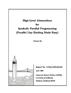
Current methodologies and productivity improvements are failing to keep pace with the rapid and ongoing increase in complexity and technology improvements [SIA97].

requiring the size of design teams or the numbers of hours they expend to increase at the same rate. At the remarkable rates of increase in circuit densities and gates per design, without such productivity amplifiers, organizations that attempt such designs would soon run up against the limits on managing ever-growing design teams, or at least the current limits on the number of trained professionals available in the workforce. This trend is shown in Figure 1.1, using data from the National Technology Roadmap for Semiconductors, 1997 [SIA97]. The need to improve productivity leads the way in stimulating innovation in hardware synthesis methods, since it occurs at the leading edge of technology where demands and rewards are great but existing methods fail to serve for long without breaking down. The second driver of improvements in hardware synthesis is not at the high-end of complexity and performance, but at the broad-based low-end of seeking to make powerful integrated circuit technology available to a wider range of designers. Productivity amplifiers not only enable the biggest and best teams to go further, but also can allow smaller numbers of less 3

experienced individuals to have access to technology that was previously only an option for well-funded larger groups of trained specialists. A prime example of this second driver is in synthesis for FPGAs and other programmable devices, where entry costs are much lower since integrated circuit fabrication is not necessary, but the performance of the technology is still adequate for a wide range of applications. Designers with minimal knowledge of circuit design can produce designs implemented on programmable devices with satisfactory performance for simple and mid-range design complexities. This is the second-wave or “echo” benefit of all the efforts that have been expended on leading-edge problems. The majority of attention in hardware synthesis has focused on the most general case of random logic synthesis, where little can be assumed about either the variables and data types being manipulated, or about the flow of control during operation. With more knowledge of the structure of the applications of interest, a greater degree of specialization is possible. Digital signal processing (DSP) is the application domain where the greatest success has been achieved in creating specialized algorithms and tools for hardware synthesis. The DSP domain includes the areas of communications, speech synthesis and recognition, audio, image and video processing, sensing and imaging, data compression, and control systems. DSP applications are generally characterized as being dominated by numerical computations, as opposed to logic operations, and as being relatively limited in their control flow branching. Both of these properties make specialized methodologies for designing implementations of such systems practical. Such methodologies take advantage of the regularity in structure and control of DSP applications in order to achieve results of greater quality, and to do so in less time than would be possible by using general tools designed for random logic synthesis.

4

1.2

From Silicon Compilation to Electronic Design Automation

The general area of hardware synthesis comes under the broader field of electronic design automation (EDA). EDA deals with all aspects of non-manual approaches to the design of electronics. This ranges from the design of circuit layout geometry all the way up to the level of complete systems, including systems composed of both analog and digital integrated circuits, embedded software, and mechanical elements.

1.2.1

Origins

EDA has a history of more than 25 years, and is continuing to evolve and change. Many of the early ideas emerged in the 1970s, stimulated by the increasing availability of powerful mainframe and minicomputer systems to electronics designers [Yoffa97] and the increasingly complex demands of VLSI technology [Gray79] [Collett84]. Broad commercialization took place in the 1980s, with algorithms and tools coming from universities and private research laboratories into the electronics engineering market. Broad acceptance of EDA tools and methodologies has solidified during the 1990s, to the point that nearly no innovative electronic component or system can be designed in an economical way without the use of EDA methodologies. The revenue for the entire EDA industry in 1997 is estimated at over $2.70 billion, and continues to grow [Santarini98b]. One of the first uses of automation in electronics engineering was to assist the designer by alleviating some of the tedium of basic tasks such as schematic capture and logic simulation [Yoffa97]. This was termed computer-aided engineering or CAE. These tasks were essentially recording the designer’s intent, or computing the expected outcome of a deterministic model of their design. From this beginning, a new direction emerged where tools would be developed to make design decisions instead of just to capture and report on the outcome of designers’ decisions.

5

One of the early tasks to which automation methods were applied was artwork generation [VLSIStaff84b]. Artwork generation is the production of a geometric layout in polygons from which a circuit layout in silicon is manufactured. A researcher made a proposal at a Design Automation Conference (DAC) in the mid-1970s for a system that would generate artwork automatically from a human-readable description. An unknown attendee who saw this proposal characterized it as a silicon compiler, making an analogy with systems that produce machine instruction code from human-readable software descriptions [VLSIStaff84a]. Some of the earliest published work to refer to silicon compilation came at the 16th DAC in 1979, from authors associated with the Silicon Structures Project at the California Institute of Technology [Ayres79] [Gray79] [Johannsen79].

1.2.2

Silicon Compilers

The term silicon compiler does not have a strict definition, but rather it evokes a general concept that is easily grasped and retained by anyone familiar with software compilers. An early author defined silicon compilers as “programs which, when compiled, yield code that produces manufacturing data for silicon parts” [Gray79]. A similar definition is “an optimizing transformation program that produces manufacturable IC designs from intelligible descriptions” [VLSIStaff84a]. A more specific definition in terms of input and output is “a software system that accepts some form of high-level specification and produces a pattern-generation tape for the mask-making process” [VLSIStaff84a]. While the back-end output of a silicon compiler in the form of a pattern-generation tape or mask layout was often well-defined, the front-end to the process was less consistently defined [Panasuk84]. Different implementations accepted design input at the logic level, the block-diagram level, and the functional-description level [Southard84]. One definition that has the perspective of time, coming a decade after the first definitions, conveys the movement away from monolithic silicon compiler programs to sets of 6

individual tools in a flow. The LAGER silicon compiler toolset from UC Berkeley is described as being “composed of design managers, libraries, design tools, test generators and simulators, which are interfaced to a common database... Another major set of tools in LAGER involve using higher level descriptions of behavior to synthesize the structural description, which in turn is used to provide the necessary input data to the layout generators” [Brodersen92]. Early proponents of silicon compilers saw them as a way to address the design requirements of increasingly complex VLSI chips. The complexity possible in chip designs approaching one million transistors on a single chip was seen as precipitating a crisis in electronic design [Gajski84]. This crisis had two major elements, a shortage of trained chip designers, and an increasingly long design cycle. Designs of over 100,000 transistors were reported as requiring hundreds of staff-years to produce manually [Panasuk84]. Partial automation of the chip design process, through silicon compilation, was seen as a necessary way to address these issues. While early attempts at automation were acknowledged as producing sub-optimal designs in comparison to manual techniques, this was weighed against the need to increase productivity and shorten design cycles [Allerton84]. Similar gains were expected by those who had observed the advantages of compilation over manual coding and assembly in the software world [Ayres79]. Another significant motivation to move to silicon compilation was to reduce the increasing number and cost of errors occurring in the VLSI design process [Cheng84]. Perhaps the most inspiring motivation to researchers and others wishing to take advantage of powerful integrated circuit technology was the hope that silicon compilers would open up the field of chip design to system designers and end-users of VLSI circuits [Mead82] [Johnson84]. Early attempts at silicon compilers were pioneered at universities and larger private research laboratories. Among the university efforts were Bristle Blocks [Johannsen79] and 7

Siclops [Hedges82] from the California Institute of Technology, MacPitts from the MIT Lincoln Laboratory [Southard83] [Fox83], FIRST from the University of Edinburgh [Denyer83], DIADES from Warsaw Technical University [Wieclawski84], and ICEWATER from University of Waterloo [Powell83]. During the same period, commercial research laboratories were also working on silicon compilers and related tools. These included the Functional Design System (FDS) and PLEX from AT&T Bell Labs, the Xi Logic Generator from Bell Communications Research, the Design and Verification System (DAV) from IBM, as well as a separate Logic Synthesis System and Technology Mapping System from IBM, the ANGEL system from NTT, and the SILC silicon compiler from GTE Laboratories [VLSIStaff84a] [Ciesielski84]. Efforts to commercialize silicon compiler technology followed quickly. Some of these efforts came directly out of research and personnel from the universities and larger laboratories. Founders of Silicon Compilers, Inc. (SCI) came from Caltech’s Silicon Structures Project, including David Johannsen [Werner83b]. Work on Bristle Blocks was extended by SCI to create Genesil. Genesil found early success in use by Digital Equipment Corporation to design the datapath chip for the MicroVAX 1 in seven months [Collett84]. Researchers from MIT Lincoln Laboratory extended and commercialized the MacPitts system as MetaSyn when they founded Metalogic. Similarly, Silicon Design Labs was started by researchers from AT&T Bell Labs who had worked on the PLEX project. Other commercial efforts included cell compilers and chip composition tools from VLSI Technology, and Seattle Silicon Technology’s Concorde I system, which was incorporated into a larger design environment by Valid Logic [VLSIStaff84b].

8

1.2.3

Difficulties in Practice

These early efforts at silicon compilation attempted to automate significant stages in the design process. In later years, they did not prove to be the all-encompassing solutions that were originally hoped for [Yoffa97]. According to one observer [Perryman88], by 1988 the use of silicon compilers had not grown as much as had been predicted, and two-thirds of the original commercial vendors did not remain in the market. A number of reasons for this were cited, including the continued need for the use of manual design to achieve the highest performance designs. This was due to a lack of capability in the existing silicon compilers to allow experienced designers to achieve optimal solutions. Among a less experienced set of users, it was claimed that existing tools had too much complexity to allow novice designers to obtain suitable solutions. Therefore, silicon compilers had not realized two of the original goals intended for them: to increase the productivity of experienced designers without degrading the quality of results, and to open VLSI design to less experienced designers to create designs for their own use. Also cited was a lack of application-specific features in the common denominator silicon compilers that were available. Other observers noted a cultural resistance in the design community to adopt silicon compilation methodologies [Andrews88]. Silicon compilers were accepted as an alternative design tool, but not universally. These tools were not used for high-performance designs because evaluations did not show them to be capable of producing efficient designs. It was expected that as silicon compiler technology developed, this situation would improve. At the same time, many tools called for the use of high-level languages for design input instead of the then-familiar gate-level schematics and block diagrams. The use of expressive high-level languages was expected to allow more succinct specification of greater complexity, but experienced designers and managers were not accustomed to this new style. 9

One problem was the multitude of languages that were put forward by individual vendors with no common standard. As is discussed in the next section, both de facto and official standards eventually emerged that drew a critical mass of designers, leading to the widespread adoption of high-level language specification as design input. Another problem was dissatisfaction with monolithic silicon compiler tools that didn’t allow customization of the design process as new requirements emerged, such as test generation, or that users found the need to become involved with manually adjusting the final layout in order to achieve satisfactory results [Goering88]. These needs led to the fragmentation of the silicon compiler into multiple specialized tools joined by design flows and frameworks, as is described in a later section below.

1.2.4

Languages

Early silicon compilers allowed for various styles of design specification input, since there were no broadly accepted standards other than boolean logic. Some compilers were conceived as transforming a designer-specified architecture or structure at an abstract level, such as a block diagram, into a gate-level and layout-level structure with the structural topology preserved, but details elaborated and filled in within each block automatically. Other compilers were patterned after software compilers, taking in a specification in a text language form and determining a structural representation from the text specification. A variety of input styles were used by early silicon compilers in research and in commercial offerings, including graphical block diagram editors, textual languages, forms, tables, and combinations of these. Among the graphical methods, drawing schematics at the logic gate level was supported by many tools, but was a lengthy process for designs of more than a few thousand gates [Beedie84]. Menu-based approaches that would allow the selection of predefined components from hierarchically-grouped lists were used by the 10

Concorde I silicon compiler from Seattle Silicon Technology [Lee84]. Some tools also used finite state diagram editors to allow the specification of control flow. Among tools that allowed text input, logic equations were a natural and standard choice, but were also limited in the way that gate-level design entry was. The MetaSyn silicon compiler, which was MetaLogic’s commercial version of the MacPitts compiler, used a textual input language based on LISP [Southard84]. Other text-input languages for silicon compilers included ICL from Xerox [Ayres79], LISA, an instruction-set language from the University of Illinois [Gajski82], VIP from VLSI Technology [Martinez84], ZEUS from GTE Laboratories [Nourani84], SCHOLAR from the University of Southampton [Allerton84], as well as MODEL from Lattice Logic, ELLA from the Royal Signals and Radar Establishment of England, and STRICT from the University of Newcastle, England [Beedie84]. Another style of design entry, forms, was used by the Genesil silicon compiler from Silicon Compilers [Johnson84]. Standard blocks such as ALUs, barrel shifters, RAMs, ROMs, and random logic could be selected, and specific parameters and connections specified for an instance using data entry into fields in a form. The system would provide feedback to the user by updating a graphical display of the blocks and connections, but this display could not be directly modified by the user. Still other formats for design entry were tabular, using truth tables for combinational logic and state transition tables for sequential logic representations. It is possible to represent a structure in both a text form and in a block diagram form. It is also possible to describe an abstract behavior in either text or a block diagram, and to transform it into one of many equivalent structures from which the final circuit layout structure is elaborated. There was disagreement over the choice of text or block diagram input styles [Werner83a]. Text specifications were favored by software developers accustomed to text languages, who were also working on computing platforms that were adept 11

at manipulating text representations. Block diagram specifications were preferred by many circuit and system designers who were accustomed to drawing and interpreting block diagrams, gate-, transistor-, and layout-schematics. While it is possible to represent either behavior or structure in either text or a block diagram, text was usually associated with behavioral descriptions and block diagrams were associated with structural descriptions. Some felt that it was a mistake to start from a behavioral description and allow the silicon compiler to determine an architectural structure because it would prevent designers from using their skills in designing architectures. Others felt that there were opportunities to be realized by starting with an abstract behavior that was not limited by initial assumptions about the eventual architecture [Werner83a]. The initial stage of this latter class of problem, determining an architecture from a behavior, eventually came to be called behavioral synthesis, architectural synthesis, or frequently high-level synthesis. Behavioral synthesis is discussed further in later sections below. One factor that inhibited the early development of behavioral synthesis was the lack of intermediate structural specification languages. A number of languages were created for specific tools, but no common, accepted languages were available from which to build a body of design work across design tools. Also, because the behavioral synthesis problem adds additional complexity to the overall design automation problem, most early silicon compilers either used simplified transformations from behavior to an unoptimized architecture, or they avoided the problem by beginning with architecture or gate-level design as the specification input. While a wide range of input specifications were used by the various tools available, some observed that ultimately, the more expressive specification languages would allow for greater productivity. Some asserted that for more than a few thousand gates of complexity, higher-level descriptions were called for [Beedie84]. Not all designers reached the point of working at or above that level of complexity at the same time. Some of the first to do so were likely to be among the more experienced designers. These very designers 12

would be less likely to adopt design automation methods for two reasons. First, they were experienced and long accustomed to using manual techniques. Second, they were often skilled enough to produce designs of higher quality than the early EDA tools could. These factors delayed the widespread adoption of language-input methodologies, but that change did eventually take place, especially when many designers moved to the register level of design specification. One tool that emerged in 1988 to focus on a particular stage in silicon compilation, that of optimized logic synthesis, was the Design Compiler from Synopsys [Weiss88]. The first version of this tool allowed design entry in netlist formats, logic equations, and truth tables. A year later, the tool was extended with a front-end that would allow the use of subsets of Verilog and VHDL (described below) as design specification inputs [McLeod89]. In retrospect, Aart de Geus, the CEO of Synopsys, observed that as the majority of designers moved from the scale of 1,000 gates to 10,000 gates, roughly between 1988-1990, schematic entry as an input became too cumbersome, hastening the adoption of languagebased design input [Glover98]. Some early proponents of silicon compilers urged the adoption of high-level languages known in the software world as input descriptions for electronic design, including FORTRAN, C, Pascal, and LISP. Since these languages were already widely known, there would be a larger base of designers who would not need to learn a new language in order to use electronic design automation tools. These languages either proved to be too expressive for hardware design, because they permitted dynamic memory allocation or had datadependent computation requirements, or not expressive enough, because they did not support the specifications of timing, data precision, or concurrency that designers wished to have. Some of the languages used for early silicon compilers were inspired by these software languages, but were always taken from a subset of the original language or augmented in some way to fit the methodology being used. 13

Rather than deriving subsets of or extensions to existing high-level languages, the languages that were designed directly for the description of digital hardware systems proved to be more successful. These languages directly supported hardware design constructs such as logic, data registers, signals, hierarchy, and synchronous clocking. These languages are called hardware description languages (HDLs). Two of these that eventually emerged as dominant were Verilog and VHDL, displacing many of the early languages fashioned for use in electronic design automation. Verilog started as a proprietary HDL designed for simulation. It was developed by Gateway Design Automation for use in a simulator product. While Verilog was proprietary, it came to be widely used in industry for hardware simulation. Due to its popularity, it was chosen by Synopsys as an input language for their Design Compiler tool, extending the use of the language from simulation to logic synthesis. In 1989, Gateway Design Automation was purchased by Cadence Design Systems, which continued to market the language for simulation and synthesis. In 1990, Cadence moved Verilog into the public domain, and in 1995, Verilog was made IEEE Standard 1364 [Dorsch95]. VHDL began in 1983 as a U.S. Department of Defense (DoD) initiative to create a text-based language for specifying digital hardware designs (See Chapter 3). The language was later extended to support simulation, and was released as IEEE Standard 1076 in 1987. VHDL was adopted along with Verilog by Synopsys when it created an HDL frontend to Design Compiler. VHDL also increased in popularity due to its earlier adoption as an international standard. Both languages were suitable for both simulation and synthesis, and both became standardized and widely supported by EDA tool vendors. The languages have broad semantics which are comparable enough that neither emerged as having a distinct advantage in use over the other. As a result, both VHDL and Verilog continue to be widely used and sup-

14

ported internationally, a situation which some observers have lamented as being redundant and costly for both tool users and tool developers [Dorsch95]. In practice, neither VHDL nor Verilog are used in standard form as inputs to synthesis methodologies. Because of their origins as languages for general digital system simulation, their semantics are too broad to be used in their entirety for synthesis. In order to make the languages appropriate for synthesis, subsets of the languages are defined which are acceptable to each synthesis tool as input. Often as a result, the accepted subset for each synthesis tool is distinct from the others, which results in a loss of the standardization which was defined for the full languages. This is true of both register-transfer level logic synthesis and behavioral synthesis, which are described in later sections. Various efforts to standardize synthesizable subsets of VHDL and Verilog have been proposed, and are standards are continuing to be defined.

1.2.5

From Compilers to Frameworks

Even with the partial success of silicon compilers, they did not prove to be complete solutions [Yoffa97]. One reason for this was that silicon compilers focused only on the design problem between the structural level of specification down to the physical level of the generation of layout data. Other tools were needed to handle such design tasks as system-level design from the behavioral level down to the structural level, simulation, timing analysis, standard-cell library creation, and design rule checking. Another reason was that silicon compilers kept their part of the design process closed, from design entry down to the layout, with little opportunity for designer intervention at stages along the way. The first problem was essentially that individual design tools covered a well-defined but limited scope of the process. Many tools were developed to cover different design problems, and tools tended to have differing data formats for input and output. Just as there had been difficulties with the many languages created for design specification, other 15

interchange formats were also incompatible. Katz identified this emerging problem, and suggested that the way to move from loose collections of non-interoperable tools to truly useful design systems was to develop standardized integrated design databases [Katz83]. Another means of addressing the need for tool interoperability was that either “de facto” or official standards would arise out of a set of competing specification formats, as eventually happened with Verilog before it became standardized, and before VHDL was officially introduced. Standards such as the Caltech Intermediate Format (CIF) for geometric circuit layout data [Mead80] and the Electronic Design Interchange Format (EDIF) for general design data exchange [Eurich90] are also in the pattern of de facto standards being followed by official standards. The second problem, that silicon compilers were usually closed systems within the segment of the design flow that they covered, was an issue for designers who wished to be able to observe more detail or to have more control of the design process at intermediate points in the flow. Another hindrance to the acceptance of monolithic silicon compilation tools was that designers wished to mix-and-match smaller, specialized tools to create their own customized design systems suited to their particular needs. As the number of tools available from various vendors increased, such as for schematic capture, logic synthesis, test generation, layout, design rule checking, and verification, more designers wished to be able to select what they perceived as the best of each from those vendors that excelled at different types of tools. No one silicon compilation tool was seen as being preferred in all aspects of design, which restricted their acceptance. The trend toward CAD frameworks [vanDerWolf94] instead of monolithic tools was served by companies such as Valid Logic Systems and Mentor Graphics that offered integrated sets of tools. Existing silicon compiler tool vendors, such as Silicon Compiler Systems, were not as successful with their tools, and

16

responded by unbundling their products into sets of tools that could work within a single framework [Weiss89a]. While individual vendors produced and sold their own frameworks, this was not enough to allow interoperability among tools from different vendors. A further move by vendors to freely provide open interfaces to their design frameworks was intended to promote third-party tool development and integration with frameworks [Wirbel89] [Harding89]. The arrival of VHDL during the same time period as a standard, mandated for use by the U.S. Department of Defense, led many tool developers to support VHDL as a common standard for design interchange among tools [Harding89] [Weiss89b]. An industry-sponsored collaboration began in 1988, called the CAD Framework Initiative (CFI) [Harding88] to address problems of design data exchange and tool interoperability. While these and other industry and research efforts continued through the mid 1990s, standards for tool integration were not widely adopted by tool vendors, partly due to the competitive rivalries of EDA vendors, and the lack of any one vendor being dominant enough and willing to set a standard that others would follow [Shneider91]. It is not necessarily in commercial EDA vendors’ self-interest to make their tools fully interoperable with those of other vendors, despite the difficulties that designers have due to noninteroperability. In 1997, the CFI announced that it was changing its name to the Silicon Integration Initiative (SI2), and that its focus would shift to improving productivity and reducing the costs of designing and manufacturing integrated silicon systems [CFI97]. Tool interoperability continues to be a problem. One figure quoted is that up to 50% of semiconductor companies’ design tools groups resources are spent on integrating tools together [Goering98].

17

1.2.6

Mainstream EDA

With the passing of monolithic silicon compilers to sets of tools and frameworks, the term silicon compiler fell into disuse, but has not disappeared completely. Recently, the term is used only to refer to systems that take a description of the structure of an application or function and perform all of the steps to produce a layout. This approach is typically restricted to special domains, such as filter design within DSP [Miyazaki93] [Jeng93] [Hawley96] and fuzzy logic [Wicks95] [Manaresi96], where domain-specific knowledge can lead to optimal rules for efficient layout. For general digital system design, the term appears to be rarely used. The basic steps that were performed by the first silicon compilers are now performed by many tools joined together in a design flow. The Design Compiler from Synopsys is not a silicon compiler at all, since it only performs logic synthesis, but performs no layout functions. Many other tools have arisen to handle specific tasks required by designers, and each task is referred to by separate names. In addition, the design process is not thought of as a monolithic, turnkey process where even an organized set of tools can handle the many steps of circuit layout design without interactive control from designers. The general field of design tools, frameworks, and services falls under the term of electronic design automation (EDA). During the past few years, EDA tools have become mainstream in their use and somewhat indispensable for creating innovative designs in a cost-effective manner. Logic synthesis has taken hold as a crucial step in many design flows, and it has been improved and extended to take more into account about the technologies to which it is targetted, be they full-custom layout in a given silicon technology, standard-cell design, gate-array, or FPGA implementations. In addition, sub-specializations of logic synthesis are sometimes used for control logic and datapath design. For control, sequential logic optimization of state machines is a specialized area within logic synthesis. For arithmetic operations and signal

18

processing, datapath compilers are emerging as additional tools to work with logic synthesis. Other tools within digital design flows include tools for physical design. Among these are tools for floorplanning prior to the final layout, to improve the eventual layout results and to improve logic synthesis by providing early estimates of delay and area from the layout. Tools for placement and routing also continue to grow in sophistication as silicon technologies become more challenging to design for. Parametric extraction of parasitic resistance and capacitance are used to achieve more accurate estimates of delay and power consumption from the layout, and design rule checkers to verify that layout rules have been followed are also crucial to avoid expensive layout redesigns after failed fabrication. Other tools at the layout level support the design of standard cell libraries and their characterization so that libraries can be targeted by logic synthesis. Design for test and design for low power are also motivations which are changing and extending the capabilities of logic synthesis tools. Simulation tools at all levels of design have become important for informal verification of designs and to check for errors created in moving from one level to another. Above the level of logic synthesis, tools for analyzing source HDL code help designers to target areas of source code that lead to specific problems in synthesis by annotating the code with synthesis results. Other tools aim at design levels above logic and register-transfer-level synthesis, including behavioral synthesis (described below) and emerging tools for hardware-software codesign and system-level design. System integration standards for the design of systems-on-a-chip (SoC) are being put forward by industry-sponsored groups such as the Virtual Socket Interface Alliance (VSI Alliance). These efforts are intended to promote the level of design to the system level for complex integrated circuits, and to allow the re-use of components in multiple IC designs.

19

Behavioral synthesis (described further in Section 1.5) takes a behavioral specification as input and produces a register-transfer-level (RTL) design for input to RTL synthesis. A behavioral description does not specify specific timing or functional unit allocation, but only the operations to be performed and their dependencies upon one another, along with timing constraints on the eventual implementation. Behavioral synthesis represents the highest level of abstraction at which some early design tools worked, and serves as a frontend to the remainder of the design flow. Behavioral synthesis tools were successfully commercialized after RTL synthesis tools had become accepted. Mentor Graphics adopted the Cathedral tools from IMEC as the Mistral system for DSP circuit design. These tools carried specific assumptions about the architecture with them. A general tool for behavioral synthesis was introduced by Synopsys in 1994, Behavioral Compiler, which was presented as not being appropriate for all design styles, but rather for algorithmic design. In 1997, the Alta Group of Cadence Design Systems released Visual Architect, a behavioral synthesis tool with an interactive interface presenting multiple views of the behavioral synthesis process. A tool containing similar capabilities called Monet was introduced by Mentor Graphics later in 1997. Synopsys later introduced BCView, a visual interface extension to Behavioral Compiler. Behavioral synthesis tools in general are not always appropriate for general designs, but find their best use for designs with high algorithmic content, such as for DSP and arithmetic datapath design.

1.2.7

Emerging Challenges

The long-term trend in the industry has been to move from single all-encompassing tools to multiple tools in a design flow. Some of these tools have emerged from research work at universities and larger private research laboratories. Products are commercialized, sometimes by the existing major EDA vendors, and just as often by smaller startup companies. Multiple entrants to the market appear initially, followed by a few emerging as domi20

nant after a few years. Often, consolidation through attrition of weaker product offerings and large EDA vendors’ mergers with and acquisitions of smaller successful startups is a pattern which repeats itself with each new wave of EDA technology. While innovation in the past used to be led by non-EDA industry research efforts, followed by commercialization, recently much innovation comes incrementally from industry itself. Often these incremental advances are additional features within existing design tools, or new tools which fit into existing design tool flows. Some recent areas of innovation are design for low power, design for test, verification, system-level integration, and layout-level tools to deal with the challenges of deep-submicron (DSM) scale technology. While many design tools are being modified to handle design technology down to 0.25 microns in scale, a large question in the industry is how to deal with technology at smaller scales, where many of the assumptions and typical design abstractions break down. One issue involves the fact that as logic elements shrink, the dominant contribution to circuit delay, area, and power consumption comes from the interconnect and not from the transistors. Another issue is that transmission-line effects and crosstalk among interconnect traces becomes increasingly difficult to avoid. Some are calling for an entirely new design flow below the RTL abstraction in order to meet these challenges, while efforts still continue to modify existing flows incrementally to adapt to shrinking technology scales. A likely feature of new design flows would be the tighter coupling of logic synthesis, floorplanning, and place & route, instead of treating each of these as separate stages. For datapath-intensive designs, the possibility exists for the return of earlier silicon compilation techniques [Goering97a], where automation is applied from the behavioral or structural description of datapath sections down through the final layout. Because of the regularity of datapath designs in their layout, silicon compilation has proven its greatest value, over general logic synthesis and layout, in this area. The challenges of DSM-scale 21

designs makes this option more attractive to designers who are not expert in manual datapath design. With DSM, less emphasis may be placed on reducing the overall number of gates, and more importance may be assigned to obtaining layouts with predictable performance, area, power requirements, and signal integrity. One of the early silicon compilation techniques was applied by VLSI Technology for standard-cell layout of datapaths. DSP is one of the areas where silicon compilation has been most successfully applied, in tools such as LAGER [Brodersen92] and others [Miyazaki93] [Jeng93] [Hawley96]. Recent commercial product offerings that address datapath design at various levels include the Smartpath layout tool from Cadence Design Systems, which provides automated layout of data-path elements (1995), the Mustang datapath placement tool from Arcadia Design Systems (1996), the Aquarius-DP datapath-placement tool from Avant! (1997), and the Datapath Compiler tool from Synopsys for automatically synthesizing structural descriptions of datapath elements into gates (1997). Even with these developments, large companies with many resources will likely continue to design high-performance datapaths for leading-edge microprocessors by hand, since obtaining the greatest possible performance from the datapath is central to the success of these products. Going forward, the challenges of designing systems in integrated circuit technology lie both in the difficulties of working in shrinking DSM scales, as well as the desire to increase productivity through raising the abstraction level where appropriate and making greater re-use of existing designs. Just as the coming of VLSI design was seen as precipitating a design crisis, today after several generations of technology and orders of magnitude in Moore’s Law, a crisis is being warned of in both the fine-scale of silicon technology and in large-scale system design productivity. Judging from the past, rather than halting progress, this crucial set of circumstances is more likely to spur greater efforts

22

Algorithm description: general requirements, mathematical equations, procedures, graphs, constraints code generation Behavioral Description: behavioral HDL code, high-level language behavioral synthesis RTL Description: RTL HDL code rtl synthesis Logic Gate Netlist technology mapping Technology-mapped netlist place and route Placed and routed netlist layout Layout: Semiconductor process mask images fabrication Implementation: Fabricated integrated circuit Figure 1.2

A typical design flow.

at innovation, and greater willingness to embrace new approaches derived from that innovation.

1.3

Levels of Abstraction

The fundamental implementation technology of semiconductor materials is far too basic for direct translation from an algorithmic specification to be reasonable. Instead, several successive layers of refinement in abstraction are passed through on the way from algorithm to implementation. These are presented in Figure 1.2 in a typical vertical design 23

flow, with the most abstract being at the top and the concrete physical implementation at the bottom. This is meant to be a general representation of a design flow, not an all-inclusive one, and it is not necessary to traverse it sequentially in top-to-bottom fashion. There are typically many iterations between levels of abstraction, including branching of design alternatives, as well as partial refinement of designs at mixed levels of abstraction [Hadley92]. There are also methodologies in which skipping levels of abstraction in the design flow is appropriate. The lowest levels are the most well-defined and standardized according to the current technologies available. The upper levels are less well-defined and have more available alternatives for how designs are specified at those levels of abstraction. The focus of this dissertation is on the top levels of this design flow, from the algorithm description to the RTL description of the design. At the top level, the algorithm description is the most open-ended since it can be defined as including all design descriptions that are more abstract than those that lie below it. Algorithms may be specified in terms of constraints or mathematical equations in variables of interest that may or may not be in closed-form expressions. An algorithm may also be specified in terms of a procedure or sequence of steps which describe the manipulation of abstract data structures, with control flow for specifying constructs such as decisions, iterations, branching, and recursion. Algorithms may also be specified in terms of graphs of abstract objects and the relationships among them. The term behavioral description has a more standardized meaning in hardware synthesis. It refers to any description that expresses the operations that are to take place and the communication of information among them, without specifying the allocation of resources to accomplish those operations or communications, and without specifying the exact timing of those operations or communications, either in their starting times, their durations, or their total ordering. Behavioral descriptions are a subset of algorithmic descriptions, since 24

they specify operations and their relationships explicitly. Algorithmic descriptions may or may not completely describe the specific steps to accomplish the desired goal, specifying instead only implicitly through a set of constraints or as a general procedure without a complete definition of the data structures or precise operations that bring about the goal. The register-transfer level (RTL) of abstraction can be defined in terms of what is not present in the behavioral description. An RTL description contains information about all the operations and communications present in the system, including specific information about which resources are instantiated to perform those operations and communications. Among the information included are statements of what registers, or data storage elements, are present and how and when they are to be used to store the results of operations, and to transfer those results to subsequent operations that use those results. An RTL description may not explicitly describe when all operations in the execution of the system take place, but it will completely describe the preconditions for all operations, possibly in terms of logic operations on signals which are within the system or which are inputs to the system from the environment. The timing of the loading of registers is described in terms of one or more clock signals. These clocks may or may not be synchronized to one another and their frequencies need not be specified in the RTL description.

1.4

RTL Synthesis

Once a valid RTL description of a design is available, it can be directly translated into a netlist of digital logic gates. This neglects, for the moment, whether or not the gate-level design will be feasible in any available semiconductor technology, as well as other issues that stem from physical properties of the technology. It is also possible to perform optimizations during translation from RTL to a gate-level description, but these will not change global timing or the data types or the allocation of registers.

25

RTL synthesis proceeds by a parsing of the RTL description to determine what registers, arithmetic operators, logic elements, and switching elements are instantiated. The synthesis process also determines from the RTL description what signals are connected between the previously mentioned elements, including input and output signals, and their bitwidths. Consistency checks are made for such conflicts as operator and signal bitwidth mismatches, or signals that appear to be driven by multiple source elements simultaneously. Once a consistent netlist of connected elements is ready, each of the elements can then be mapped to sub-netlists of connected logic gates. The choice of logic gates to use can be influenced by the implementation technology that the netlist will be mapped to. A logically correct netlist can be constructed by choosing any sub-nets of logic gates that implement the correct logic functions between registers. Such choices may not be optimal in terms of the goals of the design, and they may not even be feasible in terms of meeting the minimum requirements for size, performance, or power consumption, which are not specified in the RTL description. Pursuing the next step after RTL synthesis, technology mapping, can provide paths to predicting these design quality metrics. In technology mapping, alternative selections of logic gate sub-nets can be made depending on whether a specific standard library is being mapped to, or the selection can be determined by algorithms which optimize the design locally or globally in terms of area, switching delay, or power consumption. The inputs to such optimizations are estimates of the physical properties and behavior of the sub-nets in the final implementation technology. These estimates can come from characterizations of measurements which have been made on standard libraries of implementations of sub-nets, or standard cells, or they may be derived from models of the physical properties and behavior of sub-nets of logic gates in a given technology.

26

Any such optimizations will only be as good as the library and model estimates that are used as inputs. Increasingly, as deep-submicron (DSM) semiconductor technologies are chosen for the final implementation, the optimization algorithms must take into account less about the power, delay, and area of sub-nets of logic gates, and more about the same properties of the interconnections among them. Formerly, the majority of the area, delay and power consumption were due to the transistor circuit elements. This allowed general properties of a design to be determined from a netlist topology without placement information. For the increasingly shrinking technology scales of DSM, the majority of area, delay, and power consumption are due to the interconnections, and so are determined by the placement and routing of the interconnect. Since the sizes and geometries of interconnections are not specified in a netlist of technology-mapped logic gates, accurate predictions of power, delay, and area are increasingly difficult to obtain from such a netlist alone. Preliminary estimates from the next stage, placement and routing, may be required in order to estimate the geometries and physical properties of the interconnections. No matter what the final sub-net of logic gates that is chosen for each element in the overall netlist, it must not change the logic function as specified in the RTL description. Within that constraint, there are limited opportunities for optimization. However, if the original design intent is more general than what is in any single RTL description, then a methodology which uses a specification closer to that intent will not needlessly constrain the design flow. If the intent does not specify what operators are to be instantiated to accomplish the computation, or how many of each, or when they should execute, then an RTL description, which locks in choices for all of these, constrains the quality of the result beyond the original design intent. If instead the designer can capture the intent at a more abstract level, many different RTL descriptions may be possible which can implement that design intent. The result may 27

be a broader design search space, which could imply a longer design time. However, if the time required to input and debug the more general design specification is significantly shorter than that needed for an RTL description, the benefits are twofold. First, the overall design time may be shorter than if the initial design input were in RTL form. Second, as a result of starting from a more general description, lower cost or higher performance alternatives may be possible which would not have been from a fixed RTL starting point. Recoding from one RTL description to another for design improvement can be far more difficult, error-prone, and time consuming than generating both RTL descriptions from a single, more abstract statement of design intent which does not need to be modified. Any changes in an RTL description must be verified against the original intent, but an RTL description which is generated directly from that intent does not need to be as extensively verified. A behavioral description is one type of more general specification of design intent, and behavioral synthesis is the process of generating an RTL description from a behavioral description.

1.5

Behavioral Synthesis

In this section we take a more detailed look at behavioral synthesis, [McFarland90] which takes a behavioral description of a design and produces an RTL description, subject to some optimization criteria. Other terms which are used commonly in the literature include high-level synthesis, architectural synthesis, and behavioral compilation. This type of methodology has proven to be particularly successful for DSP applications, as opposed to general digital logic design, achieving productivity improvements of a factor of five over RTL synthesis methods, while maintaining or improving area and timing [Camposano96]. A behavioral description lacks specific instantiation of computation and communication elements, and does not specify the exact timing of operations. The pur-

28

pose of behavioral synthesis is to decide what the instantiations and interconnections should be, along with the clock timing, so that an RTL description can be produced for use in the remainder of the design flow. The behavioral description may be written in a procedural text form, as in sequential statements in a hardware description language (HDL) such as VHDL or Verilog. Behavioral descriptions can also be written in high-level programming languages such as C or FORTAN. None of these languages is ever used without some significant restrictions, however. Many constructs that are acceptable in the general standard form of these languages are not allowed by behavioral synthesis tools. Either these constructs do not conform to the “style” required by the tool, or they are inherently unsynthesizable constructs, such as absolute timing specifications, dynamic allocation/deallocation of storage elements, or pointer addressing modes. In the case of C, a simplified language with a similar syntax has been developed, with additional constructs included for purposes of hardware synthesis [DeMicheli90]. As an alternative to modifying existing high-level programming languages, or to inventing new all-purpose digital design languages, specialized languages such as Silage [Hilfinger85] for domain-specific application areas can also be employed. Silage was created specifically with digital signal processing in mind, providing constructs for specifying signals in a sample-based syntax. Silage also provides operators for specifying sample delays. Silage is an applicative language. It is single-assignment, so that variables represent mathematical quantities and not memory locations. The syntax of Silage is comparable to the way in which designers would specify DSP algorithms as relationships among signals through discrete-time difference equations. As a result, Silage is well-suited to specifying such systems. The original language design has been extended to support timing information, pragmatic directives, loops, and conditionals [Genin90].

29

With the availability of domain-specific languages for describing DSP designs comes the possibility of having domain-specific tools for synthesizing implementations. A set of tools which focus on taking Silage descriptions as the input to synthesis and then performing architectural synthesis and optimization based on distinct architectural styles is the Cathedral family (I through IV). These tools are based on joint work at IMEC, the ESAT Laboratory at K.U. Leuven, and Philips Research Labs [DeMan90]. The four architectural styles supported are hard-wired bit-serial datapaths, microcoded multiprocessors, cooperating bit-parallel datapaths, and regular arrays. These tools tend to focus on very high throughput (> 100Mops/sec) applications. Also, clustering and memory management are performed manually, and the complexity of the algorithm for synthesizing applicationspecific function units is high, particularly when synthesizing many functions into a single functional unit [Note91]. The synthesis phase has more utility when combined with a larger design tool, as in the case of PIRAMID, which uses Cathedral II for synthesizing sub-units, a separate Module Generation Environment (MGE) for generating detailed layouts of sub-blocks, along with timing and area information, and a FloorPlanning Environment (FPE) for general architecture floorplanning [VanMeerbergen90]. Just as synthesis tools optimized for particular architectural styles can hold a specific advantage, so can tools which are targeted at particular application areas. The PHIDEO compiler from Philips is aimed specifically at high-speed processing of video streams, such

as

what

is

required

for

high-definition

television

(HDTV)

systems

[VanMeerbergen92]. A special requirement for video applications is the large amount of buffer memory which needs to be managed. In order to address this, the PHIDEO compiler has as a major step the design of a multiport memory to serve the multiple processor units which are also designed within the tool. While textual languages are currently the most common form of input for behavioral synthesis methodologies, they are not the only form possible. Graphical descriptions can 30

contain all the relevant information necessary for behavioral synthesis, as can mixed graphical/textual descriptions. This seems even more natural in considering the fact that many behavioral synthesis tools proceed by producing an internal graphical form of the specification on which the algorithms for synthesis operate. The comfort of programmers with sequential text-based languages, along with the transitioning of designers accustomed to text-based RTL coding over to behavioral synthesis, are primary reasons for the continuing predominance of text-based behavioral synthesis methodologies. Behavioral synthesis proceeds by constructing an internal dependency graph from the input description. This dependency graph has as nodes each of the operations that are to be performed during the execution of the algorithm. The edges are directed arcs representing data values that are exchanged between operations. An edge flows from the operation node that is the source of the corresponding data item to the node of the operation that uses that data item as an input. The edge may branch if multiple downstream operations require the same input data item. An edge can have exactly one source node, or it may be an input to the system from the outside. An edge can have multiple destination nodes, including the case of being directed to an output of the system. If an edge has no destination nodes, then the data value that it represents is not needed, and it can be eliminated. If an operation node has no output edges, and the operation produces no meaningful side-effects, then it can be eliminated as well. Once the dependency graph has been constructed, the steps of scheduling, allocation, and mapping can be performed, either jointly or in any order desired. Scheduling involves taking untimed operations of the graph, including input and output events, and associating them with specific time intervals in the execution of the system. Input and output constraints, as well as allocation and assignment constraints, and performance requirements, will dictate some of the scheduling decisions for the design. Estimates of performance, including estimates of how long each type of operation takes in the expected implementa31

tion technology, will constrain the remaining possible scheduling decisions. If no feasible schedule is possible within the given timing constraints, then either a faster implementation technology must be selected, or the behavioral description must be redesigned. The behavioral description may be changed, perhaps to trade off robustness in the presence of noise or expected error performance for additional execution speed. During the scheduling process, the dependency graph is annotated with information about which operations are to take place during each time interval. This in turn places minimum constraints on the spatial dimension in terms of specifying operations which are executed concurrently, and hence minimum resource requirements in order to enable that level of concurrency. The allocation phase determines the spatial dimension of how many physical elements of each type are to be included in the implementation. For each operator type, behavioral synthesis must allocate at least as many operators of that type as the maximum number of such operations that are expected to be simultaneously scheduled during any time step. Allocation applies not only to arithmetic and logical operators but also to registers and other elements that handle the communication of values from one operator to the next. The allocation phase must ensure that there are sufficient numbers of each type of element to accomplish the computation in the expected number of time steps. Behavioral synthesis must also determine which scheduled operations should be executed on which allocated operators, and which scheduled communications should be handled by which allocated communication elements. This phase is referred to as mapping, or assignment. An arbitrary mapping will likely result in suboptimal results in terms of the system cost. This is because the final interconnections between operators are determined by the operations which those operators are to perform and where the inputs and outputs of those operations are coming from and going to. The greater the number of source and destination elements for each operator, the more complicated the interconnect into and out of those 32

operators will be. In cases where interconnection paths between operators can be re-used by mappings of multiple dependency graph edges, additional interconnect need not be built. The result of the mapping phase is a design netlist which specifies all of the elements that need to be instantiated and their interconnections, as well as the timing of operations and the switching of data from one element to the next. Control signals which actuate the latching of registers and the setting of switching elements are derived from the input clock signals. From this body of information, a complete RTL description can be produced in the target language to be used as input to the RTL synthesis tool downstream in the design flow. Multiple such RTL descriptions can be generated through several iterations of behavioral synthesis, each performed with varied settings of the synthesis objectives and constraints. Each of these RTL descriptions will be a valid representation of the behavioral description intent without the need to manually re-code the RTL each time. The three phases of scheduling, allocation, and mapping need not be performed in any specific order. In resource-constrained scheduling, the allocation phase is performed first, setting strict limits on how many physical resources will be available so as to seek to put a cap on the implementation area. The scheduling which follows this will be subject not only to the dependency graph of the algorithm, but to the need to avoid scheduling more operations of a given type in a single time frame than there are operators allocated for that type of operation. This constrained optimization problem has been shown to be NP complete [Garey79]. Another variation on the three-phase ordering is partial mapping, where certain operations are pre-designated to be performed by specific limited resources, such as a special-purpose FFT engine. In this case, all other operations are unconstrained as to their mappings, but the overall design must remain consistent with the initial conditions specified for the mapped operations.

33

The three phases also need not be performed in isolation, where for example all scheduling is completed before any allocation or mapping can begin. Scheduling and allocation can be performed jointly. This can significantly complicate the algorithms required to perform these steps, but the hope is that superior results may be obtainable this way. An example of this is resource-constrained scheduling where the resource limits are not hard. If during scheduling it is found that the currently set limits from allocation are causing a particularly acute resource conflict, there may be limited flexibility to allow a slight increase in the allocated numbers of resources to resolve the conflict. Following this, the remainder of scheduling can continue under the new resource limits. Another important area of work that applies to behavioral synthesis even before scheduling, allocation, or mapping occur is the optimization of the input specification. Just as improved results have been obtained through the rewriting or transformation of the RTL code that is input to RTL synthesis, optimizations of behavioral specifications can enable better quality designs to be discovered. Transformations applied to the flow graph can lead to simpler or more regular flow graphs that will yield better results in behavioral synthesis. While work in this area has been in existence at the research level for some time, transformational approaches to optimization of behavioral synthesis have yet to be fully utilized in the currently available commercial behavioral synthesis tools.

1.6

Limitations of Behavioral Synthesis

Contemporary techniques for behavioral synthesis continue to face some limitations, which this research seeks to address in part. Methods which attack various portions of the scheduling/allocation/mapping problem for applications specified by dataflow graphs identify themselves as falling under the umbrella term “high-level synthesis.” However, when they are examined closely, they typically involve operations on graphical descrip-

34

tions of algorithms at the most primitive arithmetic level of task node granularity. The nodes are usually additions and multiplications, with variations allowed, perhaps, for multiple bitwidths within a single graph. Other work includes examples with arithmetic shifts and other functions defined by single primitive unary and binary operators. While this level of granularity may be convenient for the behavioral synthesis algorithms to attack, it is far below the level of specification at which designers of algorithms typically work, in that it does not include truly high-level operations such as filtering, frequency-time transforms, trigonometric functions, and encoder/decoders. One way to deal with this limitation of typical methods is to resolve high-level operations down into their constituent arithmetic operations, and so expand a graph of coarse-grain task node complexity into a much larger (in terms of the numbers of nodes and edges) graph of fine-grain complexity. What is gained is that the new graph representation more closely matches the kind of input specification which many behavioral synthesis algorithms are expecting. This type of approach has been applied with success in the area of software compiler design, where a similar fine-grain graph is used internally on which the algorithms operate. This works well for compilers that are targeting sequential machines, because the sequential nature restricts the complexity of this approach to software compilation. The significant drawback of this approach in hardware synthesis is that due to the parallel nature of the target implementations, many such synthesis algorithms are highly sensitive in their computational complexity to the size of the input graph specification. As a result, such algorithms are likely to require very long execution times to arrive at synthesis results when the entire fine-grain algorithm graph is used as input. In order to mitigate this problem, the fine-grain graph is usually broken into many smaller sub-graphs which represent portions of the overall application. The synthesis algorithms will find such smaller graphs to be much more reasonable in terms of synthesis time. This is similar to work done by [Lagnese91] for partitioning control-dataflow graphs 35

for various design goals prior to input to behavioral synthesis. Sub-clusters formed between partitioning boundaries are synthesized separately in their approach. A drawback to this method is that opportunities for optimizing resource sharing across the entire application are lost once the partition boundaries are drawn. The partitioning must strive to avoid cutting off valuable opportunities for resource sharing, but partitioning algorithms are limited by computational complexity in ways similar to how behavioral synthesis algorithms are. The result is that approximation heuristics must be applied in partitioning and clustering. Rather than first resolving an application graph down into fine-grain operations and then re-clustering it into multiple partitions to be sub-synthesized, we are interested in using the initial high-level graph structure to make informed resource sharing decisions. If a graph contains multiple coarse-grain operations which are similar, or identical, then that information can be of high value in discovering opportunities for resource sharing. Such information is lost if those coarse-grain operations are broken down into their constituent arithmetic-level operations. In order to re-infer that high-level structure from the low-level graph of arithmetic operations, sophisticated techniques in graph pattern-matching or clustering would need to be applied. There have been efforts in applying template-matching to behavioral synthesis [Corazao96] but such matching is limited to cases such as pairings of multiply-add operators or recognizing that subtractions can be implemented by adders and so be covered by adder templates. These bottom-up clustering techniques are aimed at small clusters, not the larger ones implied by coarse-grain operations of a larger scale. Another related effort by Potkonjak and Wolf [Potkonjak95] applied clustering to sets of individual tasks in order to minimize overall circuit area. This work, however, treated the tasks as separate and not sharing any data dependencies. The only stated goal was to attempt to minimize the area without any scheduling constraints among the tasks. In this

36

work we are concerned with minimizing area in implementing a full graph of tasks with data-dependency relationships. With a coarse-grain application graph, it is not necessary to have exact matching in operations in order for resource sharing to be deemed worthwhile. As an example, filtering operations where the realization type may be the same, but the number of taps differ can be implemented by a single section of synthesized hardware, provided that the filtering operations can be scheduled to take place at non-overlapping time intervals. Even significantly differing operations may be candidates for mapping onto the same synthesized hardware unit if such resource sharing will reduce the cost function while not violating the timing constraints. A further benefit of working with a coarse-grain graph comes from the reduced complexity in numbers of nodes and edges. With graphs of lower complexity, graph algorithms for synthesis can be accomplished more quickly, and a wider range of design options may be explored in the amount of time it would take to synthesize once from a large fine-grain graph of the same application. This is of course subject to the relative time cost of the algorithms used to synthesize the realizations of the large-grain clusterings as compared to the time cost of fine-grain clustering and behavioral synthesis. Also, because techniques that cluster from fine-grain graphs tend to group connected graph nodes together, they have a tendency not to favor clusterings of operations from disparate parts of the graph. Our proposed technique, which looks beyond local arithmetic connectivity, may explore clusterings which would not be typical for conventional methods to admit. This class of techniques may also prove useful for attacking problems of reconfigurable computing. This would apply to application specifications where large portions of the dataflow graph remain unchanged, but certain subsections change depending on decisions that are based on environmental factors, user input, or changing power and performance requirements. A single hardware realization may be required to implement multiple 37

such dataflow graphs. For the subgraphs of the dataflow graphs that embody the changes, hardware units can be synthesized which are capable of performing a few different node functions. Then these different functions can be selected by control inputs as reconfigurations take place during operation. In order to achieve similar results from behavioral synthesis at a fine-grain level, a single fine-grain graph representing all the configurations would need to be constructed. The reconfigurable portions could be isolated, but it would still be true that as reconfigurability demands increased, the complexity of the fine-grain graph would increase rapidly, significantly complicating conventional behavioral synthesis. With coarse-grain methods, we can now view hardware more flexibly as collections of concurrent functional units, each of which are operated sequentially, and which can be idled when not needed. Such hardware units can be marshalled into service as conditions change and then allowed to idle or shut down when not needed, saving power. A centrallyscheduled controller will always be active in organizing the available hardware units and interconnect resources as needs change. This controller will likely be significantly simpler if it only needs to actuate control signals for a few hardware units instead of for a large number of arithmetic operators and interconnect resources.

1.7

Summary

With multiple levels of abstraction available to hardware design specifiers and multiple tools from which to choose, each may be valuable under the right circumstances. For designs specified in dataflow, some form of behavioral synthesis approach appears appropriate, but most are aimed at a fine-grain representation of the design problem. By focusing on coarse-grain approaches, there is an opportunity to reduce computational

38

complexity and to discover design tradeoffs which might be difficult to infer from existing behavioral synthesis approaches. In the chapters that follow, we will describe such an approach, its strengths, and its limitations. We will also present techniques to make the approach interactive, and to allow verification through simulation with other non-hardware design elements. In Chapter 2, we present the details of a method for synthesizing hardware from SDF descriptions. In Chapter 3, we present issues in cosimulation of dataflow implemented in VHDL with other design elements. In Chapter 4, we describe how this design methodology can benefit from the use of interactive tools, and what the features of those tools should be. In Chapter 5, we present the details of how the synthesis, cosimulation, and interactive design procedures are implemented in the Ptolemy simulation and prototyping environment. Finally, in Chapter 6, we summarize the results of the earlier chapters and discuss open areas for future work.

39

2 SDF Hardware Synthesis

Synchronous Dataflow (SDF) is a model of computation well suited to represent applications with high algorithmic content, particularly multirate DSP. The features of SDF that make it useful as an initial specification from which to synthesize are the ability to perform static scheduling and the analysis of resource needs that is possible. From any SDF graph there are many possible implementations, and the issues involved are discussed in this chapter. In Section 2.1 we describe the SDF model, followed by an overview of SDF scheduling in Section 2.2. In Section 2.3, we discuss the dependency graph that is derived from an SDF specification. In Section 2.4, elements of the VHDL hardware description language are presented with aspects of how the dependency graph is representable in VHDL. Related work on constructing hardware from dataflow graphs is presented in Section 2.5. In Section 2.6, issues of implementing computation, communication, and control in a hardware architecture are explored. In Section 2.7, details of the communicationdriven style of implementation are presented. In Section 2.8 the stages of the code generation process are described. In Section 2.9 the hardware synthesis design flow is presented, followed by a summary in Section 2.10.

40

1

1 B 1

1 A

D 2

2 C 1

Figure 2.1

2.1

1

An example of an SDF system. Rates of token production and consumption are fixed for all actor firings, and are an explicit part of the specification.

Elements of Synchronous Dataflow

An algorithm specified in synchronous dataflow (SDF) represents a division of the total design into computation elements and their relationships with one another. As a graphical specification, it conveys not only which stages of the algorithm depend upon which others, but also it implicitly represents which stages are independent of each other. This shapes the direction in which the design of concurrently executing hardware units will go, determining which tasks can be performed by independent hardware units operating simultaneously, and which tasks must be performed sequentially. An SDF graph specifies the relative rates of production and consumption of data tokens for each firing of each actor. Given this, it is always possible to determine whether the graph is balanced, which means that it can be executed indefinitely with no unbounded accumulation of tokens on any of its arcs. It is also always possible to determine whether such a graph can be executed without deadlock. Deadlock occurs when no node can be fired because none has sufficient input tokens to satisfy the firing rules. An SDF graph that is both balanced and deadlock-free is a consistent SDF graph. Consistent SDF graphs have at least one and often many finite schedules for their execution. 41

Such schedules can be executed repeatedly and the computation and communication resources necessary to do so are bounded by the finiteness of the schedule.

2.2

Scheduling SDF Graphs

A necessary step in synthesizing an SDF graph specification into a hardware realization is deriving an execution of the graph that is consistent with the SDF semantics and that can be implemented in hardware. In the subsections that follow, we describe the SDF semantics, and impose a condition on execution for practical hardware. This condition leads to a formulation of balance equations for the SDF graph, and a method for solving them is then presented. Following this, we show how to construct a valid schedule that satisfies the balance equations. Synchronous dataflow and the scheduling techniques described in this section were originally shown in [Lee87].

2.2.1

SDF Semantics

Synchronous dataflow (SDF) is a graphical model of computation. An application is specified in SDF as a directed graph of nodes, or actors, that represent computation elements. Nodes are connected by point-to-point graph edges, or arcs, that represent communication between actors. The unit of computation in SDF is one firing of an actor. Firings of actors are singleentry, single-exit. This means that all inputs must be available before an actor fires, and all outputs are only available after the firing has completed. Actors are enabled to be fired when sufficient input data is available. Actors with no inputs are always enabled to be fired. Communication occurs through individual tokens of data on the arcs. When an actor fires, it consumes a fixed number of tokens from each of its inputs, and it produces a fixed number of tokens on each of its outputs. The numbers of tokens produced and consumed 42

on each input and output are constants and are part of the SDF specification. Arcs have first-in, first-out (FIFO) queueing semantics. Multiple tokens produced onto an arc are queued and remain on that arc until they are consumed by the actor with that arc as an input. After tokens have been produced by the upstream actor, they are available for consumption by the downstream actor.

2.2.2

The Balance Equations

Given an SDF graph, we seek to determine a schedule for executing the graph that can be implemented in digital hardware. The schedule consists of performing individual firing computations and token communications in a way that is consistent with the original SDF semantics. Such a valid execution can be specified either as a sequential schedule of firings, or as a parallel schedule, where some firings may take place concurrently. An additional constraint that we place on any execution schedule is that it must keep the token data storage requirements bounded. This is necessary for any realization to execute indefinitely in bounded memory. The unbounded FIFO queueing of arcs in SDF does not, in general, guarantee that this constraint is met, so we impose the additional requirement that arcs remain in balance over the long term during execution. We will only be interested in schedules of firings where the number of tokens produced on each arc equals the number of tokens consumed on that arc, over a finite number of actor firings. In order to keep the memory requirements bounded, we want to determine how many times to fire each actor so that each arc has the same number of tokens on it at the end of the set of firings as it did at the beginning. For each arc, this will depend on how many times the source and sink actors of the arc are fired, and on how many tokens are produced or consumed each time the source or sink actor fires. The condition for balance on an arc can be expressed as q source ⋅ n source = q sink ⋅ n sink

43

(2-1)

where q source and q sink are the number of firings, or repetitions counts, of the source and sink actors, and where n source and n sink are the numbers of tokens produced and consumed, respectively, by the source and sink actors. This is the balance equation for an arc. The numbers of firings of all actors in the graph that will keep the arcs in balance can be determined by simultaneously solving the balance equations for all arcs in the graph. This is described in the next subsection.

2.2.3

Solving the Balance Equations

The balance equations form a system of linear equations that can be solved for the number of repetitions of each actor. We can rewrite Eq. 2-1 as q source ⋅ n source – q sin k ⋅ n sin k = 0 .

(2-2)

We can put the entire set of balance equations into matrix form as Γq = 0

(2-3)

where q is the vector of the repetitions counts of all actors in the graph and 0 is a vector of all zeros. The matrix Γ is called the topology matrix and consists of entries describing the connectivity of the actors and arcs and the rates of token production and consumption on each arc. The topology matrix has one row for each arc in the graph and one column for each actor in the graph. An element of the matrix, γ ij , represents the number of tokens produced on or consumed from arc i by actor j . If tokens are produced, γ ij is positive, and if tokens are consumed, it is negative. Otherwise, the entry is zero. It can be shown that for a connected SDF graph, the solution space for the vector q , which is the null space of Γ , is of dimension 1 or 0. If it is of dimension 0, then there is no nontrivial solution, and the graph is said to be inconsistent. This means that there is no 44

finite number of repetitions of the actors that will keep the arcs in balance. If the solution space is of dimension 1, then the unique minimum integer repetitions vector q can be found, and it specifies the actor firing counts to keep the graph in balance. However, there still may not be a valid schedule for executing the graph, if it deadlocks. Determining whether the graph deadlocks and constructing a valid schedule if it doesn’t are the subjects of the next subsection.

2.2.4

Constructing a Sequential Schedule

Once the balance equations have been solved, it is known how many times each actor should be fired in order to keep the graph in balance. However, it is not known in what order to fire the actors, or whether it is possible to fire the actors at all without deadlocking. Deadlock occurs when no actor in the graph has sufficient input data to be fired. This happens in graphs with a directed loop that do not have sufficient initial tokens on the arcs in the loop to enable the firing of all actors the required number of times. A simple way to determine whether a graph deadlocks and to find a sequential schedule at the same time is to simulate the execution of the graph. With a solution to the balance equations, we can begin by choosing any enabled actor to be fired that has not yet been fired the number of times specified in the repetitions vector. We continue firing enabled actors until all actors have been fired as many times as specified by their repetitions count, or until no more actors are enabled. If no more enabled actors are available, the graph is deadlocked, and no schedule can be found that satisfies the balance equations and avoids deadlock. If we finish simulating all firings, then the sequential list of firings just simulated forms one possible sequential schedule. Any sequential schedule found in this way is admissible, meaning that it can be executed and the numbers of tokens on all arcs will remain bounded and non-negative. An infinite-length admissible schedule that is periodic can be formed by repeating the finite 45

schedule indefinitely. Such a schedule is a periodic admissible sequential schedule, or PASS.

2.3 2.3.1

Elements of the Dependency Graph Firings, Tokens, and Dependencies

The minimum numbers of firings of each actor in the SDF graph can be determined from the minimum repetitions vector that is a result of the scheduling process. SDF actors have dependencies upon one another through the communication arcs that connect them, but specific firings of the actors will not always have direct dependency relationships with all of the scheduled firings of adjacent actors. The firings of a particular actor are indexed sequentially and have a unique identity within the schedule, and the tokens produced on a particular arc also are sequentially indexed and uniquely identified by the first-in, first-out (FIFO) behavior of the arcs, which is specified in the SDF model of computation. These unique identities are important later on when the partial ordering of firings and tokens is mapped onto a total ordering in an operating implementation. If firings of an actor do not depend on one another, then they may be executed out of order in the SDF semantics, but they still maintain their sequential identities. The ordering of the tokens is also maintained according to the identities of the firings that produce them, and not according to the absolute time at which they are produced in any implementation. The order in which tokens are consumed from a particular arc by downstream actors is also well-defined according to the firing rules. When sufficient tokens are present on the input arcs to satisfy the firing rules, those exact numbers of tokens will be consumed by the next firing of that actor. If an actor produces tokens onto an arc that already has tokens

46

waiting on it, the additional tokens are queued behind the already-present tokens, and will not affect the ordering in which the already-present tokens are consumed. Because the behavior of firings and token production and consumption for any arc are all well-ordered, there is no ambiguity as to which firings are directly related to each other by production and consumption of specific tokens. Because of this, for any valid schedule that satisfies the same repetitions count determined during the scheduling phase, the same set of dependencies will result between specific firings and specific tokens. The dependencies that arise from such a scheduled execution of an SDF graph can be represented as a new graph. This dependency graph has individual firings of actors as the nodes, and individual tokens transferred as the arcs between nodes. If a specific token is produced by one firing of one actor and consumed by one firing of another actor, then a directed arc will connect those two firings in the graph, in the direction of token flow. Examples of dependency graphs are shown in Figure 2.2.

2.3.2

Constructing the Dependency Graph

There are at least two ways to produce such a dependency graph. One way is to simulate the execution of the schedule and to create nodes in the graph for each firing as it is simulated. Such firings will have arcs emerging from them that represent the tokens created by the firing. Later firings will have some of those arcs as inputs since they consume those tokens. This graph is a directed acyclic graph (DAG) of all the actor firings and their dependencies, as derived from the SDF graph. It is directed because all arcs have direction from the producer firing to the consumer firing. It is acyclic because each firing can only have dependencies on tokens that are produced before the firing occurs, according to the firing rules for SDF graphs. Because of this, there can be no cycle from any firing back to itself.

47

(a)

B1

A1

D1 C1

C2

(b)

B1 A1 3 A

2 B

B2 A2 B3

Figure 2.2

(a) Dependency graph resulting from the SDF graph in Figure 2.1. Actors A, B, and D are fired once, and actor C is fired twice. (b) Another multirate SDF graph and the resulting dependency graph, which reveals potential concurrency.

The second means of producing the graph does not guarantee that the graph will be acyclic, but only that it will be a directed dependency graph. We can construct the dependency graph without simulating the schedule by realizing that since the firings of an actor are sequenced and the firing rules are fixed, the tokens produced and consumed by any given firing can be directly determined. Every firing of an actor reads a fixed number of tokens from each of its inputs and writes a fixed number of tokens to its outputs. From this, combined with the sequential indexing of firings of an actor and information about the initial tokens on the arcs of the SDF graph, the exact token dependencies of each firing can be determined.

48

n t( p(v j ,e k)) n t( p(v i ,e k)) n d (e k ) vi vj ek p(v j ,e k)

p(v i ,e k) Figure 2.3

Indexing of an SDF graph by vertices v i and edges e k , with identifiers for ports p(v ,e) , tokens transferred n t( p) , and initial delay tokens n d(e) .

One way of indexing is shown in Figure 2.3. The SDF graph is composed of vertices v i and edges e k . If a vertex v is connected to an edge e through one of its ports, that port

is identified as p(v ,e) . The number of tokens consumed or produced through that port on each firing of the vertex is n t( p) . The number of initial (or delay) tokens on the edge is n d(e) . Tokens are numbered in increasing order from 1, starting with either the first delay

token on the edge, or the first token produced onto the edge by the source vertex if there are no initial delay tokens. Firings of a vertex are numbered in increasing order from 1. For the i th firing of a vertex v producing tokens onto an edge e through port p , those tokens are numbered in order from n t( p) ⋅ ( i – 1 ) + 1 + n d(e) up to n t( p) ⋅ i + n d(e) , for a total of n t( p) tokens. Similarly, the tokens consumed by the i th firing of a vertex v from an edge e through port p are numbered from n t( p) ⋅ ( i – 1 ) + 1 through n t( p) ⋅ i , for a total of n t( p) tokens. From the SDF balance equations, we know the number of firings of each vertex that are necessary to keep the graph in balance. From the above indexing expressions, the identities of all tokens consumed and produced by all firings in a balanced schedule can be determined without finding a particular schedule and without having to simulate any schedule. A dependency graph can be constructed with each firing of each vertex of the

49

(a)

1

Solution to Balance equations:

A

B

qA = 1

1

1

qB = 1

A1

B1

1

(b)

Figure 2.4

(a) An SDF graph that deadlocks. (b) The resulting dependency graph, constructed by the enumeration method. It is not a DAG because it has a cycle. The cycle indicates that for the given repetitions counts, the graph is in deadlock.

SDF graph as a vertex in the dependency graph, and each token produced or consumed as an edge in the dependency graph. A graph constructed in this way, without having checked the SDF graph for deadlock, may have directed cycles in it from one or more firings back to themselves. If there are cycles in the dependency graph, then deadlock is indicated, and no nontrivial schedule of the SDF graph can be constructed that simultaneously keeps the graph in balance and avoids deadlock. An example of such a deadlocking SDF graph, with its cyclic dependency graph, is shown in Figure 2.4.

2.3.3

The DAG and Concurrency

The dependencies between firings can be determined from the solution to the balance equations alone, and therefore are independent of the order in which the SDF actors are fired. This means that the dependencies are the same for all valid schedules, whether sequential or parallel. If an SDF graph is balanced and deadlock-free, the dependency graph will be a precedence DAG. The DAG that results from constructing the dependency graph is also uniquely defined by the SDF graph and the repetitions vector. In a sense, the 50

multitude of possible finite schedules with the given repetitions counts are embodied in the single, data structure of the finite precedence DAG. A valid schedule can be constructed from the DAG by traversing it in any order that respects the firing precedences. More importantly for parallel hardware generation, such a DAG also implies all the possible parallel schedules for the SDF graph, given the repetitions vector found during the scheduling phase. It lacks information about the execution times of individual firings, which will be an implementation-dependent property. Firings with direct or indirect dependencies cannot be executed concurrently without additional pipelining or modification of the SDF graph. If such dependencies are broken through pipelining the SDF graph by adding additional tokens to an arc, the meaning of the SDF graph is changed, and a different dependency graph will result. The change may be as simple as adding data latency to the output of the graph, in the case of feed-forward arcs. In the case of feedback arcs, adding additional tokens to them may change the output data of the graph completely.

2.3.4

DAG Granularity and Computational Complexity

Because the firing precedence DAG is uniquely defined by the SDF graph and the repetitions vector, it is a single, canonical data structure on which all subsequent algorithms can operate. This does not necessarily restrict the granularity of the computations to stay at the level of granularity of the SDF actor firings. In later stages it will be possible to resolve single firings into their individual arithmetic operations and internal algorithmic steps. Likewise it will be possible to combine multiple firings into merged nodes that specify combined operations and data dependencies. This representation can be helpful, but we run the risk of losing the sense of regularity in the SDF graph. This is because with the DAG, the multirate repetitions are unrolled. What helps us to retain the regularity is the identity of firings that is maintained, as far as what their firing function is and what SDF 51

M 1

Figure 2.5

1

M

1

2

M 3

1 N

An example SDF graph where the number of DAG nodes relaN

tive to the SDF graph size is O(M ) .

actor they come from, which we can keep track of during successive stages and use to our advantage. Because of the nature of SDF semantics and the scheduling process, the firing precedence DAG has the potential to be exponentially larger than the SDF graph in terms of the numbers of nodes and arcs. An example of this, adopted from [Pino95], is shown in Figure 2.5. This situation arises in particular when there are sample rate changes from one actor to the next. If the source actor of a given arc produces multiple data tokens on each firing, but the sink actor consumes only single tokens or small numbers of tokens per firing, the scheduling process will determine that the downstream actor must fire multiple times in order to keep the production and consumption rates on that arc in balance over the course of the entire schedule. If the production and consumption rates differ significantly, the downstream actor will need to be fired many more times than the upstream actor. The same is true if the upstream actor produces small numbers of tokens, but the downstream actor requires large numbers of tokens to fire: the upstream actor must fire many more times in order to keep the arc balanced. Additionally, if the rates of production and consumption on the arc are not divisible by one another, or in the extreme case are mutually prime, then both actors must fire multiple times in order to keep the arc in balance. If the same is true over chains of dependent actors, the repetitions factors can become quite large as this effect is “amplified” down the chain. As a result, the bound on the size of the unrolled SDF graph or DAG is at least an exponential function of the SDF graph size, for general graphs. Since the complexity of 52

any algorithm that takes the DAG as input for implementation planning is likely to be sensitive to the size of the DAG, this large bound can significantly increase the cost of the implementation-planning algorithm. Care must be taken with DSP algorithms that have large chains of sample rate changes. Individual sample rate changes are common, especially in audio and video filtering and processing applications. Implementation planning methods include activities such as clustering, partitioning, scheduling, and synthesis. These activities can take different forms of specification as input. Some require a task-level dataflow graph, such as an SDF graph. Others use the expanded DAG as input, with tasks as the nodes. Still others use an arithmetic-level precedence graph as their input, with individual arithmetic operations as the nodes. In comparison to methods that would resolve the entire specification down to the level of individual arithmetic operations, such as behavioral synthesis, methods that use the task-level precedence DAG involve significantly fewer graph nodes and arcs, even though the DAG may be considerably more complex than the corresponding SDF graph [Gajski94]. The large number of operations in an arithmetic-level precedence graph has typically been a limiting factor in the performance of behavioral synthesis algorithms. Hierarchical graph representations are common, such as control-dataflow graphs (CDFGs), to help reduce the complexity of the representation. A common approach to dealing with this complexity has been to pre-partition the fine-grain arithmetic DAG into smaller subgraphs upon which the behavioral synthesis algorithms may take more reasonable periods of time to operate. This comes at the expense of missing some potential tradeoffs and optimizations that could have been made across the partition walls between subgraphs. For this reason, a careful choice of partitioning is important in getting good results from such methods [Lagnese91] [Gajski94].

53

entity entity process

signal

signal process

Figure 2.6

2.4

entity process

signal

Processes, signals, and entities. Processes perform computation, signals communicate information, and entities provide structure and hierarchy.

Elements of VHDL

The use of the VHDL language is a means to the end of hardware specification and synthesis. It is a convenient choice due to its widespread use and broad support by researchers and commercial products. The Verilog language enjoys similar status, and for the most part, the concepts for which VHDL is used here are interchangeable with similar elements in Verilog. The few exceptions, in terms of specific design tool support, are due to choices in allocating tool implementation efforts, and not due to fundamental feature differences between the two languages. In VHDL, all computation occurs within concurrent processes. Communication between processes occurs through signals. One or more processes may be contained in a single entity, which specifies a structural unit in a design. Concurrent processes may communicate among themselves within an entity through local signals, or they may communicate through signals between entities. A representation of these structural relationships is shown in Figure 2.6. Processes may be as simple as a single assignment of an expression 54

to an output signal, or they may be large and complicated algorithmic procedures, with local variables, conditionals, branching, and many of the language features found in highlevel programming languages such as C VHDL is a language that provides concurrency, hierarchy, and sequential procedures. In order to synthesize hardware specifications from VHDL, a restricted subset of the language must be chosen, because some of the concepts such as arbitrary or absolute timing delays and test conditions are not synthesizable, nor are constructs for dynamic entity generation. For any specific synthesis tool, there is usually a specific restrictive subset that is particular to each tool, but generally involving comparable limits on VHDL syntax elements involving timing and dynamic structures. There are many VHDL synthesis systems, produced both by academia and as commercial products, but none allows the unrestricted use of the full VHDL language [Camposano91]. A set of guidelines defined by Camposano is listed in Figure 2.7. While there have been a number of generations of synthesis tools since this list was developed, these guidelines continue to hold. Improvements in synthesis techniques in recent years have changed the optimization algorithms for determining the resulting design, but have not moved to expand or redefine the synthesizable subsets of VHDL that are supported [Camposano96]. The main innovations have been in the area of behavioral synthesis as a higher-level option, but the style of description and the synthesizable subset remain similar [DeMicheli96]. The two major classes of synthesis tools are those that perform register-transfer level (RTL) synthesis, and those that perform behavioral synthesis, or so-called high-level synthesis. These two classes are named for the type of input specifications that they accept. The first class to become available was that of RTL synthesis, and these tools are the most common in usage today. Following on the success of RTL synthesis is behavioral synthesis, which attempts to take as input a specification without the scheduling and allocation found in RTL code. This specification is obtained at an earlier stage in the design process 55

1.

Make no implicit assumption on the execution time of a process. To ensure proper communication among processes, either use explicit synchronization (such as handshaking) or specify appropriate delays using the wait statement.

2.

Ignore sensitivity lists in sequential synthesis. Do not use them in sequential processes.

3.

Convert time expressions to control steps and use them as design constraints.

4.

In general, the synthesis system will latch those signals assigned values by a process (outputs).

5.

The synthesis system often keeps loops as specified. In this case, a delay of at least one clock period must be associated with the loop body.

6.

Recursive procedure calls are not allowed.

7.

Use the specification of procedures within a process as an initial given partitioning of the synthesized hardware, or ignore the procedural hierarchy and flatten the design.

8.

High-level synthesis ignores assert statements.

9.

High-level synthesis does not support file objects and file types.

10. During high-level synthesis, variable arrays with dynamic indexing will result in memories. 11. High-level synthesis does not support access types. 12. Use an attribute to characterize the clocking scheme. High-level synthesis supports only a limited number of clocking schemes and assumes the clocks are present. It may automatically create the clock-generation circuits.

Figure 2.7

A set of guidelines defined in [Camposano91] for restricting the use of VHDL in synthesis.

(hence the term “high-level synthesis”). Behavioral synthesis tools accept specifications where the operations to be performed and their dependencies are specified, but not their specific timing or the allocation of architectural resources on which they will be executed. The result of behavioral synthesis is usually an architecture specified in RTL code that has specific timing and resource allocation. The computational complexity of behavioral synthesis algorithms is usually considerably greater than that of RTL synthesis algorithms. However, behavioral specifications are often on the order of ten times smaller than equivalent RTL descriptions. This difference in coding size can lead to a reduction in specification time, and also a reduction in the number of coding errors. This difference, along with the potential for discovering an architecture superior to that obtained by beginning with an

56

RTL specification, is driving more and more designers to adopt behavioral synthesis methodologies. Within VHDL, an RTL specification consists of entities connected by signals, with registers for intermediate storage and clock signals for timing and control explicitly specified in the code. The RTL synthesis process is a matter of translating each of the computations into allocated functional blocks and creating wires or registers for each of the variables assigned in the code. This reproduces the RTL code specification of the architecture in an internal logic- or gate-level form. Synthesizing from RTL code means that the architecture has already been selected, and only optimizations within sub-elements of the architecture, such as arithmetic expressions, can be performed. From a given section of RTL code, and for non-deep-submicron technologies, the area, power, and timing of the synthesis result can be highly predictable, even though they may not be as optimal in comparison to methods that use architectural tradeoffs, such as behavioral synthesis. It is much more difficult to predict these metrics from a behavioral description, because there is such a wide range of architectural possibilities. In order to bring a representation of a firing precedence DAG into a VHDL form acceptable for RTL synthesis, some architectural planning steps are required. Deciding which firings will be mapped to which entities in VHDL is necessary, and those decisions must be based on considerations of resource demands and opportunities for concurrency present in the DAG. When two or more firings are merged into a single entity, the number of source and destination data connections can increase. The number of control inputs to the entity is also likely to increase. There are a various ways to multiplex a single entity to perform multiple firings in succession. These differ in how the data is routed to the inputs and outputs of the entity. Three of these are to use multiplexors, to use FIFO/shift registers, or to use addressable memo57

(a)

A3_IN

A3_OUT A3

B5_IN

B5_OUT B5

A3_IN

(b)

A3_OUT A3,B5

B5_IN

B5_OUT

A3 / B5

A3_IN

(c)

A3_OUT

B5_IN A3,B5 LOAD CLK

B5_OUT A3 / B5

(d)

A3,B5

READ / WRITE ADDR GEN

A3 / B5 A3_IN A3_OUT B5_IN B5_OUT MEMORY

Figure 2.8

Three ways of switching data connections to merged firings on an execution unit. (a) Two firings to be merged. (b) Multiplexed inputs. (c) FIFO/Shift register. (d) Addressable memory.

ries (Figure 2.8). When multiple inputs are selected through multiplexors, the synthesized 58

interconnect and control can grow in size rapidly as the numbers of inputs and outputs of entities increase. The size of the logic function of an n -input multiplexor, in terms of the number of two-input gates, is O(n ⋅ log n) . High fanin and fanout from functional blocks can result in high interconnect costs. Using FIFO registers or shift registers at the inputs and outputs to entities can save area by shifting the data around instead of re-routing input and output connections. The timing and ordering of inputs and outputs must be carefully synchronized, however, making this approach less flexible. There is also a potential speed penalty due to the time required to shift by multiple positions when the required data is not nearby in the queue. A third option, to use an addressable memory, has flexibility, but the memory module can become a bottleneck. Access time to a larger, centralized memory can be significantly slower than to smaller registers distributed throughout the design layout. Other penalties include the need to have address generation logic, the requirement to route a data bus and possibly an address bus, as well as the scheduling issue of resource contention when multiple entities need to access the memory. These are factors weighing against too much merging of firings into fewer entities, in addition to the lost opportunities for concurrency that can result. Given generous timing bounds and an objective of minimizing area, the tendency would be to merge more and more firings together. The increasing costs of interconnect and control put restraints on this tendency, although the effects are not always easily quantifiable.

2.5 2.5.1

Related Work ADEN / ComBox

One body of work that is specifically aimed at generating synchronous clocked hardware from dataflow specifications is from the Aachen University of Technology 59

[Zepter94] [Zepter95a] [Zepter95b] [Grotker95] [Lambrette95] [Horstmannshoff97]. This work is framed within some limiting assumptions about both the specification semantics and the mapping to an implementation architecture. Within these restrictions, they are able to perform some timing analysis and consistency checks in order to map specific token transfers onto specific clock cycles in the hardware realization. The earliest published example of this work [Zepter94] describes the application area being targetted, the form of dataflow that is used, the assumptions placed on the architecture, and the restrictions on communication timing. Each of these are discussed in more detail below. The stated application area of interest is the design of digital receivers for communication links of medium to high throughput. The algorithms for these designs tend to be dataflow-dominated, with only a small amount of control. The granularity at which they are modeled is also relatively coarse, at the level of filters, phase rotators, or decoders. Many of the blocks can be mapped to parameterized VHDL hardware models for the implementation. There is little control flow in the algorithms of interest, but there is enough that SDF is not sufficient. Limited dynamic dataflow is permitted, with certain rules for what dynamic constructs are allowed in this approach. The allowable subset of dynamic dataflow is comparable to that identified by Gao, Govindarajan, and Panangaden as “well-constructed regular stream flow graphs” [Gao92]. This is effectively a restricted form of boolean dataflow [Buck93] where control branching and merging structures are paired with one another and subgraphs may or may not fire, depending on single control token values. The architectural approach is not at the level of firings of the dataflow actors. Instead, the methodology maps each dataflow actor to a single hardware unit, and each edge in the graph to a single connection with registers along the path. The reasoning behind this is that the granularity of the dataflow models used is coarse enough and the throughput require60

ments are high enough that there is no need for resource sharing among actors. Parallelization across firings of actors is possible within hardware units, but is not discussed. The timing model is one that takes the average rates of firings of actors and the average rates of tokens transferred on an edge in one iteration and evenly distributes all such events in actual system clock time. This mapping from untimed dataflow to timed digital hardware is one in which all actor firings and all token transfers are periodic and equally spaced in time throughout the execution of the system. It is possible to use SDF scheduling in order to determine the actor firing and token transfer rates because the amount of dynamism permitted is restricted to having subgraphs optionally not fire. The scheduling analysis takes the limiting case where all actors fire, which gives constant token transfer rates. In the realized system when a control value indicates that an actor should not fire, the hardware that implements that actor is stalled by having its clock deactivated during that cycle. An interesting feature of this approach allows sub-graphs to be idled when the data on their input signals that comes from deactivated upstream hardware elements is invalid, thus preserving the algorithmic state consistency of downstream hardware units. The dependency of downstream actors on input data that may be invalid is factored into the clock generation pattern. Subgraphs that depend on control tokens are clustered together in order to determine which clocks to turn off. The authors form equations for the input and output times of an edge in terms of system clocks. In addition, since the ports of hardware units can input/output data at various phases relative to one another (on different clock cycles within the same activation cycle), there is a potential need for “shimming” delays on every edge connection so that data coming from multiple sources with varied phases will be received at the proper times by the ports of the downstream actor. The timing model for edges also allows for initial tokens on the edges and treats the resulting timing consequences.

61

In subsequent work [Zepter95a] this approach is discussed within the context of a larger design flow. This design flow is composed of algorithmic and implementation stages. The algorithmic stage involves dataflow simulation using COSSAP [Synopsys97] for the simulation verification of the algorithm and the selection of particular functional blocks and their parameters. The implementation stage is library-based and involves selecting a specific implementation choice for each dataflow actor. These come from the hierarchical ComBox library, with class, group, and primary hierarchy levels. The class level corresponds to the port specification of the algorithmic blocks. The group level corresponds to alternative algorithm choices for each block. The primary level corresponds to alternative data width and parameter choices of VHDL codeblocks for each algorithm. The VHDL code generation program, called ADEN (A Design Environment’s Name), takes the instantiated library codeblocks from ComBox and combines them, along with code for the glue registers and the control and reset signals. This methodology is applied to a design for a minimum shift keying (MSK) transceiver for mobile communications. One key element of the timing algorithms shown in this work is that the system iteration interval is determined by calculating the least common multiple of the numbers of tokens transferred on all edges in the graph. This gives the minimum number of clock cycles so that all tokens can be evenly spaced in time on all edges. This number is used to determine the logic for the timing control for each edge. Similar consideration is given to differences among internal sample rates and the system clock frequency in the PHIDEO compiler from Philips [VanMeerbergen92]. PHIDEO is aimed specifically at high-speed processing of video streams, such as what is required for high-definition television (HDTV) systems. Operations that are executed at a rate slower than the target system clock rate may be able to share hardware with one another. As in the case of determining the precedence graph size from an SDF graph, if there are a number of mutually prime token rates in the dataflow graph, the minimum required clock count can grow large. 62

In [Grotker95], the authors outline their methodology. They focus on the ADEN tool and present the MSK design example, providing details of their design results. There is some information about the timing analysis, and the stalling of dynamic subgraphs in the hardware realization is described. In [Lambrette95], the focus is on the MSK algorithm design. There is also a discussion of the design flow, followed by the results of implementing the MSK design in FPGA technology from two vendors, as well as in a standard library of 1.0 µm technology modules. In [Zepter95b], the methodology is presented, beginning with the interaction between the algorithm and implementation levels in COSSAP and ADEN using ComBox. The organization of the ComBox library is described with a Viterbi decoder module as an example. The interface of a library module is described, with token rates and token production/consumption phases. Also shown are the control/datapath architecture and the static timing analysis that is performed, along with the MSK design. More recent work from Aachen, which is presented in [Horstmannshoff97], is distinct from the previous work by Zepter et. al. in that the model of computation is restricted to SDF. They state that the timing model used in the earlier approach, where data samples are read and written equidistantly in time, is limiting in many cases. The HDL Code Generator from Synopsys [Synopsys97] also has this restriction, they add. A consequence of this restriction is that the earlier methodology requires blocks that are purely combinational, with little or no sequential circuitry. Such blocks tend to have a very fine granularity, which is counter to their original goal of providing a methodology for integrating coarsegrain implementation blocks together. The motivation for moving to pure SDF semantics is not explicitly provided, but it likely relates to the requirement to allow irregular input/output timing patterns. When data tokens on edges are not equally spaced, it becomes difficult to determine the timing for 63

disabling downstream blocks when data tokens are invalid. This is because the periodicity of data arrivals is not matched to the periodicity of block executions. As a result, individual blocks cannot be stalled in their execution with predictable timing. To stall blocks under this scheme, the amount of stall time depends on which data token is invalid and the time until another valid token can be expected, which is not a regular interval. For these reasons, moving to SDF semantics and disallowing the dynamic behavior keeps the timing analysis tractable. This approach calls for VHDL code generation from SDF specifications, and preserves the earlier requirement that each dataflow actor be implemented in an individual hardware element. This results in an intuitive one-to-one mapping between the dataflow graph and the hardware architecture as in the previous approach. There is one type of resource sharing, where all firings of a given dataflow actor are executed on the same hardware resource. Not included are alternative styles of resource sharing, such as sharing among firings of different actors, to reduce hardware cost or to meet timing objectives.

2.5.2

The DDF Timing Model and Analysis

The timing model is outlined in [Zepter94], [Zepter95b], and [Grotker95], with more detail given in [Zepter95a]. The model consists of a mapping of both edge and vertex input/output operations onto specific clock cycles in the hardware execution. A global periodic clock is defined and all system events take place on global clock edges. From this model, time is abstracted to an increasing sequence of the nonnegative integers. In the hardware model, each dataflow actor and each communication arc is mapped to a corresponding hardware resource in the implementation. The dynamic dataflow semantics extend to cases where actors may optionally not fire and tokens may optionally not be transferred. From this, SDF semantics can be inferred where actors always fire and tokens are always transferred, which forms a superset of the firings and token transfers of the 64

DDF semantics. The numbers of firings of each actor and the numbers of tokens transferred on each arc during one iteration of the SDF schedule determine the rates of activations of the corresponding hardware units in the implementation. The specific timing of firings and token transfers are determined from a set of constraints on both vertex (dataflow actor) and edge (communication arc) hardware units. Both actor firings and token transfers are periodic and synchronized to the global clock. For each actor firing, one or more tokens are produced or consumed. As a result, the highest rates of activity will be token transfers and not actor firings, unless the graph is homogeneous with unity production and consumption rates. In order for all token transfers to map onto a system clock edge, and for the tokens to be evenly spaced on each edge, the token transfer rates on all edges must be evenly divisible into the number of system clocks per iteration. This requirement becomes the following statement of the minimum number of system clocks per iteration: N I = lcm ∀e j(n(e j))

(2-4)

where e j are the edges in the dataflow graph, and for each edge, n(e j) is the number of tokens transferred on edge e j during one schedule iteration. From this, we can determine the iteration interval of each edge in the graph: NI I (e j) = ---------n(e j)

(2-5)

where I (e j) is the number of system clock ticks between token transfers on edge e j . The hardware implementations of each edge may have latency associated with them, which can come either from shimming delays or from initial data tokens on the edge. The relationship between the input and output time of each edge is expressed as

65

t out(e) = t in(e) + d s(e) – s(e)I (e)

(2-6)

where t in(e) and t out(e) are the input and output times, in terms of the system clock counter, of the first data tokens transferred into and out of edge e . The shimming delays, which are calculated later, are written as d s(e) , in units of system clocks. The number of initial tokens on the edge is s(e) , and the effect of the initial tokens is to make output tokens available sooner in time. The size of this advance is the number of system clocks in s(e) edge iteration periods.

The implementations of dataflow actors also have periodic timing where for each actor or vertex v the period in terms of system clocks is T c(v) . In addition, to model the latency from inputs to outputs, as well as to model offsets between reading inputs from different ports or writing outputs to different ports, each port of an actor has a phase d(P) for port P or d(v ,e) for the port where vertex v connects to edge e . This value, for each port, is the number of clock cycles after the beginning of an iteration of the vertex when the first data is read or written on the port. The authors apply work from [Jagadisch91] in order to set up the starting times of each of the actor implementations so that timing is consistent in terms of causality. This includes adding shimming delays where needed so that data arrives at the inputs to a hardware unit at the times when the hardware unit is ready to read the data. Shimming delays are implemented as additional registers on data pathways. In order to reduce the cost of the additional registers, the authors describe a procedure for register minimization based on work in [Leiserson83].

2.5.3

The SDF Timing Model and Analysis

In [Horstmannshoff97], dynamic dataflow constructs are disallowed in favor of SDF semantics in the specification. In the hardware implementation, SDF actors are mapped to 66

individual hardware units that have periodic behavior, while the data activity on the ports and arcs may be aperiodic within one period of each hardware unit. The discussion of analyzing the system for hardware implementation deals with three areas of timing. The first of these is timing periodicity adjustment, which is for ensuring that there is rate consistency throughout the implementation, analogous to the rate consistency requirement of a repeatable SDF schedule, with specific timing information attached to the actor firings. The second area of analysis is in generating initial values for internal registers where they are needed, and in adding delays on arcs between actors to adjust for differing timing patterns on the source actor output port and the sink actor input port. This latter check is needed because the tokens are not, in general, evenly-spaced in time in the implementation. The third area of analysis deals with initialization, which is to calculate the reset or start-up times of each actor, and to generate additional shimming delays to keep the arrival times consistent among ports on the same actor. For each of these three areas, algorithms are presented for calculating the timing and number of clock delays to be added throughout the hardware implementation. Open issues for future work include cost estimation of this approach and strategies for optimization.

2.6 2.6.1

Hardware Architecture Considerations Computations

The unit of computation derived from the firing precedence DAG is that of the individual SDF actor firing. The granularity of individual firings can have a very broad range within an SDF graph. The semantics of SDF do not place any restrictions on the size or complexity of computations of SDF actors. The only restrictions are on the firing rules that determine the input and output behavior of SDF actors. With no specified bounds, a firing

67

could be as simple as a two-input addition or a gain operation, or it could be at least as complex as a 1,024-point fast Fourier Transform or a decision feedback equalizer. The granularity must be selected by the designer, whose intent is captured in the initial SDF graph specification. Caution is needed, however that the granularity is not chosen to be so small that the graph description becomes large in the number of nodes and edges. This would in turn raise the computation time of the algorithms that operate on the graph. The granularity chosen will also be affected by the constraints of the particular design tool being used. The design tool may only have a limited choice of SDF graph actors, with fixed granularity. The tool may also allow the designer to create new actors of arbitrary granularity, or to combine existing actors into new actors within the environment. Actor granularity will vary within the specification at various stages of the algorithm. Multiple streams of data that are processed by sophisticated algorithms may be blended and merged by simple arithmetic operations. In turn, the sophisticated blocks may be specifiable by subgraphs of individual arithmetic operations joined together, or they may be monolithic blocks. The benefit of maintaining large monolithic blocks is in the fact that such blocks group functionality and reduce the complexity of the overall graph so that the node count is not forced to be large solely due to the algorithmic complexity. Other benefits of using hierarchical blocks are the encapsulation of expertise of other designers, the use of module generators for parameterizable structures, the promotion of design re-use, and the improvement of design visualization and conceptualization. Another advantage during partitioning and synthesis is that multiple instances of complex blocks that have similarity can be identified and grouped together easily. However, if every block is reduced to its smallest arithmetic elements, it is much more difficult to infer a larger structural similarity in computations across the application graph. The choice of SDF actor granularity will have a significant impact on the algorithms that are used to process the graph. Usually the granularity is chosen so as to make the 68

designer’s specification process as smooth and understandable as possible, which is not always in harmony with the goals of the hardware synthesis process. As will be discussed further in later sections, however, the methodology proposed is most beneficial when there are multiple firings of significant complexity and also sufficient similarity to make merging them cost-effective.

2.6.2

Communications

Given that two firings communicate through the production and consumption of data tokens, it is necessary to provide a medium through which that data can be passed. That medium can be a direct connection, or it can be one or more intervening storage locations. A direct connection results in a tight coupling between the timing of the source and destination firings. Without intervening storage, the source of the data must continue to drive the direct connection with the data value until the destination of the data has finished using the data. Figure 2.9 shows alternative realizations of a two-actor SDF graph, both with and without intervening storage. This choice has an effect on the clock period and resource utilization. Having execution units A and B directly connected is referred to as chaining because both operations are chained together in sequence during each clock cycle. By placing a register in between A and B, or pipelining the connection, execution units A and B can both operate concurrently during each clock cycle. There is a one-cycle penalty in latency in the pipelined version, but each clock cycle can be shorter than in the chained version. For realizations with directed loops, pipelining cannot be done within a loop because there are no feed-forward cutsets that both intersect a loop and also bisect the graph. Putting even one additional register within a loop can alter the functional behavior. Registers

69

(a)

A

B

(b) A

B

A

B

CLK1

(c)

CLK2

(d)

(e)

CLK1

CLK2

A1

A1 CLK2

B1

A2

B1

A3

B2

CLK2

CLK1 A2

CLK2 B2

B3 CLK2

CLK1 A3

B3 CLK1

Figure 2.9

Chaining vs. pipelining. (a) A two-actor SDF subgraph. (b) An implementation that uses chaining. (c) An implementation that uses pipelining. (d) Chained schedule. (e) Pipelined schedule.

can be added within a loop without changing the behavior only if they are clocked at different times in coordinated fashion.

70

If the two firings are to be allowed to be scheduled other than immediately in succession, then temporary storage must be reserved for the data. If the two firings are additionally not mapped to the same entity, then local storage within one entity is not sufficient, and a communication channel between entities must be reserved, as well as extra input and output ports being added to the consumer and producer entities, respectively. This temporary storage could be an individual register, a FIFO/shift register, or it could be a regular block of memory such as a single- or dual-port RAM. In any case, the correct management of temporary storage is an important requirement for successfully orchestrating parallel hardware entities that pass data among themselves throughout the iteration cycle. The first requirement is to preserve the correctness of the computation result. With respect to communication, this is done by ensuring that data is stored and saved for downstream computations after it is produced, without being overwritten or lost. This can be guaranteed by allocating individual storage elements for each data token that is to be transferred during the iteration cycle, but this is more costly than is necessary. Further optimization calls for applying data lifetime analysis, which is common in behavioral synthesis [Kurdahi87] [DeMicheli96]. Data lifetime analysis serves in minimizing the number of storage elements required by having data items that do not need to be preserved during overlapping periods of time share the same allocated storage element. This is usually performed after the computations have been scheduled, when data lifetimes are statically known. A further clustering of registers into multiport memories is possible by using integer linear programming techniques [Balakrishnan88]. Other storage structures can also be used, such as specialized register files for storing state in loop bodies of synthesized code [Ercanli96]. Another issue in synthesizing the communication is storing data that is consumed by multiple downstream actors. In the abstract SDF model, data tokens that are inputs to an actor are consumed when the actor fires, and if multiple actors need to have access to data, 71

they are replicated, typically through a fork actor whose outputs are multiple copies of the input tokens, reproduced on multiple arcs. If a firing needs to remember past inputs in order to perform present and future computations, then internal storage is implied for that SDF actor. This could come in the form of state, and could be internal to the implementation intended for the actor. This can also be viewed as additional inputs and outputs that feed state tokens back to the SDF actor. This externalization of state makes all data storage requirements more explicit in the specification. In the case of multiple firings of such an actor with state, there may be state dependencies from one firing to the next of the same actor, in addition to the usual data dependencies between firings of adjacent SDF actors. The introduction of these state dependencies can result in feedback loops in the otherwise acyclic graph, which lead from the last invocation of an actor within one iteration to the first invocation of the same actor within the next iteration.

2.6.3

Controller

In order to coordinate the complex concurrent activities of the multiple entities in the synthesized hardware architecture, some form of control is necessary. This control could be distributed throughout the individual execution units, or it could be centralized in a separate controller entity, from which the individual control signals would be routed to the datapath execution units. The major function of the control is to synchronize the hardware to the regular streams of input and output data coming from and going to the system environment. Internally, the control circuitry is necessary to regulate the storage of data values that are produced by execution units, when such storage is needed, as well as the switching of the datapath to route data values between execution units.

72

2.6.3.1

Control Synchronization

The form of control used in concurrent hardware may be broadly categorized according to the synchronization used at the global and the local levels. The global level involves synchronization between execution units when they exchange data in a send/receive transaction. The local level of synchronization is the synchronization within a single execution unit. The notion of an execution unit has yet to be defined, but here we state that an execution unit is below the level of dataflow concurrency, able to compute only a single dataflow firing at a time. Thus, local synchronization is within a single execution unit computing a dataflow actor firing, and global synchronization is between execution units. Communication at either the global or local levels may be synchronous or asynchronous. For synchronous communication, both the sending and receiving hardware are driven by the same clock signal, and so the steps in a communication transaction can be mapped onto specific clock cycles of both the sending and receiving hardware. For asynchronous designs [Meng90], the lack of a shared clock means that there is no guarantee on the timing relationship between the sending and receiving hardware. This requires the receiving hardware to wait until the data signals are known to contain valid data before acting on that data. Similarly, the sending hardware must wait until the receiving hardware is known to have read the transmitted data before de-asserting that data from the data signals or over-writing that data with new data. Asynchronous circuit design can be effectively applied to digital signal processor design where datapath elements communicate with one another in predictable ways [Meng88] [Meng89a] [Meng91a]. This can result in performance improvements over synchronous designs where data- and instruction-dependent delay require the slowest operations to determine the clock rate. The main motivation for moving to asynchronous design is to remove the need for a global clock [Meng91a]. Additional benefits of asynchronous design are that it decouples the block interface design from the block functionality design, 73

and that it scales up to multi-chip module and board-level interconnect distances. While asynchronous logic circuit design adds additional area and performance overhead, as well as handshake circuit design complexity, asynchronous logic circuits can be synthesized automatically from state transition graphs [Meng87] [Meng89b] [Hung90]. Also, such circuits can be analyzed for testability [Beerel91] and timed asynchronous circuits, which are bounded by timing constraints, can be synthesized more efficiently [Myers93]. Asynchronous communication requires additional signals shared by the sending and receiving hardware, often in the form of two additional handshaking signals, send and acknowledge, driven by the sending and receiving hardware elements respectively. The sender first asserts valid data on the data lines, and after a sufficient amount of time to ensure that the data signals are stable, the sender asserts a send signal that is visible to the receiving hardware. The receiving hardware waits for the send signal to be asserted before reading any data from the data signals. Once the receiver has read the data or taken appropriate action to respond to the data, the receiver asserts the acknowledge signal, which is visible to the sender. The sender, after having asserted the send signal, waits for the acknowledge signal to be asserted before de-asserting the data signals. Once the acknowledgment has been observed, the sender de-asserts the send signal, which informs the receiver that the acknowledgment has been received and processed. Finally, the receiver de-asserts the acknowledge signal, completing the communication transaction. Because of the overhead involved with using asynchronous handshaking for communication, it is of little value at the local level within a single execution unit. Because the computation steps needed to complete a single firing are usually statically defined and take a constant amount of time, there is usually no need for multiple clock signals within a single execution unit. Therefore, we determine that our form of control will be locally synchronous. The form of synchronization at the global level still needs to be selected, and is discussed in the following subsections. 74

2.6.3.2

Globally Asynchronous Hardware

Globally asynchronous hardware allows separate execution units to run on different clock signals, but still allows them to communicate with one another. This can be useful in situations where the tasks being performed by the execution units take an unpredictable amount of time to complete. It may also be useful where execution units operate at very different rates and it is more cost-effective to drive them with different clocks than to divide down one master clock for the slower execution unit. Operating some execution units with a slower local clock can reduce power consumption. Another benefit of globally asynchronous hardware is that the problem of clock distribution over a large circuit is simplified, so that clock signals do not need to be coherent throughout the circuit in order for it to function properly. These benefits may be most appropriate when the semantics of the specification are those of dynamic dataflow. Dynamic dataflow requires asynchronous data rates between actors, so that globally asynchronous hardware would seem to be appropriate. Dynamic dataflow can be implemented with globally synchronous hardware, where execution units idle in wait states during periods of waiting for data to be available for reading, as in the use of blocking reads. If execution units idle when waiting for storage to be available for writing results, as in blocking writes, then deadlock may be introduced. The questions of bounded execution time and bounded storage requirements for dynamic dataflow graphs are undecidable already, and introducing blocking writes can further complicate the analysis. The additional overhead of handshaking signals and circuitry must be weighed against the potential benefits of asynchronous communication. The main motivation for exploring globally asynchronous designs in the past was the concern that clock distribution in large designs would become more difficult and that clock skew would increase with clock speed and technology scaling, which would in turn limit system throughput [Meng91a]. Clock 75

skew occurs when the phase of a global clock signal varies significantly throughout a large design due to the long distances over which the signal is routed and the variations in loads and capacitances throughout the system. This can cause otherwise synchronous systems to become desynchronized, resulting in incorrect behavior. Because this is an important issue in all areas of large-scale digital design, much effort has been applied to minimize this problem, with some success. Designers now have techniques for effective clock distribution design [Tsay93] [Chou95] [Tellez97]. Two of the main techniques are the generation of balanced-tree clock routing, and the insertion of buffers in the clock distribution network. Designers are also able to refine these methods further in order to reduce both power consumption and peak currents [Xi97] [Benini97]. 2.6.3.3

Globally Synchronous Hardware

For globally synchronous hardware, all events in the system are mapped onto cycles of a single global clock, which can simplify the control structures necessary. An asynchronous communication protocol may be mapped onto synchronous clocked hardware. Handshaking signals and logic may be synchronized to the clock, or even eliminated, but the events in the system must be able to map onto transitions of the same clock. The master clock must be distributed across the hardware implementation so that the signal is not skewed from one part of the system to another, which would cause otherwise synchronous events to be misaligned in time, producing logic errors. For smaller hardware designs or sufficiently slower clocks, this issue is avoided. When implementing designs specified in synchronous dataflow, the fact that the data rates on all arcs in the graph are rational multiples of one another allows them to be mapped onto transitions of a single clock signal. If the further restriction is added that all token transfers be evenly spaced in time on each edge, then the global clock rate is the least common multiple of all the token transfer rates, which can be large. This is the

76

approach taken in ADEN/Combox, described in Section 2.5.1. This simplifies some analysis, but is not necessary, as communications of tokens can be accomplished with less rigid timing while still mapping them onto transitions of the same clock signal, as is done in work by Horstmannshoff, described in Section 2.5.3. This is possible, without any misalignment or the need for any periodic timing adjustment, due to the relationships among data rates. If the time for a dataflow firing to be computed is non-constant, then other portions of the system may need to be stalled to wait for the slower computation to complete. This can be accomplished by temporarily turning off the clock to the other parts of the system or sending those other execution units into wait states until the slow computation is finished. In many cases, the time to compute all firings can be fixed or bounded in advance, and so there is no need for any additional stalling control logic or signalling. The lower cost of globally synchronous designs, as well as the deterministic timing from SDF designs with fixed computation times, makes globally synchronous hardware preferable to globally asynchronous hardware, and so we have chosen to restrict ourselves to globally synchronous design. 2.6.3.4

Globally and Locally Synchronous Control

The type of hardware obtained from this methodology is that of a clocked, globallysynchronous circuit. With the addition of handshaking signals for communication events, a locally-synchronous, globally-asynchronous circuit realization is also a possibility. In the globally synchronous case, a single clock must be distributed to all the computation entities, or control signals that are derived from that clock. Some entities will be executing at widely-varying rates relative to one another, so the clock may in turn be divided down into sub-clocks of appropriate rates depending on the final timing selected for the synthesized system.

77

Because the semantics of SDF are synchronous and static, a single, fixed control schedule can be determined prior to synthesis. No branching can take place within SDF semantics, although branching within actor firings is allowed. The worst-case durations of computations are assumed to be data-independent so that the absolute timing of control does not need to vary from iteration to iteration. Because the logic of the controller is non-branching, it is not necessary to construct a general finite-state-machine (FSM) model for the controller. Instead, it is sufficient to generate a much simpler sequencer for regulating the timing of all control events relative to the predefined, fixed computation schedule.

2.7 2.7.1

Synchronous Dataflow Architecture Design Existing Approaches to Buffer Synthesis

When generating software implementations from SDF graphs, often the communication is mediated through buffers allocated for each arc. In the generated program code, these buffers are usually specified as indexed array data structures. The size of the buffers is determined by the particular schedule as well as the chosen indexing scheme that is being applied. For hardware implementations, storage must be explicitly specified as variables or memory locations, unless the synthesis tool being targeted is capable of mapping array references onto internal hardware registers. Another alternative is to co-synthesize the hardware to work with a separate RAM memory module. This requires special interface synthesis in order to access storage that is outside of the synthesized datapath and controller. Some tools are capable of these techniques for memory management. Visual Architect from Cadence allows tradeoffs between using registers and memories, with user control over partitioning between the two. This tool also allows the inclusion of userdefined memories with complex interfaces in the behavioral synthesis methodology. 78

n

m A

...

B

Figure 2.10 Model of data exchange between dataflow actors. The general dataflow model has unbounded first-in, first-out (FIFO) queues between communicating actors.

Behavioral Compiler from Synopsys allows memory reads and writes to be specified in the behavioral HDL code as array accesses. This behavioral synthesis tool can schedule memory I/O operations onto control steps, resolving contention. This tool also allows tradeoffs between specifying single- and multi-ported memories by interpreting additional non-standard pragma attributes added by the user within the input HDL code.

2.7.2

SDF Communication Channels

Fundamental to the SDF model of computation is the communication model. In the denotational semantics of SDF, each edge in the graph represents a signal that is a totally ordered set of events with each event containing a token value. One way to model the edges is as communication channels with first-in, first-out (FIFO) queueing behavior. This is shown for a single communication channel in Figure 2.10. A consequence of this queueing is that tokens that are produced in a certain order at the source node will be received and consumed at the sink node in the same fixed order. This is consistent with the total ordering of events on each signal in the denotational semantics. However, ordering of events on signals does not imply that events are ordered in time. If two firings of the same actor have no data dependencies between them either directly or indirectly, such as two firings of the same stateless SDF actor, then these firings may be executed at the same time or even out of order with respect to the signal event ordering.

79

m

Size = N t

A

n B

Figure 2.11 For a given PASS, the FIFO can be implemented as a finite buffer. The buffer size is bounded by the total number of tokens transferred in one iteration,

Because the production and consumption rates on ports of SDF actors are fixed and known in advance, the firing rates of all actors can be determined so as to keep the communication buffer sizes in balance. For each communication channel, the value of N t = q A ⋅ m = qB ⋅ n

(2-7)

gives the number of tokens transferred on an edge during one complete schedule iteration. The values of q A and q B are the numbers of firings of actors A and B, respectively, in one schedule iteration. The values of m and n are the numbers of tokens produced and consumed by each firing of actors A and B, respectively. An iteration is defined as a nonempty set of firings of actors such that the buffers are returned to their initial state, meaning their original token occupancies. This makes it possible to determine a maximum, fixed buffer size, which is shown in Figure 2.11. If buffer locations are re-used during an iteration, the size of the buffer can be smaller than N t . Depending on the particular graph and the scheduling technique applied, the buffer size may be much smaller than N t . For the case of static scheduling of SDF graphs, the FIFO channels become buffers of fixed sizes. If the buffer size is N t , then each buffer location corresponds to a particular token transferred. In addition, the relationships between specific buffer locations and their source and sink firings are known. A direct way of viewing these dependencies is shown in Figure 2.12. By rotating the buffer by 90 degrees and expanding each actor into its associ80

m

m

m

m

} } }

(a)

n

A

B

sequential FIFO

} } } } } n n n n n (b)

precedence graph

A1

(c)

B1

parallel buffer

A1

B2 A2 A3 . AM

B3

A2

B4 .. .

A3 ..

BN

AM

{ { { {

} } } } }

B1 B2 B3 B4 .. . BN

Figure 2.12 In a sequential execution style, tokens are written into the buffer by actor A in a precise sequence, in blocks of size m and read in sequence by actor B, in blocks of size n (a). However, other execution styles are consistent with the denotational semantics (b). It is apparent from the data dependencies that firings of the same actor need not be executed sequentially, or even in numerical order (c).

ated firings, it can be clearly seen which source firings produce specific data, and which sink firings consume that data. This view uses a regular array data structure to portray a portion of the precedence DAG in detail. Because tokens are written into the channel in a specific order by the firings that produce them, they can be identified uniquely by that ordering. More than one firing may read a given token value from the buffer, as will be seen later, but the firing that produces a given token is unique. In addition, the ordering in which a source firing writes multiple tokens into the channel is preserved once they are written, so that they are read in the same 81

m A1 m A2

{ {

0 1 ... m-1 m m+1

} }

n B1 n B2

... 2m-1

.. .

Figure 2.13 The tags of tokens in a given channel are totally ordered and can be uniquely identified by the order in which they are written into the communication channel queue in the sequential execution case. An actual implementation may produce and consume the tokens in parallel or out of order, but the token identities remain the same.

order by downstream consumer firings. If we choose to number the produced tokens with integers increasing from zero, we can refer to specific tokens by their index, as is shown in Figure 2.13. We can also easily determine which firing produced a given token by the token number and the count of tokens produced on each firing. Identifying which firings read the token is similar, but becomes more complicated in certain cases, as will be seen later.

2.7.3 2.7.3.1

Communication-Driven Architectural Styles Planar Structure

The inherent structure of SDF can be a guide as to what architectural styles of implementation to consider. When arranged spatially, the firings and communicated tokens form the beginnings of a structure that can guide the eventual choice of an architectural style. An example of this structure is shown in Figure 2.14. There are two major spatial axes. Along one axis, a producer firing generates tokens, which pass through interconnect or intermediate storage, which in turn passes the tokens on to consumer firings. Along a perpendicular axis, sequences of producer firings are aligned side-by-side, in increasing index 82

4

3

A

A1

B

B1 A1 B2

B2 A2

A2

B3

B3 A3 A3

B1

B4

B4

Figure 2.14 The local structure of the precedence graph between two sets of actor firings suggests a planar architectural structure.

order. The firings need not be executed in actual index order in time, and they may even be executed by shared hardware resources in the final implementation. Similarly, consumer firings are also aligned in sequence order. In between, communicated tokens can be arranged in index order, again regardless of the temporal order in which they are produced and consumed in the eventual implementation. What emerges from this conceptual view is a two-dimensional planar structure that can guide the mapping to an implementation architecture. This structure corresponds to the geometry of the eventual layout, which is planar in current integrated circuit technologies. This structure as described is local to each pair of actors that communicate. The larger structure will be similar to that of the SDF graph, with these local planar structures as elements. The final structure will likely not be a one-to-one mapping of this local planar structure, but it can be a tiling of this structure mapped onto a smaller structure. 2.7.3.2

General Resource Sharing

One way to approach the design of an architecture from a set of actor firings and data tokens is to allow general and arbitrary resource sharing. Additional interconnect and con83

trol provides the support for sharing resources in this way, mapping the individual firings and tokens onto a smaller number of EXUs and registers. In this architectural style, firings can be implemented in their own execution units (EXUs) in hardware, or they can share EXUs with other firings. An EXU is defined as performing the firings mapped to it sequentially, so firings that share an EXU are executed in nonoverlapping time intervals. Firings need not come from the same actor or even be similar in order to share an EXU. The execution model of an EXU is that signals are presented and held steady at the inputs, and a certain amount of time later the outputs become available. For communication, tokens are mapped to buffer locations in the implementation where intermediate storage is needed. If it is not needed, then data may pass from the outputs of one EXU directly to the inputs of another without being latched. This latter situation will require the source EXU to hold its outputs steady until the downstream EXU has completed its execution, unless the downstream EXU latches its inputs internally. By default, we assume that EXUs do not latch their inputs internally. In general, allocating one buffer location for each token transferred on a given arc is inefficient. If tokens are mapped to registers, then those registers can be resource-shared with other tokens for which the registers have sufficient bitwidth and at times when the registers are otherwise not in use. During the execution of one iteration of the dataflow graph schedule, the tokens transferred each have lifetimes spanning from the time they are written to the time they are last read. If the lifetimes of two tokens are non-overlapping, then they can be communicated through the same buffer location with the addition of a multiplexor and control for that location, as in Figure 2.15. However, because the lifetimes of tokens are not yet known but will be determined by the parallel schedule, minimizing buffer sizes beforehand will place additional constraints on the architecture and on the performance that is possible.

84

q=2

1

1

q=2

A

B

A1

B1

A2

B2

A1

B1

A2

B2 CTL

CLK

Figure 2.15 Two tokens with non-overlapping lifetimes may share the same buffer location.

2.7.3.3

Buffer Minimization

Previous work that treats buffer minimization [Bhattacharyya96] is aimed at minimizing code size and buffer storage for single-processor software synthesis. Since dataflow graphs execute sequentially when running on a single processor, this work deals mostly with constructing sequential schedules for code size and buffer size minimization. Still, some of the results can be extended to parallel execution. We will first examine these results for sequential schedules. This previous work assumes that all tokens are transferred through some buffer location between the source firing and the destination firing. Following our examination, we show that parallel schedules can do no better than sequential schedules, under the same assumption and with additional restrictions.

85

The upper bound on the number of buffer locations that might be needed is easily determined from the total numbers of tokens transferred during a complete execution of the sequential schedule. In this case, one location is allocated for every token that is transferred, plus additional locations for the delay tokens on each edge of the graph. For a sequential schedule S , the expression for the total buffer requirements with no buffer sharing is

bufUnshared(S) =

∑ N t(ei) + del(ei)

(2-8)

ei

where e i are the edges in the graph, N t(e i) is the total number of tokens transferred on edge e i , as determined by Eq. 2-7, and del(e i) is the initial number of delay tokens on the edge. A more efficient buffering model can be obtained by applying buffer sharing. Buffer sharing can be used on each individual edge, or on all edges in the graph collectively. If an individual buffer is allocated for each edge, then the number of buffer locations can be determined by finding the maximum number of tokens that are on the edge at any one time during the execution of the sequential schedule. The total buffer requirements are then given by

bufEdgeShared(S) =

 ∑  max s j tokens(e i, s j)

(2-9)

ei

where we are maximizing over all of the firings s j in the sequential schedule S . The function tokens(e i, s j) gives the number of tokens on edge e i after executing firing s j of schedule S = { s 1 ,s 2 ,,,,s M } .

86

3

e1

A

2

1

e2

B

1 C

2D Figure 2.16 A simple SDF [Bhattacharyya96].

graph,

taken

from

Figure

3.1

of

The greatest degree of buffer sharing can be applied when all tokens on all edges share one global buffer. Different edges may reach their maxima at different points in the sequential schedule, leaving opportunities for sharing among the edges in the graph throughout the schedule. The buffer requirement for this global sharing is  bufGlobalShared(S) = max sj 

∑ tokens(ei, s j)

(2-10)

ei

where we are maximizing over the whole sum at each firing instead of just over each edge as in Eq. 2-9. To produce an implementation that used global buffer sharing would require a design that mapped each token to an available register or memory address so as to achieve the minimum. Some techniques for register and memory sharing are discussed in Section 2.6.2. To illustrate the effects of buffer sharing, an example is taken from Figure 3.1 of [Bhattacharyya96], which is the simple SDF graph shown in Figure 2.16. The smallest possible balanced schedule of this graph has two firings of actor A, three firings of B, and three firings of C. There are many correct sequential schedules that satisfy these repetitions. Two of them are S1: AABBBCCC and S2: BCABCABC. The buffer requirements for this graph will depend not only on what type of buffer sharing is used, but also on what schedule is executed. For each of these two schedules, the buffer requirements for each edge throughout the execution of the schedules is shown in Table 2.1 and Table 2.2. From these tables it is clear

87

Table 2.1. Buffer requirements during the execution of a schedule. init

A

A

B

B

B

C

C

C

e1

2

5

8

6

4

2

2

2

2

e2

0

0

0

1

2

3

2

1

0

sum

2

5

8

7

6

5

4

3

2

Table 2.2. Buffer requirements during a different schedule. init

B

C

A

B

C

A

B

C

e1

2

0

0

3

1

1

4

2

2

e2

0

1

0

0

1

0

0

1

0

sum

2

1

0

3

2

1

4

3

2

that buffer requirements will depend on the particular schedule used as well as the buffer sharing scheme. For no buffer sharing, both schedules produce the same values for N t on each arc. Eq. 2-8 gives bufUnshared(S) = 11 for both schedules. For buffer sharing within edges, Eq. 2-9 gives bufEdgeShared(S1) = 11 , which is equal to the maximum, and bufEdgeShared(S2) = 5 . If global buffer sharing is applied, Eq. 2-10 results in bufGlobalShared(S1) = 8 and bufGlobalShared(S2) = 4 .

Some additional results from [Bhattacharyya96] are also of interest. The authors define a problem, HSDF-MIN-BUFFER, which is as follows. Given an arbitrary homogeneous SDF graph (one with the same token rates on all ports) and a positive integer K , the problem is to determine if there exists a valid sequential schedule for the graph that has a total buffering requirement of K or less, assuming separate buffers on each edge. It is proven that even this problem is NP-complete, and so is intractable for general graphs. A heuristic is given where a graph is scheduled by determining the set of fireable actors at each step and selecting one to fire that is not deferrable. An actor is deferrable if

88

any of its output edges has sufficient tokens for a downstream actor to be fired. The actor that is selected is to be the one that increases the total token count on all the edges the least. While this algorithm does not always produce the minimum buffer usage, it produces sequential schedules that are close to optimal in general. Another result given is for the simplified case of a 2-actor SDF graph with one edge where the first actor produces a tokens and the second actor consumes b tokens from the edge. The edge has d initial tokens, and the value c = gcd(a, b) is the greatest common divisor of the production and consumption rates. It is proven that the minimum buffering required of all valid sequential schedules is a + b – mod(d, c) if 0 ≤ d ≤ a + b – c and d otherwise. While the above results pertain to sequential schedules, it can be shown that parallel schedules cannot do any better as far as saving buffer space. Again, we assume that all tokens are transferred through some buffer location between the source firing and the destination firing. That buffer location could be implemented as a register, a memory location, or as a wire. As noted in Section 2.7.3.2, if the buffer location is implemented as a wire, then the source execution unit will have to hold its output steady until the token value has been read. The main requirement is that the buffer location is implemented as a structure that is capable of holding a data value until that value is no longer needed. We also assume that in a parallel schedule, tokens are not consumed until a firing has completed, at which time any produced tokens are simultaneously created. This is because in physical implementations, data inputs often need to be held until a computation is completed, at which time the buffer space for those inputs may be safely freed. In a parallel schedule, some firings may occur at the same time, but those that do not happen simultaneously will have an ordering relationship in time with one another. Any two firings that do not occur simultaneously have the same effect as if they were executed in a sequential schedule. 89

For simultaneous firings, we only need to consider three cases. For two simultaneous firing completions, tokens are written at the same time, which will always consume more buffer space than either of the two firings alone. The result is equivalent to that of performing the write operations sequentially, back-to-back in either order. For two simultaneous read operations, the fact that two firings are eligible to be fired at the same time means that one of them may have been eligible to be fired before the tokens were produced that enabled the other. The result of two simultaneous reads is equivalent to that of performing the read operations sequentially, in order of firing eligibility. The third and final case is for the simultaneous production and consumption of tokens. For a read operation to be eligible to proceed at the same time as a write operation, the buffer locations that the read operation depends on must be separate from the buffer locations filled by the write operation. Since there are no mutual dependencies, this is equivalent to a sequential schedule that performs the two firings in either order. To summarize, sequential firings in a parallel schedule have the same effect on buffer space as sequential firings in a sequential schedule. Parallel firings in a parallel schedule can occur in three cases, each of which is equivalent in buffer usage to a sequential pair of firings in a sequential schedule. Because of these equivalences, parallel schedules can do no better as far as reducing maximum buffer consumption than sequential schedules can. In this section we have discussed buffer minimization independent of other design goals. In the next section, we consider the effect of buffer sharing on the schedule and performance. 2.7.3.4

Effects of Buffer Sharing on Performance

Figure 2.17 shows a simple SDF graph with corresponding precedence graphs. The total number of tokens transferred in one iteration is 6. The smallest buffer size that can be obtained by a sequential schedule is 4. If 4 buffer locations are allocated for this arc, then

90

(a)

q=3

3

2

A

q=2

B

(b)

(c)

A1

A1 B1

B1

A2

A2 B2

B2

A3

A3

Figure 2.17 An SDF graph (a) with its precedence graph (b), and its simplified precedence graph (c).

two of them must be reused. One way to model limited buffer resources for the arc from A to B is to add an additional arc from B back to A with a finite number of initial tokens on it. The SDF parameters on this second arc match those for the original arc for each actor.

91

4

(a) 2

A

3

2

3

q=3

(b)

1 2 3 4

B q=2

(c)

A1

A1 B1

1

B2

2 3 4

A2 A3

B1 A2 B2 A3

Figure 2.18 A new precedence graph (a) for execution of the SDF graph shown in Figure 2.17 under buffer constraints, with 4 locations allocated. The corresponding precedence graph (b) and simplified precedence graph (c) are also shown. The new precedence graph has a critical path of 4 firings.

Figure 2.18 shows a new SDF graph with this additional feedback arc. The initial tokens on the feedback arc limit the number of firings of A that are enabled before actor B must be fired. In order to fire, actor A must have at least two tokens available on its input. This represents the requirement for there to be at least two buffer locations available for actor A to write to, and that two locations are consumed by each firing of A. Only four tokens in all are available, and once they are consumed by actor A, actor B must be fired in order to produce three new tokens for actor A. This models the behavior of each firing of actor B freeing three buffer locations that actor A can then use. The result of buffer sharing is that new precedence constraints are added to the precedence graph. Firing A3 must wait until firing B1 has completed in order to have sufficient input tokens (output buffer space) available to proceed. This adds another precedence arc from firing B1 to firing A3. The precedence graph in Figure 2.17, with no buffer sharing, had a critical path of only 2 firings. The new precedence graph at the bottom of Figure 92

2.18, as a result of buffer sharing, has a critical path of 4 firings. The additional precedence constraints that arise from buffer sharing result in a critical path length that is at least as long as that of the original precedence graph. Buffer sizes can be traded off against the other goals of the system synthesis process, such as improving EXU area, timing, and power. 2.7.3.5

Resource Sharing of Sequenced Groups

An alternative to a general resource-sharing architectural style is one that doesn’t allow the same generality but uses the regularity of the SDF precedence graph to devise a more regular architecture. By exploiting this regularity, it may be possible to derive some savings in the interconnect between EXUs and registers, as well as a simplification of the control structure. By making use of the fact that there is concurrency not only among actors in the SDF graph, but potentially among firings of the same actor, as well as among communications of tokens on the same arc, groupings of parallel structures in the architecture can be planned out. In the general resource-sharing scheme mentioned above, individual firings and tokens are mapped to shared EXUs and registers, respectively. There are no restrictions on which firings share EXUs or on which tokens share registers. As an alternative, we can choose to map only sequenced groups of firings to sets of parallel EXUs. In the sequenced group style of architecture design, a set of sequential firings of one SDF actor will be mapped to a similar group of comparable EXUs. The EXUs need not be arranged adjacently in the layout, but it may lead to area efficiencies if they are. If there are more firings of the actor than there are EXUs in the grouping, then the remaining firings can be mapped to the group of EXUs again in sequence, starting over from the beginning of the group and counting to the end of the group. In this way, groups of sequential firings of an SDF actor can be executed in parallel, provided there are no feedback loops from the actor to itself.

93

This style allows some of the firing-level parallelism to be exploited, but not as much as in the general resource-sharing approach. The advantage is in the regularity of the mapping, as well as in the regularity and compactness of the interconnect, as will be seen. Sequenced groups of tokens are also mapped to a bank of adjacent registers. Consumer firings can similarly be mapped in sequenced groups to parallel EXUs that read those registers. This style could be arrived at by imposing group structure to the general resource-sharing style mentioned above, but by beginning with the mapping of sequenced groups in mind, some of the complexity of the general mapping approach is reduced in exchange for some constraints on the schedule and the architecture. In sections that follow we will explain and compare these two styles of design and see how they influence the implementation results. 2.7.3.6

Choice of Resource Sharing Approach

The general resource-sharing style has the fullest freedom in terms of mapping firings to shared EXUs and tokens to shared registers. Since firings are treated individually, there is no additional constraint on scheduling, as long as an EXU is available at the desired time. To support this architectural style, additional interconnect, control, multiplexors, and registers may be required as compared to the sequenced group style. In using the sequenced group architectural style, regular patterns in the computation representation of the precedence graph are mapped into parallel groups of EXUs and registers in the architecture. By doing the mapping in this way, grouped operations are synchronized together in a way that they are usually not in the general resource-sharing approach. This group mapping has a direct impact in limiting scheduling freedom. The potential benefit is that the regularity of the architecture can result in a simpler, less expensive implementation by reducing the cost in interconnect, multiplexors, and registers.

94

Since hardware cost is an important driving factor in design once performance requirements have been met, it may prove worthwhile to trade some of the broad flexibility in scheduling that comes with the general resource-sharing approach in exchange for the reduced cost of the sequenced group approach. In a certain sense, in designing an implementation of an SDF graph in a hardware architecture, we are seeking to find an appropriate structure to connect actor firings and data tokens with a reasonable interconnect overhead. Without having a fully-connected architecture, the control structure must rearrange the available connections, or move the data around the architecture, or do some of both. If a token, once latched into a register, is not shifted around, then for it to be accessible to destination firings, the control structure must shift the input connections of the EXUs that perform those firings to read from the correct register. To reconnect the inputs and outputs of EXUs with various registers, multiplexors with additional control signals can be employed. In contrast, it may be more appropriate instead to shift the token data through registers in order to get the required tokens to line up with the inputs to the correct EXUs. For larger numbers of registers, an addressable memory can be more compact but has a slower access time. Data can be shifted around through chains of connected registers, or it can be moved through more complicated register interconnections. There are two advantages in using shift registers to implement these connected storage groups. One is that efficient implementations of shift registers exist, which can yield savings over general connections between individual registers. Another advantage for SDF is that the movement of data is analogous to the movement of data in the model, and that having data shift through sequential register structures allows the consumer firing EXUs to “scan” through the stream of data emanating from the source firing EXU. For these reasons, and because of specific instances of reduced hardware cost that will be seen in Section 2.7.5, resource sharing of sequenced groups shows promise as an 95

DATA_IN

DATA_OUT HARDWARE FIFO

QUEUE_DATA

DEQUEUE_DATA

Figure 2.19 An interface model of a hardware FIFO.

approach to hardware design from SDF. At the same time, we will want to reserve the option of using general resource sharing when scheduling requirements demand it. To implement sequenced groups of tokens on dataflow arcs, FIFO register structures would seem to be a natural first choice. The adjacency of sequenced token data in writing to a FIFO and in reading from it is favored by the token index ordering of SDF. In the following section, we will look at ways of using FIFOs and similar regular register structures to implement SDF semantics.

2.7.4

Using FIFOs to Implement Dataflow Arcs

Since one intuitive model of communication in SDF that preserves token ordering is the FIFO queue, using hardware implementations of FIFOs seems like a natural choice. However, while FIFOs can provide a straightforward implementation of SDF graph edges, they also impose some significant restrictions on the overall implementation. An interface model of a hardware FIFO is shown in Figure 2.19. The FIFO has single input and output ports for data, and its use may considerably simplify the interconnect in comparison to having an equal number of individual buffer registers. Individually, each register would need separate input, output, and clock connections, as well as an input MUX in the case of resource sharing. Like a single buffer register, the FIFO requires an input signal QUEUE_DATA for controlling the loading of new values into the queue. At the output end, there is also a DEQUEUE_DATA signal for when data is read so that it can be

96

removed from the queue. These two signals may be generated by the controller, or they may come from the source and sink hardware actors connected to the FIFO in the asynchronous design case. For an implementation of the FIFO that uses a shift register, the QUEUE_DATA and DEQUEUE_DATA signals are tied together and connected as the clock inputs to all the internal registers, causing a shift by one on each clock edge. For asynchronous design, the source actor and the sink actor of the FIFO may operate asynchronously. Because the FIFO is of a finite size, it can become full if the source actor fires a sufficient number of times without the sink actor firing and pulling data from the FIFO to free up space. To handle this circumstance, a mechanism is needed to throttle the production of data by the source actor. One way of achieving this is to have an additional status signal from the FIFO back to the source actor that indicates when the FIFO is full so that the source actor will wait and not attempt to overflow the FIFO buffer. The use of hardware FIFOs to implement SDF graph edges imposes certain restrictions on the rest of the implementation. The most natural completion of the implementation style is to have also individual hardware elements implement each of the SDF actors in the graph. This choice of one hardware element for each SDF actor and each SDF edge is a restrictive, literal translation of the SDF graph structure into an analogous hardware structure. This mapping is but one choice of resource allocation, and it may not be the most efficient one. In the following sections, we explore a range of options for synchronously-clocked FIFOs. Some of these variations allow a wider range of freedom in the rest of the design, and the most flexible options may bear only a slight resemblance to the initial conception of a hardware FIFO shown in Figure 2.19. 2.7.4.1

Single-Input, Single-Output

We begin by considering a simple FIFO register queue, with one input data port and one output data port. Figure 2.20 shows a two-actor SDF graph with a single edge, trans-

97

qA = 2

qB = 5 2

5 A

B

Figure 2.20 A simple SDF graph, with its dataflow parameters and repetitions counts. length = 10 EXU A

EXU B CLK

Figure 2.21 An implementation using a single-input/single-output FIFO.

ferring 10 tokens in one schedule iteration period. Figure 2.21 shows an implementation of this SDF graph using a single-input, single-output FIFO. A clock input provides the mechanism for controlling the shifting of data forward in the queue. On each rising edge to the clock input, the first register location is loaded from the data input and all the data already in the FIFO is shifted by one location in the direction of the output port. The value that was at the last location before the shift is overwritten and lost when the shift occurs. The use of this structure imposes certain restrictions on the execution units that are connected at the input and output ports of the FIFO. Because this structure has only one input and one output port, only one data item can be shifted into or out of the FIFO during any single clock cycle. For SDF actor firings that produce or consume multiple tokens at a time, this means that groups of tokens must be shifted into or out of the FIFO over the course of multiple clock cycles, which may in turn restrict the scheduling of firings on the EXUs. If the FIFO is clocked periodically, then the source EXU must maintain periodic output of data in order to keep the queue full of valid data. Similarly, the sink EXU must keep up with the periodic reading of input data in order to prevent data from being lost by spilling from the end of the FIFO without being read.

98

A

CLK LOAD

B LOAD

Figure 2.22 An implementation with multiple inputs and outputs to the FIFO.

Both the limitations on data ports and the pattern of clocking, while natural choices for a first concept of FIFO hardware for SDF, restrict designs that use such FIFOs. In the sections that follow, we adopt modifications to this restricted case that improve the utility of FIFOs while only moderately increasing their hardware and control cost. 2.7.4.2

Multi-Input, Multi-Output

If we allow multiple, parallel inputs to the FIFO as well as multiple outputs, then the input/output pattern of the EXUs can be more freely defined. Firings that produce and consume multiple inputs and outputs simultaneously can be implemented and connected to such a FIFO without the requirement that each token be shifted in or out on an individual clock cycle. This allows more flexibility in scheduling firings for execution by EXUs. The use of this type of FIFO to implement the SDF graph from Figure 2.20 is shown in Figure 2.22. In this example, five token values can be loaded into the first five locations at the same time. This flexibility comes at the cost of greater hardware area, since the routing of more input and output lines is required, as well as a wider spacing between the registers within the FIFO that have the additional input and output connections to the outside. If we are willing to take on this added cost for the sake of the benefits in timing, we may want to allow the design of FIFOs with inputs and outputs at arbitrary locations (Figure 2.23), and 99

A1,2

B1,4

B2,5

B3

Figure 2.23 Multiple EXUs have access to various locations within the FIFO.

not just in single blocks at the extreme ends. This can allow not only the reading and writing of the tokens for an entire firing simultaneously, but also the reading and writing of the tokens for multiple firings on varying cycles. 2.7.4.3

FIFO Size Reduction

An important consideration in minimizing the cost of the FIFOs is that they need not be of a length sufficient to store the full number of tokens for an entire iteration of the schedule. With continuously available input and output in the FIFO structure, the size of the FIFO can be made much smaller than the total number of tokens transferred on the SDF arc in one iteration. The size of the FIFO must be at least as large as the largest number of tokens simultaneously written to or read from the FIFO on any one cycle. The same EXU allocation and mapping of firings to EXUs that is used in Figure 2.23 is used again in Figure 2.24, only with a FIFO of size 6 instead of 10. The minimum size of 5 is set by the number of tokens transferred in either firing of actor A, but we use a FIFO of size 6. In practice, we will see that it can be helpful to have a certain amount of additional capacity above this minimum. This allows us to carry over remaining tokens from previous write

100

A1,2

B1,4

B2,5

B3

Figure 2.24 With appropriate arrangement of the output lines from the FIFO, the FIFO size can be reduced.

operations and include them in succeeding read operations, along with other tokens produced at later times. 2.7.4.4

FIFO Clocking

Another modification to our initial concept of a FIFO for use in SDF implementations is in the clocking scheme. Because all of the data rates within an SDF graph are synchronized with one another, in terms of the relative rates of data flow, it may seem natural to continuously clock each FIFO with a fixed periodic clock of a rate proportional to the rate of data flow on the arc. In practice, this results in restrictions on the scheduling of the EXUs that write to and read from the FIFO. The effect is like that of a continuously-moving conveyor belt that relentlessly rolls forward and requires the entities at either end to time their actions to the pace of the belt. In order to read multiple tokens from the FIFO, additional registers must be added to the input of the consumer EXU. This must be done so that the data can be “grabbed” as it shifts by, and then held for longer than one cycle as may be necessary in order to satisfy the hold time of the EXU inputs.

101

A1,2

B3

B2,5

B1,4

Figure 2.25 By rearranging the view for a top-to-bottom flow, the full set of dependencies is seen, which covers multiple firings on the EXUs. The FIFO behavior is de-emphasized.

If we design the control of the clock input in a more sophisticated way, we can time the inputs and outputs more carefully. An additional benefit of not clocking the FIFO continuously is in the savings of power that results from not needlessly shifting data more than is necessary. In doing so, the FIFO becomes less of a periodically-clocked queue, and instead is used as an intermittently-clocked shift register, as emphasized by the view in Figure 2.25. 2.7.4.5

Comparison to Other Approaches

An example of work that deals with similar issues in generating hardware from dataflow graphs is by Zepter and others, which resulted in the ADEN program for VHDL generation and the ComBox library of components [Zepter94]. This is discussed in more detail in Section 2.5. In the technique put forward by these authors, the implementation style uses single-input, single-output FIFO register chains between EXUs that implement actor firings. An additional constraint is that each actor in the dataflow graph is always mapped to an individual EXU dedicated to that one actor. The timing of the input and output of each FIFO, and also the inputs and outputs of each EXU, must be fixed and peri102

odic. The authors worked within these constraints to carefully describe specific timing and buffer requirements, but also state in more recent work that these restrictions may limit the implementation more than is necessary [Horstmannshoff97]. While this method preserves the concurrency of dataflow at the functional level across actors, it does not take advantage of the data concurrency across repeated firings of the same actor, and it does not allow for resource sharing among firings of different actors. 2.7.4.6

Resource Sharing of Sequential Firings and Tokens

Resource sharing of sequential groups of firings and tokens to EXUs and registers, respectively, is promising as an intermediate approach. This approach lies between the general resource sharing approach and the constrained mapping used in ADEN/ComBox. The general resource sharing approach maps all firings and tokens individually and attempts to minimize hardware and interconnect by discovering a favorable mapping. The ADEN/ComBox approach constrains each actor to be mapped to its own EXU and each arc to be mapped to its own single-input/single-output FIFO. In the next section, we will look at a series of design examples and see how general resource sharing and resource sharing of sequential groups compare. Comparisons will be made in terms of interconnect and resource usage as well as comparisons of timing.

2.7.5

Comparison Examples / Case Study

In this section, we look at a specific, small example of implementing an SDF graph with both a FIFO style and with general register sharing. Observations that are made along the way will guide improvements to these designs. These changes ultimately lead to a design style that shares aspects of both original styles, which is the mapping of sequential groups.

103

qA = 2

qB = 5 2

5 A

B

Figure 2.26 A small multirate SDF system.

A1,2

B1,2

B3,4

B5 resources

time

0

4 ctl lines 11 data lines 0 muxes 16 regs 15 latency

A1 5 A2 10

15

B1

B3

B2

B4

B5

Figure 2.27 An initial design that uses a full-length FIFO, along with the schedule and resource requirements.

In Figure 2.26, the same SDF system as in Figure 2.20 is shown again. The SDF parameters of the actors are 5 and 2. Since these numbers are mutually prime, the repetitions rates are determined to be 2 and 5, with a total of 10 tokens transferred per schedule iteration. In Figure 2.27, a first cut at a hardware design is shown that uses a FIFO of full 104

length, having 10 register locations. In this design, the FIFO is multi-input, multi-output, so the EXUs have access to locations throughout the length of the FIFO. In this example, we assume that one firing of A takes 5 cycles to compute, and that all five of the data results are produced at the end of the 5 cycles. We also assume that one firing of B takes two cycles to compute, and that both input values must be present at the beginning of the two cycles. The EXUs are allocated with one for actor A and three for actor B. One particular mapping is shown, and other mappings will be used in later designs. The EXUs for firings of B must hold their inputs for at least two clocks, but the FIFO is clocked on every cycle, so additional registers at the inputs to these EXUs must be added to capture the input token data and hold it steady for the duration of each firing of B. This also results in an additional clock cycle of latency. The schedule of this implementation is also shown in Figure 2.27, with some of the available concurrency of the precedence graph used. The firings A1 and A2 must be performed sequentially since both are mapped onto the same EXU. After the first firing of A, 5 output tokens go into the FIFO and are shifted to the right on successive clock cycles. Once the first 5 tokens have cleared the left half of the FIFO, the second 5 tokens resulting from firing A2 can be latched in. At that time, firings B1, B3, and B5 can all latch in tokens 1, 2, 5, 6, 9, and 10. Two clock cycles later, these firings are completed, and the input tokens to firings B2 and B4 have shifted over by two, lining them up with the correct input registers. Once these remaining tokens are latched, firings B2 and B4 can proceed. Already it can be seen that while an intuitive design using a FIFO is possible, this particular one has some inefficiencies. Since EXUs can read tokens from any point in the FIFO, there is no need to use a full 10 locations. Sampling tokens from earlier in the queue will also allow firings of B to begin sooner and shorten the schedule latency.

105

A1,2

B1,2

B3,4

B5

0

4 ctl lines 11 data lines 0 muxes 12 regs 15 latency

A1 5 A2 10

B1 B2 B3

15

B5

B4

Figure 2.28 A modified design that uses a shorter FIFO, along with the schedule and resource requirements.

For comparison purposes, we will modify this design to use a shorter FIFO. The mapping of firings to EXUs will remain the same. This is in order to keep the comparison as close as possible, even though more efficient mappings can be applied, as will be seen in other designs discussed below. In Figure 2.28, a revised design that uses a FIFO of length 6 is shown. The input data lines to the EXU of firings B1 and B2 are moved over, and the timing of reading the input tokens to these firings is moved up to an earlier point in the schedule. The control for this design is slightly increased since the latching of inputs to the

106

B1,2

A1,2

B3,4

B5

0

4 ctl lines 20 data lines 2 muxes 10 regs 14 latency

A1 5

B1 A2

10

B2 B3

B5

B4 15 Figure 2.29 A design that uses a register bank with no register sharing. This is the shortest possible schedule with this mapping of firings to EXUs.

EXUs for actor B are no longer all simultaneous. Firings of A produce 5 tokens at a time, but a 6th register is used to hold token 5 over until token 6 is also present. This design uses a more efficient FIFO and avoids using multiplexors. It is an improvement over the first design, but the use of a FIFO imposes timing constraints. It might be worthwhile to look at a more general register-sharing approach. As a starting point for register sharing, we look at a design with no register sharing in Figure 2.29.For comparison purposes, the mapping of firings of actors A and B are the same as in the previous designs. In this design, 10 registers are arranged, one for each of the tokens transferred in one iteration of the schedule. The registers are loaded in banks of 5, one for each firing of actor A. To route multiple tokens to the inputs of EXUs that perform more than one firing, multiplexors are used. The resulting schedule has a shorter 107

0 A1 1 2 3 4 5

5

B1 A2

B2 6 7 8 9 10

10 B3

B5

B4 15 Figure 2.30 Lifetime analysis showing each of the ten tokens that are exchanged. Any four of the last five tokens can re-use the registers of the first four tokens, since their lifetimes are non-overlapping.

latency, by one cycle, since input registers to the EXUs are not needed. The resource requirements, however, are considerably more than before in terms of data lines and multiplexors. From this starting point, the design size can be reduced by looking at register sharing. To see where the opportunities for register sharing are, we can apply register lifetime analysis. Figure 2.30 shows the same schedule of the design in Figure 2.29 side-by-side with range bars showing the lifetime of each of the 10 tokens transferred through registers. Each token has a time range starting when it is latched from the source firing and ending when the consumer firing completes. It is clear that the lifetimes of tokens 1-4 expire before tokens 6-10 are created. This means that up to four of tokens 6-10 are eligible to reuse the registers of tokens 1-4. By re-using these registers, we can reduce the total number of registers to 6. Figure 2.31 shows a new design that uses register sharing. The choice of register reuse that is made is to map tokens 7-9 to the same registers as tokens 2-4 since both of these sets align with the same outputs of actor A. This will simplify the interconnect between EXU A1,2 and the registers. This leaves token 10 to be mapped to the register for token 1. 108

B1,2

A1,2

B3,4

B5

0

5 ctl lines 17 data lines 3 muxes 6 regs 14 latency

A1 1 2 3 4 5

5

B1 A2

B2 6

10 B3

B5 10

B4

9 7 8

15

Figure 2.31 A design that uses register sharing, resulting in fewer registers but more multiplexors and control lines.

This is just one of many re-use choices, some of which may have smaller interconnect than this choice. The use of register sharing complicates the interconnect, but it does not affect the schedule. The first register needs an input multiplexor to draw inputs from both tokens 1 and 10 at different times, which come from different outputs of EXU A1,2. Overall, there are slightly more control lines, fewer data lines and registers, and more multiplexors than in the previous design. Even though we might be able to find a register mapping that would improve on this design, it can be observed that the EXU mapping we have been using is limiting the concurrency that is available by requiring firings B1 and B2 to be sequentialized. To compare the FIFO style and the register-sharing style further, we will change the mapping and see how the two design styles are affected. 109

A1,2

B1,4

B2,5

B3

0

5 ctl lines 11 data lines 0 muxes 11 regs 14 latency

A1 5 A2

B1

B2

B4

B5

10 B3

15 Figure 2.32 A design using a different mapping of firings to EXUs. The shift property of the FIFO is only used in one cycle, and an additional control line is needed for the two tokens used by firing B3.

Figure 2.32 shows a new design using a FIFO where the allocation of one EXU for actor A and three EXUs for actor B is the same, but the mapping has been changed. Now the firings of B are mapped across the EXUs in sequence, with firings B1, B2, and B3 on each of the EXUs, and firings B4 and B5 mapped in a similar manner. The size of the FIFO has been reduced from 6 to 5. Firing B3 is special in that it uses one token from each of the first and second firings of actor A. To support this with a FIFO that has only 5 registers, we have de-coupled the input registers to EXU B3 so that they can be loaded at differ-

110

ent times. Since firings B1 and B4 use input token pairs that are offset by one location when they are first latched into the FIFO, the second firing, B4, must wait an additional clock cycle while tokens 7 and 8 are shifted over to line up with the inputs. The same is true with firings B2 and B5. This type of situation is inherent to designs where an odd number of tokens are written to the FIFO, but the tokens are read in groups of even size. The overall result of the new mapping and shortening the FIFO in comparison to the previous FIFO design is that there are more control lines, the latency is reduced by one cycle, and there is one fewer register.

111

B1,4

A1,2

B2,5

B3

0

5 ctl lines 17 data lines 3 muxes 6 regs 12 latency

A1 1 2 3 4 5

5

B1

B2

B4

B5

A2 10 B3 10 7 8 9

6

15 Figure 2.33 A design that uses the new mapping with register sharing. Once again, there are fewer registers than in the FIFO case, but there are extra multiplexors and data lines.

In Figure 2.33 a design is shown that uses the same mapping as for the FIFO design, but with register sharing. The mapping of firings A1 and A2 is the same, so the interconnect between EXU A1,2 and the registers is the same. The schedule is now changed to properly use the concurrency of the DAG, and this implementation gives the shortest possible schedule latency given this mapping of firings to execution units. The hardware cost is about the same as for the previous register-sharing design. It is still more expensive than the FIFO design in terms of data lines and multiplexors, but there are fewer registers. The input multiplexors to the EXUs for actor B are now alternating between two adjacent pairs of input registers, and the structure of the input multiplexors of EXU B1,2 is similar to that

112

A1,2 1 6

2 7

1 7

3 8

2 8

4 9

3 9

B1,4

4 10

5 10

5

B2,5

6 B3

0 A1 1 2 3 4

5

B1

B2

B4

B5

5

5 ctl lines 16 data lines 2 muxes 6 regs 12 latency

A2 10 B3 6 7 8 9 10 15 Figure 2.34 A design that uses multiplexors to select from adjacent registers. This design has a more regular interconnect topology.

of EXU B2,5. This leads us to ask, can we do a better job in saving on interconnect and registers if we use register sharing with more of the regularity of the FIFO designs? In Figure 2.34 we try a slightly different approach to register sharing. The orientation of the flow of data is now from top-to-bottom instead of from left-to-right. The indexes of each of the tokens produced and consumed is now noted on the output and input ports of the EXUs that produce and consume those tokens. The numbering shows the adjacency of sequenced groups of tokens and helps in tracing where each token flows in the design. In this design it is apparent that the structure of the registers and multiplexors that are inputs to EXUs B1,4 and B2,5 are identical. The number of registers is the same and the schedule latency is unchanged, but the number of multiplexors and data lines are slightly reduced. 113

1 6

2 7

A1,2 3 8

4 9

5 10

1 7

2 8

3 9

4 10

5

B1,4

B2,5

6 B3

0

3 ctl lines 13 data lines 0 muxes 6 regs 13 latency

A1 1 2 3 4 5

5

B1

B2

5

A2 6 7 8 9 10

10 B4

B5

B3 7 8 9 10 6

15 Figure 2.35 A design that uses a FIFO to cyclically rotate among registers. This design style eliminates the multiplexors, while adding a clock cycle to the total latency for a lateral shift operation.

The multiplexors sample their inputs from adjacent pairs of registers in each case, leading to a more regular interconnect that coincides with the sequencing of dataflow firings and tokens. Firing B3 is still distinguished from the other firings of actor B since it reads input tokens from two separate firings of actor A. One register is set apart on the right end to hold token 5 until token 6 also becomes available. Overall, it appears that what is accomplished in this design with multiplexors and adjacent registers could also be achieved with a lateral shift operation, such as with a FIFO. A new design in Figure 2.35 uses a cyclic shift register instead of the registers and multiplexors of the previous design. The result is that there are fewer data lines and the 114

1 7

1 6

2 7

A1,2 3 8

2 8

3 9

4 10

B1,4

4 9

5 10

5

6

B2,5

B3

3 ctl lines 12 data lines 0 muxes 6 regs 15 latency

0 A1 5

1 B1

1 2 3 4 5

B2 shift1 shift1 shift1 shift1/latch shift1 shift1

A2 10

15

latch shift1

B4

B5

B3 7 8 9 10 5 6

Figure 2.36 This design shifts the inputs of the B EXUs one position to the left, and includes the 6th register in the cyclic shift register. The interconnect is reduced slightly, but the latency increases.

multiplexors have been eliminated. The number of registers is the same, and the schedule latency is increased by one clock cycle to allow for the shift operation. The sixth register is distinct from the shift register group, and is allocated to hold token 5 over until token 6 is available, as before. To bring the sixth register into the shift register, in the hope of saving space, Figure 2.36 shows a design that moves the shift register and the EXUs of actor B to the left by one position with respect to EXU A1,2. The interconnect is now more regular for EXU B3, which can result in an increased layout density. The cost of this design change is that now four extra shift operations are required to move token 5 out of the way before firing A2, followed by two additional shift operations to put tokens 5 and 6 at the inputs to EXU

115

1 5

1 6

2 7

A1,2 3 8

4 9

2 6

3 7

4 8

9

B1,3

B2,4

5 10

10 B5

3 ctl lines 11 data lines 0 muxes 6 regs 13 latency

0 A1 5

1 B1

1 2 3 4 5

latch shift1

B2 shift1 shift1 shift1 shift1/latch

A2 10 B3

B4

B5 5 6 7 8 9 10

15 Figure 2.37 This design improves on the previous one by changing the mapping. No cyclic shift data line is needed, and two shift operations are eliminated.

B3. Fortunately, a number of these shifts can be done concurrently with the computations, so that the latency increases by only 2 cycles overall to a total of 15 cycles. The significant number of shift operations seems to be a roundabout way of moving tokens 5 and 6 into position, but it is a consequence of the EXU mapping that is being used. Figure 2.37 shows a design that uses a different mapping that allows the cyclic shift line to be eliminated. By moving firing B3 to the leftmost EXU, there is no need to cyclically shift token 5 back around again. There is no loss of parallelism from the previous design, since firing B3, which was mapped onto its own EXU, still needed to wait for execution at the same time as firings B4 and B5. Now we observe that the firing mapping and token production seem to line up more naturally, giving a more regular and intuitive design pattern. Given that we had three 116

EXUs allocated for the five firings of actor B, we could have arrived at this mapping by assigning firings to EXUs from left to right based on token availability. Since firing B3 requires tokens 5 and 6 to fire, rather than assigning it to the third EXU for actor B, it is assigned to the leftmost EXU, so that token 6 will be made available at the correct location. To support this, token 5 must be shifted over, but only to the left. There is no need for any cyclic shift operations. Firings B4 and B5 are assigned consecutively to the remaining EXUs after that. Also as a result of this remapping, two shift operations are eliminated and the latency is reduced to 13 cycles. As compared to the earlier design in Figure 2.35, there is no cyclic shift, there are fewer data lines, the interconnect is more regular, and there is no increase in latency. This last design represents a middle ground between general register sharing and a rigidly clocked FIFO design. The use of shift registers where shifts occur at controlled times and the mapping of firings and tokens in consecutive groups simplifies the structure while keeping the scheduling reasonable. The restrictions on the mapping of firings and tokens is closely tied to the number of allocated EXUs and registers, which restricts the scheduling flexibility. Overall, the design style is an intuitive fit with the inherent structure of synchronous dataflow.

2.7.6

Initial Tokens on Arcs

Initial tokens on communication arcs are represented by the notation shown at the top of Figure 2.38, where a diamond on the arc denotes initial tokens, and the number indicates how many there are. The absence of a number denotes a single initial token. The effect of initial tokens is that tokens written to the channel will be moved further back in the token ordering than if there were no initial tokens. Initial tokens are commonly referred to as delay tokens, but will only result in a time delay if token reads are mapped sequentially to an ordered series of time tags. If initial tokens are present on the channel, 117

m

n 2

A

B

m

n

A

B

m A1 m A2

1

-2

2

-1

{ {

0 1 ... m-1

} }

n B1 n B2

m m+1

.. .

Figure 2.38 Delay on an arc is implemented as tokens already in the queue at the start of execution, indicated by the shaded buffer locations. The consumer node reads these tokens first, and the producer node writes into the positions after the delay tokens.

any tokens written to the channel by the source actor will not be the first tokens in the total ordering of the signal. Instead, the delay tokens will be first in the ordering, followed by the tokens produced by the actor. In the buffer numbering view of this situation, we adopt the convention that tokens are still numbered in the order in which they would be written during the execution of a sequential schedule, starting from zero. However, the read window begins earlier, at the start of the initial tokens. These buffer locations are numbered negatively, for reasons that will become obvious later. Because of the requirements of balance in scheduling an iteration of the SDF graph, the channels must be returned to a state of having the same numbers of initial tokens at the end of an iteration. If there are initial tokens on the arc, then the end of an iteration of the

118

m A1 m A2 .. .

m

AM-1 m AM

1

-2

2

-1

{ { { {

0 1 ... m-1

} }

n B1 n B2

m m+1

.. .

.. . -2 -1 0 1 ... ...

} }

Mm-2

1

Mm-1

2

n BN-1 n BN

Figure 2.39 At the end of the execution of a PASS, the number of unread tokens equals the number of initial delay tokens, both by definition, and by observation of the read-window shifting.

schedule must find the arc with the same number of tokens remaining on the arc, unconsumed by downstream actors, in order to remain in balance. Figure 2.39 represents this case, showing that the effect of initial tokens is to shift the write-window and read-window into the buffer relative to one another. The amount of shift equals the number of initial tokens, and the shift results in the same number of tokens being unconsumed at the end of the iteration. The tokens remaining on an arc after an iteration are symmetric to the tokens present on the arc at the beginning of an iteration. Tokens in the second iteration can be numbered in the same way as tokens in the first iteration, starting from zero for produced tokens, and back into negative integers for initial tokens. In Figure 2.40 we see that the initial tokens on the arc are the same as the remaining tokens on the arc from the previous iteration. The numbering of the firings of each actor continues from where the numbering ended in the 119

.. . m AM-1 First Iteration

m AM m

Second Iteration

AM+1 m AM+2

{ { { {

... -3 -2 -1 0 1 ... m-1

} } } }

n BN-1 n BN n BN+1 n BN+2

m m+1

.. .

Figure 2.40 The first firing of actor B in the second iteration depends on data from the current iteration and from the previous iteration.

previous iteration, and the write-windows and read-windows of the next iteration pick up where the windows of the previous iteration leave off. If we are planning to generate a data structure that can execute a single iteration of the schedule at a time, but is repeatable, we must handle the transition from one iteration to the next. This means that the data in buffer locations corresponding to remaining tokens on the SDF arc must be moved into the buffer locations for the next iteration that correspond to the initial data tokens. In addition, we need to be able to manage the special case at startup that has the initial tokens taking on specific initial values. These values may be zero or some null value in the data type of the arc, or they may be specific initial values in the case of initializable delay tokens, where the designer wishes to set specific initial conditions for the execution of the graph. The general control structure for these requirements is shown in Figure 2.41, where a multiplexor selects either the initial values or the values from the

120

initial token values

INIT 1

previous token values

I1 I2

>1

iteration number

SHIFT

Figure 2.41 Buffering delay tokens. During the first iteration, they are tokens with initial values. At the transition between iterations, they are the remaining tokens from the previous iteration, which must be carried over to the next iteration. Multiplexor and circular shift register implementations are shown.

previous iteration for the initial token buffer positions, depending on the number of the iteration to be executed.

2.7.7

Actors With State

In analyzing the inputs and outputs to each firing, so far we have discussed the treatment of explicit SDF inputs and outputs, and how their realization may vary. Implicit to SDF semantics is the possibility that actors may also have state, which may be updated from firing to firing. What distinguishes states of SDF actors is that they represent values that are not communicated from one SDF actor to another, but instead they are values that are communicated from each actor firing to the next firing of the same actor. As a result, SDF actor states do not result in data arcs between SDF actors, but they do result in dependency arcs between successive firings of the same actor in the precedence DAG. This

121

A state

state

A

A

Figure 2.42 An actor with state. In the top view, the state is internal to the actor. The middle view is equivalent, with the state stored externally. The bottom view shows the state as an initial delay token on the feedback arc.

requires us to track state inputs and outputs in order to understand the full set of data dependencies present in the DAG. Generally, state may be modeled as internal storage in an SDF actor that is generated locally and used locally within the actor. This is represented in a series of views in Figure 2.42. We are considering state that is set in one firing and used in the next firing, and not state that is temporary and used only during single firing. Such firing-to-firing state propagation can be similarly modeled as being stored externally, where the actor reads the state as another input and writes out the new state at the conclusion of each firing. This view is equivalent to having a feedback arc connecting the state input and output of the actor, where an initial token on the arc represents the storage of the state value between firings. The initial state token holds the initialization value of the state for the first firing of the actor. We can represent the series of state updates during an iteration as a set of dependency arcs between successive firings of an actor. This view is represented in Figure 2.43. The 122

initial state value 1 previous state value >1

state_0

A1

iteration number

data outputs

state_1

A2

data inputs

state_2

A3 state_3

initial state value 1 state in/out >1

A data in/out

firing number

Figure 2.43 Memory model for actor state (top). State is initialized, updated by each firing, propagated to successive firings, and fed back between successive iterations. For such tight feedback loops, a more compact realization is possible (bottom).

need to propagate state between graph iterations is also considered. Since state is modeled as a delay token on a feedback arc, a similar action is taken in propagating state between iterations as is done for delay tokens on data arcs between actors. An initial value is provided, as well as a path for updating the first state value with the last state value from the previous iteration. The selection of the source for the first state value will be chosen according to which iteration is being executed, either the first iteration, or a later one. Because state is analogous to a single delay token on a feedback arc to an actor, it can be seen that such state results in tight interdependencies in the precedence DAG. For a 123

schedule iteration that includes three firings of such an actor with state, the precedence relations are shown in Figure 2.44. The solid arrows represent the immediate data dependencies within one schedule iteration. From these alone, it would appear to be advantageous to unroll the firings in sequence so that some speedup could be achieved through pipelining. However, the dashed arrow represents the additional data dependency from the last firing in one iteration to the first firing in the next, which must be honored. Because of this tight interdependency between successive firings, including firings adjacent to the iteration border, there is a severe limitation on the ability to gain speedup through pipelining. The loop bound for even a simple graph with one source actor, one sink actor, and a single actor A intervening is C C T c = -------A = ------A- = C A ND 1

(2-11)

where T c is the loop bound of the graph, C A is the computation time of one firing of actor A, and N D is the total number of delays in the loop. If actor A has a lengthy computation time, then the graph will be limited in how fast it can be executed.

2.7.8

Actors That Use Past Input Values

An important class of SDF actor state is that of past values read from inputs. These past input values can be remembered as state values and used in subsequent invocations of an SDF actor. These hidden inputs to SDF firings are not evident in the original SDF graph specification, although they may be discovered by examining the internal function of each actor, provided that the hidden input and output behavior of the firing function is not data dependent.

124

state

A1 data in

data out

A2 A3 Figure 2.44 Acyclic precedence graph model. The tight interdependency between successive firings limits the pipelining that can be performed. The dashed arrow represents the inter-iteration state update.

previous input new input

A

A’ Figure 2.45 An SDF actor with references to past values of inputs. This is equivalent to taking input from a state that is updated by storing the external input value. As such, the state can be externalized.

Figure 2.45 shows the case of a single SDF actor that takes a single input value and remembers the previous input value. Both values are used in computing the firing function of the actor. This means that the memorized previous input can be equivalently drawn as a delay token on a feedback arc, just as was shown for any other kind of state variables.

125

in(n-1)

in(n)

in(n-3)

in(n-2)

in(n-1)

in(n)

Figure 2.46 Since the reference to a past input comes from input data, there is no need to pass it through the actor. Instead, it is a delayed branch of the input as another input. This can be extended to multiple delayed input values.

Since the previous input value comes directly from the same input arc, there is no need to pass it through the actor before delaying it and feeding it back in. Instead, it makes more sense to draw a branch off of the original input arc, and put the delay on that branch. Both the input and the delayed input are then fed in to the redefined SDF actor, as is shown in Figure 2.46. The lower part of Figure 2.46 shows the logical extension of this representation when more than one delayed input value is needed. The delayed branch can be delayed again repeatedly to produce any number of delayed inputs, which are equivalent to previous values of the undelayed input. In this way, the SDF actor itself is memoryless, not needing to store past values internally, and all of its data dependencies are explicitly shown. A common example from DSP that uses this form of delayed inputs is an FIR filter, which has a tapped delay line as a significant feature of its structure, in the Direct Form realization. Figure 2.47 shows two views of such an FIR filter structure, for the 4-tap case. The top structure is the usual signal flow graph representing the internal structure of the

126

in(n)

Z

–1

in(n-1)

Z

–1

in(n-2)

Z

–1

in(n-3)

out(n) +

+

+

in(n-3)

in(n-2) FIR in(n-1)

in(n)

out(n)

Figure 2.47 An example of externalizing past input values. Above, the Direct Form 1 signal flow graph realization of an FIR filter. Below, the filter where inputs and delayed inputs are separated from the arithmetic core.

FIR filter, with delays represented as Z

–1

transfer functions. The lower part of the figure

shows the primary and delayed inputs together and outside of the arithmetic core of the FIR function. Bringing delayed input samples that are remembered as state to the outside of the firing function is not significantly different for just a single firing. When there are multiple firings involved, it becomes clearer how it can give an advantage in the sharing of communicated data. Figure 2.48 shows the case of two successive firings of a 3-tap FIR filter SDF actor. The firings occur in succession, with both firings having the same function but operating on slightly different data. If both firings have their own internal state for storing past values of the input, as in the upper part of the figure, then more storage is implied in the implementation than is necessary. Instead, in the lower part of the figure, the data can be held in common in the communication buffer, or in whatever storage is allocated to hold the input stream values. Then each firing can tap into the subset of values that are of interest to the given firing, sharing references to some tokens with each other. The firing func127

.. . n-2

n-2

n-1

n-1

n

n

FIR1

n+1

.. . n-1 n

FIR2

n+1

.. . n-2 n-1

FIR1

n n+1

.. . FIR2

Figure 2.48 Multiple firings reading past values. Rather than such firings duplicating local storage for use from iteration to iteration, they can share storage of inputs in common.

tions are identical, but with different input data. This view allows the decision to be made for the implementation level whether or not the two firings should be executed by the same hardware resource for efficiency, or by two different hardware resources for performance reasons. This would not be as immediately obvious if each firing were required to maintain its own local state, which would be in conflict with the local state of other firings. The cost of changing the view from local storage to shared storage is that the complexity of the interconnect outside of the hardware resources is increased, but the interconnect within each functional hardware resource is simplified. As in the case of data on arcs with delays, or explicit state data, provisions need to be made for the inter-iteration propagation and consistency of data that is associated with 128

SDF actors that use past data from inputs. Past data values share in common with delayed data and state data the fact that they can be represented in SDF graphs with delayed arcs. They also have some properties that are distinct from the other two cases. The example in Figure 2.49 serves to illustrate this. The SDF graph at the top of the figure consists of a single source actor with an output sample count of 1, feeding an FIR filter with an input sample also of 1. Their repetitions rates are both 1, as is shown above each actor. Because the FIR filter uses past input values as part of the computation of its firing function, provision needs to be made to derive those values for the implementation. The schedule of the graph is simply {A, FIR}, and the first two iterations of this schedule are shown in the Figure 2.49. The first firing of actor A, called A1, produces a token with index 0. This is fed to the first firing of the FIR actor, FIR1. This firing also requires three past input samples that would be available if the system had been executing for some time already. Since this is the first time the FIR is being invoked, suitable initial values, such as zero-valued tokens, should be supplied. In the second iteration of the schedule, firing A2 produces a token with index 1, and FIR2 requires tokens -2, -1, 0, and 1. Token 0 is carried over from the previous iteration, and tokens -2 and -1 are also carried over from the initialized values. The inter-iteration update pattern is easily understood as a single-position shift in the data buffer, and is shown at the bottom of Figure 2.49. In many cases the inter-iteration pattern is more complex than a simple one-shift. We consider the case in Figure 2.50 where actor A now produces two tokens on its output instead of one. This results in a schedule where the FIR filter is fired twice in order to keep the data arc in balance in the long term. The first iteration has firing A1 producing tokens with indices 0 and 1. The first firing of the FIR filter only uses token 0, but it also needs tokens -1, -2, and -3. Hypothetically, if the system had been running for an indefinite period of time in the past already, these additional tokens would have been produced by firings A0 and A(-1), which are not executed when we start our system from an initial 129

q=1

q=1 1

1 A

FIR

-3 -2

First Iteration

-1 A1

FIR1

0

-2 -1

Second Iteration

0 A2

FIR2

1

n-3 n-2 n-1 A

FIR

n

inter-iteration updates

Figure 2.49 Past samples shared between iterations. When a firing refers to more past samples than are created in one iteration, they must be carried over between iterations.

state. Instead, these tokens are supplied from initial values, preferably zero. The second firing of the FIR actor, FIR2, requires tokens 0 and 1, both produced during the first and current iteration, as well as tokens -2 and -1. The lower part of Figure 2.50 shows the second iteration, and the associated data dependencies. Rather than being able to simply repeat the execution of the data pattern of the first iteration, the data must be shifted appropriately to keep it consistent with the synchronous dataflow model of execution. The single firing of actor A in this iteration, A2, produces tokens with indices 2 and 3. The first firing of the FIR actor in this iteration, FIR3, requires tokens -1, 0, 1, and 2. The second firing, FIR4, requires tokens 0, 1, 2, and 3. The key consideration in designing the hardware structure for a single iteration is how 130

to update the data between iterations so that consistency is maintained. The lower structure in Figure 2.50 shows that since two tokens are produced and consumed on each iteration of the schedule, the degree of shift in the data is two instead of one. An implementation of this structure that does a direct update of these locations will be more expensive because the connections must route around the intervening locations. A more area-efficient version would shift the data to adjacent locations in two stages, but this would take an extra cycle to complete. It does preserve consistency in the data from iteration to iteration, however, and allows the same hardware resources to be used for corresponding firings from iteration to iteration. In the most general case, not only will SDF actors in the specification graph refer to past data values on inputs, but there will also potentially be initial delay tokens on those input arcs. We can examine what happens in this general case by adding a delay token to the arc in the graph of Figure 2.50 This case is shown in Figure 2.51. The repetitions count of the two SDF actors remains the same, but note that since the FIR actor only needs one token to fire, it is already enabled at the start of execution because of the extra delay token. The upper part of the figure shows the data dependencies in the first iteration of the schedule, independent of the order of firing of the actors. Actor A produces tokens 0 and 1, and the delay token has index -1, suggesting that it was already there before the first token was produced in execution. The first firing of the FIR actor uses the first available token, -1, and the three tokens that would have preceded it, -4, -3, and -2. The second firing of the FIR actor uses tokens -3, -2, -1, and 0. Just as in the case of data arcs where no past tokens are read by the downstream actors, the effect of a delay token on the arc is similarly to shift the read window of the communication buffer by the number of initial delay tokens. The lower part of Figure 2.51 shows the data dependencies for the second iteration. With two tokens produced and consumed in one iteration to keep the arc in balance, both the read and write windows shift up by two 131

q=1

q=2 1

2 A

FIR

read window: {-3, -2, -1, 0, 1}

A(-1) First Iteration

-3 -2

A0

-1

FIR1

0

A1

1

write window: {0, 1} FIR2

next iter, prev iter A0 Second Iteration

A1

A2

read window: {-1, 0, 1, 2, 3}

-1, -3 0, -2 1, -1

FIR3

2, 0 3, 1

write window: {2, 3} FIR4 inter-iteration updates

Figure 2.50 If multiple tokens are written to the communication buffer in one firing, it increases the degree of shifting between iterations. In order to use the same memory locations and interconnect in each iteration, a 2-position shift is performed between iterations.

for the next iteration. The token with index 1 from the first iteration is produced by actor A, but is not consumed by the FIR actor in that iteration. It is instead the “replacement” for the initial delay token that had been present at the start of the iteration, which serves to return the arc to its initial state at the end of the iteration. This new delay token serves as the initial delay token in the next iteration, and is shifted by two to reflect the buffer indexing of the second iteration relative to the first.

132

Even though the delay token is considered an actual data item present on the arc in the SDF semantic interpretation, the additional past values that the FIR actor requires are also maintained and shifted in the buffer. We could also represent the past values as additional tokens that are queued in front of the delay token, which would agree with our earlier interpretation of past values as delayed versions of the input arc. We could also think of the delay token as another past value. However, preserving the separate identity of buffer locations implied by delay tokens and buffer locations implied by SDF actors that read past values helps to keep these two distinct effects separate in the dependency graph representation. The read window of the first FIR firing is anchored by the location of the first available token on the arc, which is the delay token. If there were no delay token, it would be the first token produced by the upstream actor A. The read window extends upward in index range by the number of additional tokens required for the actor to fire, but in this case it only needs 1. The read window extends downward in range by the number of past values of the input that are required by the firing function of the FIR actor. The read window of subsequent firings of the FIR actor is shifted upward by the number of tokens that are “consumed” by one firing of the actor, in this case 1. The second firing still has access, however, to the previous, consumed delay token, which the second firing treats as a past input value. This is shown in the diagram in Figure 2.51. In order for all the data that is read in a given iteration but not produced in the same iteration to be ready, it must be updated from the data in the previous iteration. If we know the range of token indices that need to be read in a given iteration, we can state the interiteration update action as is shown in Figure 2.52. In this algorithm, a buffer holds the token data, and loRead and hiRead are the lower and upper index bounds of the tokens that are read during one iteration. numWriteTokens is the number of tokens that are produced

133

q=1

q=2 1

2 A

FIR read window: {-4, -3, -2, -1, 0} -4

A(-1) First Iteration

-3 FIR1

-2

A0

-1 0

A1

1

write window: {0, 1}

FIR2

next iter, prev iter A0 Second Iteration

A1

A2

read window: {-2, -1, 0, 1, 2}

-2, -4 -1, -3 0, -2

FIR3

1, -1 2, 0 3, 1

write window: {2, 3}

FIR4

inter-iteration updates

Figure 2.51 Adding a delay shifts the read window by one. Note that the maximum amount of buffer space that would be needed to simultaneously store all of the data that is read, written, and updated during a single iteration also increases by one.

for (index = loRead upto hiRead) { buffer(index) = buffer(index + numWriteTokens); } Figure 2.52 A simple algorithm for the inter-iteration update of the buffered token data.

and consumed during one iteration on the arc. Note that it is not necessarily equal to the number of tokens read, since past input values may also be read, as in our example. 134

q=1

q=2 2

3

1

A

FIR read window: {-6, -5, -4, -3, -2} -6

A(-2) First Iteration

-5

FIR1

-4

A(-1)

-3 -2

A0

-1 0

A1

1

FIR2

write window: {0, 1} next iter, prev iter A(-1)

A0 Second Iteration

A1

A2

read window: {-4, -3, -2, -1, 0}

-4, -6 -3, -5

FIR3

-2, -4 -1, -3 0, -2 1, -1 2, 0

FIR4

3, 1 write window: {2, 3}

inter-iteration updates

Figure 2.53 If there are enough initial tokens between actors, the read and write windows may not overlap at all. The downstream actor firings are independent of the upstream actor firings within a given iteration.

In all of the previous examples shown, the read and write windows had at least some overlap. In Figure 2.53 the same graph is shown, but the number of initial delay tokens on the arc has been increased to 3. Since the downstream FIR actor only needs two tokens in order to fire twice, the tokens produced by actor A in an iteration are not consumed by the FIR actor in the same iteration. In addition, not all of the initial delay tokens are consumed in one iteration. Since two tokens are produced and consumed on the arc in one iteration, it 135

for (index = loRead upto (loWrite - 1)) { buffer(index) = buffer(index + numWriteTokens); }

Figure 2.54 The modified algorithm for the inter-iteration update of the buffered token data.

can be seen in the lower part of Figure 2.53 that the third delay token present at the start of one iteration becomes the first delay token at the start of the following iteration. Because of this, it is clear that the inter-iteration update window needs to be extended not just up to the top of the read window, but up to just below the bottom of the write window. This must be done in order to account for tokens that are neither read nor written in a given iteration. The second token written by actor A becomes the third delay token in the next iteration, but it is not actually read by the downstream actor until the second iteration after it was created. The modified algorithm for updating the buffer data between iterations is shown in Figure 2.54. The difference between this algorithm and the one shown in Figure 2.52 is that the upper end of the index update range is now (loWrite - 1), or one buffer location below the location where the first token written by the source actor is written. In our token indexing scheme, the first token written is always given index 0, so (loWrite - 1) evaluates to -1. The bounds of the buffer index are given by loRead ≤ index ≤ hiWrite .

(2-12)

All of the bounds of the read and write windows into the buffer are listed in Eq. 2-13 through Eq. 2-16. loWrite = 0

136

(2-13)

hiWrite = q A ⋅ m – 1

(2-14)

loRead = 0 – N P – N D = – ( N P + N D )

(2-15)

hiRead = ( q B ⋅ n – 1 ) – N D = ( q A ⋅ m – 1 ) – N D

(2-16)

In these definitions, A and B are respectively the source and sink actors on a given arc. Their production and consumption rates on the arc are m and n . The repetitions counts of actors A and B in one iteration are q A and q B . The number of past samples that actor B refers to in its firing function is N P . The number of initial delay tokens on the arc is N D . From these bounds, we can state the maximum number of storage locations that would be needed to simultaneously store all of the data that is read, written, and updated during a single iteration. This is shown in Eq. 2-17 through Eq. 2-19. bufSize = hiWrite – loRead + 1

(2-17)

= ((qA ⋅ m – 1) + ( N P + N D) + 1)

(2-18)

= (qA ⋅ m + N P + N D)

(2-19)

For the case shown in Figure 2.53, this evaluates to 2 ⋅ 1 + 3 + 3 = 8 , which is the number of buffer locations shown in the figure. The actual number of storage locations in the implementation may be less than this if communication buffer resource sharing is used.

2.8

The RTL Code Generation Process

Our procedure for synthesizing an RTL hardware description from an SDF behavioral description has four major phases. The first phase, which is based in the SDF semantics, is

137

to compute a valid schedule for the SDF graph specification of the application. The next phase is to step through a run of the schedule and to construct the precedence graph as each actor is fired, noting the function that is executed and the inputs, outputs, and states that are referenced. The third phase is to synthesize a parallel hardware architecture by performing scheduling, allocation, and mapping on the precedence graph. In the fourth phase, the RTL code representation is generated, which can then be passed on to tools that input RTL code and synthesize a gate-level representation of the design. Our procedure lies on top of RTL synthesis, but extensions to the methodology employ feedback of information from RTL synthesis to guide the RTL code generation process.

2.8.1

Determining a Valid SDF Schedule

The first phase of hardware synthesis from an SDF graph is to compute a valid schedule for executing the graph. The schedule is simulated and information from individual firings of the SDF actors is used to determine the full precedence graph of firings and their dependencies. The schedule is valid, so we are guaranteed that the system does not deadlock, and that the dependency graph is a DAG. We could construct a methodology that merely examined the SDF graph and determined the number of firing repetitions for each actor, along with the interface properties of each actor. If such a methodology only examined the input and output ports and states of each SDF actor, it would miss the additional opportunities for data concurrency that arise when past values are referenced. By also examining the firing function of each actor for references to past values of inputs, the full precedence graph, with all of its concurrency exposed, can be used in our synthesis methodology. This concurrency may come at a price, however. Depending on the degree of samplerate changes in the SDF graph, and the interrelationships among them, the number of firings in the precedence graph can grow exponentially in the number of nodes in the SDF 138

q=256

q=1 256

1 A

FFT

A1 A2 A3 A4 FFT1

A5 A6 A7 . . . A256

Figure 2.55 Example of a large difference in SDF token transfer rates (top). Even though the schedule calls for 256 repetitions of actor A, it is unlikely that a practical realization will use 256 instances of A in the hardware (bottom). Instead, some resource sharing will be applied to the firings of A in order to map them onto a smaller number of execution units.

graph, as was shown in Section 2.3. The severity of this depends on the application type. Operations that involve large differences in SDF token transfer rates include video encoding/decoding, time/frequency transforms, or sample rate changes between large, mutually prime rates. An example of this is shown in Figure 2.55 An actor that produces one token and feeds an FFT requiring 256 tokens would need to be fired 256 times for each firing of the FFT. The precedence graph has 256 firings of actor A all feeding the FFT actor in parallel, but this is very unlikely to be literally translated into a similar hardware realization. Instead, the 256 firings of A will be mapped onto some smaller number of execution units that will be iterated in order to produce the full 256 tokens (Figure 2.56). If multiple firings can be grouped together in advance, it can simplify the scheduling and mapping stages. It may well be advantageous to define a new actor in place of A that produces 8 tokens on each firing, and is fired fewer times. This hides some of the parallel-

139

(a)

32 repetitions A1 A2 A3 256 BUFFER

A4

FFT1

A5 256

A6 A7 A8

(b)

q = 256 / N N NxA

. . . . . . . . .

FFT

Figure 2.56 Realization of the graph shown in Figure 2.55. To reduce hardware size, a smaller grouping of instances of A is executed repeatedly to produce the necessary number of tokens (a). This can be scaled according to considerations of how many firings of the composite A actor will be needed, and how many tokens will be transferred at a time to the buffer (b).

ism of the original version, but it reduces the complexity of the precedence graph specification, and it does so in a way that stays within SDF semantics (Figure 2.56).

2.8.2

Running the Schedule

In the second phase of hardware synthesis, the schedule determined in the first phase is simulated. This schedule is simulated firing by firing, and multiple firings may be executed concurrently, so long as no token availability requirements are violated. For each firing, the input and output token references are noted, as well as references to input tokens from previous firings, and state references and updates. All of these are used to construct precedence relations for each firing as it is added to the dependency graph. 140

In order to obey SDF semantics, each firing of an SDF actor must consume fixed numbers of tokens on its inputs and produce a fixed number of tokens on its outputs. Beyond that restriction, any internal functionality may be considered valid in the semantics of SDF. This includes the possibilities that the operations that are applied to the inputs depend on the values of those inputs, or that one or more of the inputs is ignored. Outputs may or may not be computed from operations on inputs. An important restriction on the body of the individual firings is that they use only single assignment between clock events. The reason for this is that the code generated for each firing must be valid as input to the RTL synthesis tool downstream in the design flow. In sequential RTL code, multiple assignment of variables is usually not acceptable as input. This is because such code implies that a single storage location is repeatedly updated during the execution of the firing. This in turn implies a register, which in RTL design requires the designer to specify additional clocking information explicitly. Single assignment of a variable can be synthesized as signal traces that are the output of combinational logic operations, which need no additional clocking. For all of the RTL synthesis methodologies we’ve seen, multiple assignment of variables without clocking is disallowed and is treated as invalid input.

2.8.3

Mapping the Precedence Graph Onto an Architecture

Once all of the actors in the schedule have been fired, based on the previous step we have a completed connected graph of all firings and their data dependencies. These data dependencies include both data inputs and outputs as derived from the SDF graph for each firing, as well as state inputs, and also outputs where firings result in the updating of state values. This resulting graph is an acyclic graph of firings and dependencies. It may also be viewed as a homogeneous dataflow graph, since all firings have single values that are input 141

and output on each connection with other firings. Such a homogeneous SDF graph has a straightforward schedule where every actor is fired exactly once, and the order of firings is determined by the precedences in the graph. This graph is more complex than the original, generally inhomogeneous, SDF graph. It will have at least as many nodes and edges as the SDF graph, and if there are large numbers of repetitions for any SDF actors, it will have many more nodes and edges than the original SDF graph. If each firing is resolved into its fine-grain level arithmetic and logical operations, then the graph becomes considerably more complex. This increase in complexity will depend on the size of the computations represented by the SDF actor firings. Such a fine-grain graph is the usual input to behavioral synthesis methodologies, which are sensitive in their execution time to the size of the input graph. Exhaustive search methods are computationally prohibitive for most designs. Even with heuristic methods, computational complexity 3

can grow as O(N log N ) for list scheduling and O(N ) for partitioning in the number of nodes in the input graph [McFarland90] [Lagnese91], and is exacerbated when operating at the arithmetic level of granularity. In our method, we do not take the graph to arithmetic-level behavioral synthesis, but rather we translate each firing into a block of RTL code suitable for RTL synthesis, and merge firings at the RTL level. This allows easier prediction of performance and cost prior to synthesis, but it only allows hardware sharing at a large-grain level. As a method of design exploration, our approach allows the study of high-level tradeoffs, measuring the costs and benefits in terms of the impact on RTL synthesis. Once we have a connected dependency graph where each firing is mapped to a segment of synthesizable RTL code, the architectural selection process can begin. During the design of the architecture, decisions are made about how firings should be mapped onto actual synthesized hardware resources. Multiple firings can share hardware units. This can open opportunities for resource sharing in a variety of ways. If two firings are identical 142

computations of the same SDF actor, and if there are no constraints that prevent the firings from being executed sequentially, then the same piece of hardware can be executed twice, with each firing’s source data fed in through multiplexors, and each firing’s results stored in the appropriate memory units. If the firings are not identical, but are similar, then a single hardware unit that is capable of performing both firing functions can be synthesized, and extra control signals can be input to cause the hardware unit to switch between multiple firing functions. If the differences are only in fixed parameters, or slight differences in structure, then the effect of resource sharing is that a little more than half as much computation hardware will be necessary after sharing. If the inputs of the merged firings are arriving from different sources, then the interconnect will increase significantly more than if the inputs are coming from the same hardware unit in succession. The controller will only increase slightly in complexity, in order to switch the hardware unit between one of a limited set of firing functions in a fixed sequence, selecting each one at the appropriate time. If the firing functions are completely different, then there may be no advantage to having them share the same hardware resources. There is a penalty in scheduling due to executing the two firings in sequence, and if there is no advantage in sharing hardware in terms of resource area, then the penalty is not worth the cost. Where there can be savings, however, there is a tradeoff that arises from having firings share hardware units or execute on independent resources. At one extreme end, all firings could be mapped onto separate hardware resources, and the interconnect between them could be generated from the dependencies in the precedence graph. This represents a greedy scheme for synthesis. Unless the graph is a feedforward graph that is fully pipelined, this scheme is likely to be inefficient in terms of resource utilization, since each hardware unit will be completely idle before its firing is to take place and also once its firing is completed. For long chains of dependencies that must 143

be executed during each iteration, the separate hardware units in those chains would be highly underutilized. This scheme does represent, however, a way of finding an architecture that is close to the minimum in terms of execution latency. In general, though, designs that exceed the basic performance requirements for periodic deadlines of producing computation results will be doing so at the expense of increasing the area needlessly. At the other extreme of mapping the firings onto hardware units, all firings are mapped to the same hardware unit. One hardware unit would be responsible for being able to perform all the various firings of the system in a purely sequential order. Such a uniprocessorstyle implementation would be capable of many possible firing computations, and would perform each one as instructions were received from the controller. The controller would function as an instruction sequencer that runs through a single-process routine, as in the case of a software program for a custom-designed processor. Depending on the functionality needed, the single hardware unit could be synthesized from the requirements of all the firings, or it could be implemented as a pre-designed processor core that is capable of computing all firings. Synthesizing a single hardware unit would be considerably more difficult than synthesizing separate hardware units due to the increased functionality that would be required of it. A single hardware unit would potentially be smaller than any equivalent set of two or more synthesized hardware units, since it would have the most opportunity for hardware sharing among all firings. If separate registers were used for all data values exchanged, this would result in a high fanin and fanout to the hardware unit, with a very complex interconnect. As noted in Section 2.4, the muxes that feed the hardware units will grow as O(n ⋅ log n) in the number of input sources they are required to switch. Because of this, all storage would likely need to be mapped to a small number of memory blocks instead. While the access time might be longer for a memory block than for an internal register, the serial execution pattern of firings would mean that memory accesses would also be serialized, making a combined 144

memory more appropriate than separate registers. Using memory blocks requires the inclusion of an address generator in the control logic. With a single hardware unit, controller, and memory, this would effectively be a control/datapath/memory processor architecture. The execution time of an architecture that performs all firings in a purely sequential order would generally be longer than that of any parallel architecture. Because of this, the execution time would potentially be longer than that allowed by the timing requirements of the application. If the timing is still acceptable for a single synthesized hardware unit, then a lower-cost solution that meets the timing would be an existing available special-purpose processor core running a single sequential program, with an address generator and a bank of RAM synthesized on the same die. Between these two extremes of fully-parallel and fully-sequential designs lie many possibilities for grouping firings together and synthesizing hardware units for each group. Each hardware unit will be able to perform a single firing at a time, and so the set of hardware units behaves like a multi-threaded execution on multiple processors. In this case, however, the processors are the synthesized hardware units. For firings that are merged together onto a single hardware unit, it is critical to maintain the correct ordering between the execution of firings on the unit. In order to avoid introducing deadlock into the system, firings with well-defined orderings from the precedence graph must maintain those orderings with respect to the other firings on the same synthesized hardware unit. If two firings have no direct or indirect partial ordering, but instead share a common source node or a common sink node, then they are unconstrained as far as their relative execution order. This opens flexibility in scheduling firings within a single hardware unit, which may allow optimizations by exchanging the order of firings where allowed. Another issue in resource sharing is the appropriateness of sharing hardware units for functions that operate on different precisions of inputs and outputs. For heterogeneous 145

precision widths, synthesizing a single structure to perform multiple precision computations will be increasingly difficult, and potentially inefficient. Fortunately, a finite number of different precisions can usually be selected for a given design, so that opportunities for merging firings that share datapath precision can more easily be found.

2.8.4

Generating the RTL-Code Specification

In order to make effective use of available tools for RTL synthesis, the output RTL code from the previous steps must be tailored to the synthesis tool in use. To synthesize multiple firings into a single hardware unit, use is made of the VHDL case statement. The case statement is conditioned upon the control inputs that determine which firing function is to be performed at any given time. For each firing function, a different path of combinational logic can be synthesized. In order to achieve true resource sharing, however, sections of combinational logic from multiple firings must be shared. The Design Compiler from Synopsys, which we have used in our design flow, makes use of such opportunities to share combinational logic groups. This is done internally to the synthesis tool, by recognizing similar operations from the RTL code and grouping them together in logic synthesis and mapping. Since the firing functions are exclusive, never executing at the same time, logic shared in common by two or more firing functions can be implemented by the same logic circuitry. This is how the savings in hardware area is realized at the implementation level of RTL synthesis. The overall architecture specified in the generated RTL code has a single controller unit, fed by a system clock, and multiple hardware units fed by multiplexed inputs. The outputs of hardware units are sent to registers that are latched and whose outputs are fed back to the various hardware units. The controller is responsible for generating the correct signals to actuate the datapath in the right sequence. These control signals include the con-

146

trol for the multiplexors, the signals that select the firing functions for the hardware units, and the signals that trigger the data latches. The timing of the control signals is based on a parallel schedule of the firings executed on the hardware units. The exact timing of the firings depends on the time required for each hardware unit to allow valid results to propagate through to the latches. This information is not precisely known until the actual implementation is built, but reasonable estimates can be made in advance. The control timing can be specified based on these estimates, and then verified after a low-level layout has been prepared through more precise analysis within the synthesis tool. This is comparable to how circuit timing is validated in single-clock processor designs to ensure that no sub-net of logic gates and interconnect exceeds specified latency limits.

2.9

The Hardware Synthesis Design Flow

For our implementation of the hardware synthesis design flow, we were informed by the many issues discussed throughout this chapter. The software architecture of the synthesis flow in the VHDL domain within Ptolemy is described in Chapter 5. Here we describe the general structure of the synthesis flow. A number of practical decisions were made for our implementation, given the finite resources available in terms of development. We achieved a core synthesis flow, but there are a number of features that remain for the future to be added into the implementation. One of the most significant of these is the full implementation of the sequenced groups architecture style. The current implementation focuses on the general resource-sharing architectural style. The sequenced groups architectural style, intended to simplify the mapping process and reduce the interconnect complexity and cost, is not currently automated. It is possible for the user to achieve the sequenced groups architectural style

147

through manual mapping of firings to resources in the general resource sharing approach, but this is currently time-consuming, and some elements, such as shift registers, are not automatically inferred. To enable the sequenced groups approach in a practical way, we need to allow the user to specify the sequenced groups of firings and tokens that are to be mapped together, and to specify the banks of EXUs and registers that they will be mapped to. This specification issue applies both to the non-interactive mode and to the interactive tool that is discussed in Chapter 4. Another key issue is to determine if there is a natural choice for a default mapping by the tool to use as a starting point for the sequenced group mapping approach. This may arise due to the issue of balancing the flow from one block of grouped EXUs to the next, and it may depend on the limits on concurrency in the precedence graph and on specified limits on how many EXUs are to be allocated. Another issue in the current flow is that the sequential processor synthesis mode is not specifically treated. For a sequential schedule of firings, with longer latency but lower area than most other mapping options, a natural choice is to synthesize a core processor along with a memory and controller, as was discussed in Section 2.8.3. This calls for a different mode within the synthesis flow, since this will not be a suitable architectural style for the general case, but only for highly sequential implementations. We currently implement the case of general resource sharing, and do not automatically synthesize memory units and address generation. The general case is given priority since it applies to the majority of implementations we wish to explore, which contain more parallelism than the core/memory/controller style. Another relevant feature that is not fully implemented is the optimization of fixed point precision representations within the synthesized architecture. A full treatment of this issue would call for variations of precision throughout the architecture, depending on local arithmetic functions and the expected dynamic ranges of values to be computed. Optimization can be applied in such designs to seek to select fixed point precisions of the various 148

hardware elements that trade off the noise power of the roundoff errors against the other goals of the design, such as area, which increases with increasing precision widths. The approach currently implemented allows the user to select a single precision that is used for all elements throughout the architecture. This simplifies the design process, but requires the selection of a worst-case precision that is likely to be wider than what is necessary at some points within the synthesized hardware. The overall synthesis flow proceeds along the lines discussed in the previous section. The flow that is used is shown in Figure 2.57.The first step is the creation of the SDF graph specification with functionality defined in SDF actors and the setting of the SDF parameters that determine the numbers of tokens produced and consumed on each port of each actor. For algorithmic-level simulation, this specification can be simulated repeatedly and refined until the structure and parameters of the algorithm are sufficiently defined to warrant proceeding with the rest of the synthesis flow. The next step in the synthesis flow is the same as that in SDF simulation, which is to determine a valid schedule for the SDF graph. The same scheduler that is used in simulation is also used in the synthesis flow. From this schedule, the precedence graph representation is constructed. It is not necessary to have a schedule in order to construct the precedence graph, but following a valid schedule is a convenient way to serialize the operations that are performed as the precedence graph is constructed. It also guarantees that as each firing in the precedence graph is added, the predecessor firings and input tokens to the firing will already be logged and will have been added to the precedence graph. As the precedence graph is constructed, information is gathered about each firing, including the firing function, inputs and their sources, outputs and their destinations, and state information. This information is used in the next stage, which is the precedence graph mapping of firings to execution units. The default mapping is to allocate an EXU for each firing in the automatic mode. The use of the interactive tool TkSched allows the user 149

SDF Graph Algorithm Design

SDF Graph Simulation

SDF Graph

Scheduler

Precedence Graph

Automated Mapping

Interactive Mapping (TkSched) (Chapter 4)

Architecture Information

RTL Code Generation

RTL Code

VHDL Code Simulation / Cosimulation (Chapter 3)

Synopsys Design Analyzer

Area/Timing Information

Circuit Layout

Figure 2.57 The hardware synthesis design flow.

to specify other mappings. These alternative mappings allow any firing to share an EXU with any other set of firings in the precedence graph. The effects on the estimated execution time and area are displayed within the interactive tool TkSched.

150

Once the architectural mapping has been selected, the resulting set of architectural information is used to construct the final RTL VHDL code specification of the chosen architecture. This involves instantiation within the code of all execution units and their firings, and all interconnect and registers for communication. The RTL code generation process also inserts correct code for state value initialization, as well as inter-iteration updates of register locations where tokens or states are held from one schedule iteration to the next. The next stage in the synthesis process invokes the Synopsys Design Analyzer synthesis tool from within Ptolemy. The generated RTL code is passed to the synthesis tool along with a command file that guides the synthesis process. The design is analyzed for synthesizability, and if it passes, the RTL synthesis process begins. This process can take anywhere from one minute to several minutes to the better part of an hour depending on the complexity of the design and the platform the synthesis tool is being executed on. In our environment, we were running on a Sun SPARCStation-20 with the Solaris 2.5 operating system and 155MB of RAM and 324MB of swap space. Once the synthesis process is completed, the results are presented within the tool for the user to examine. From this point, the user may continue to adjust the design within the RTL synthesis tool and continue with the layout stages of design. In our flow, we issue commands through the synthesis script to gather information from the synthesis tool about the area and performance of the synthesized implementation. By using the interactive design tool TkSched, described in Chapter 4, these values can be imported back into Ptolemy and presented to the user. This allows improvements to be made to the mapping and iterations through RTL synthesis to be applied. An alternative design path is to apply the simulation approach described in Chapter 3 to test the generated code for functional correctness. The user can also construct simulations of mixed systems consisting of the generated VHDL code within an SDF simulation testbed with input signals and output 151

traces observed, or simulate a mixed system of VHDL code with other subsystems generated into other realizations, such as C code and Motorola DSP 56000 assembly code.

2.10

Summary

In this chapter we have presented an approach to synthesizing hardware from SDF specifications. This approach allows greater flexibility in the scheduling of communication and in the sharing of resources than previous approaches. Efficient communication, in terms of register allocation, is possible, but results in limitations on scheduling freedom. The notions of token queueing, token feedback, and dependencies on past token values are taken into account. The generation of a register-transfer level architecture in VHDL is the result, with RTL synthesis as the target of this process. While we have described the implementation of SDF graphs entirely in hardware, many useful systems are implemented in both hardware and software, and from specifications with mixed semantics. Simulating such mixed systems that are synthesized partly in VHDL is necessary for design validation. Cosimulation of generated VHDL specifications with other subsystems is the subject of the next chapter.

152

3 Cosimulation

VHDL is a language that has found much use in synthesis, but it has also proven to be effective in simulation for validation of designs. The semantics of VHDL support specification, simulation, and synthesis at the RTL and behavioral levels, and each of these are discussed in Section 3.1. While simulation exclusively in VHDL is not unreasonable, it is often advantageous to perform cosimulation of VHDL with other non-VHDL design specifications. In order to do so, we need a thorough understanding of the simulation semantics of VHDL and how the simulation cycle defines those semantics. These are described in detail in Section 3.2. Understanding the semantics is important in synchronizing VHDL simulation with other simulation or emulation engines. The synchronization problem, and various cases of cosimulation with VHDL are the subjects of Section 3.3. In Section 3.4 we describe the details of the VHDL Foreign Language Interface. In Section 3.5 the simulation design flow is presented, and finally we summarize in Section 3.6.

3.1

VHDL For Specification, Simulation, and Synthesis

The VHDL language came about as the result of a long effort to standardize the way in which digital hardware systems are described. Visual representations, such as circuit dia153

grams and system architecture drawings, had been in long use and still are today, but lacked any broadly-accepted standardization that would make them reliable as complete and objective documentation of designs. Another reason for formulating text-based hardware description languages such as VHDL was so that modern programming language techniques could be applied to hardware descriptions, in an attempt to realize the benefits achieved with text-based software specification languages. The uses of VHDL as a language for specification, simulation, and synthesis are described in this section.

3.1.1

VHDL For Specification

The VHSIC (Very High Speed Integrated Circuit) Hardware Description Language, VHDL [Armstrong93] had its beginnings in 1983 as a U.S. Department of Defense (DoD) initiative to create a text-based language for specifying digital hardware designs. One goal was to create a standard interchange format, with a purpose similar to EDIF [EIA87], so that design descriptions could be easily exchanged between and within organizations. It was also created with high-level specification capability in mind so that components and systems that would be used over many years, particularly by the DoD, would have stable, well-defined specifications from which multiple, successively refined implementations could be manufactured, as technology changes were expected to outpace the rate of change of defense systems needs.

3.1.2

VHDL For Simulation

It was later decided that the language would be of much more utility if it became possible to actually simulate descriptions written in VHDL, rather than merely having them serve as static design documents. Provisions were made for simulation semantics, which take on a form of discrete-event (DE) semantics [Banks96] [Cassandras93] [Delaney89] [Fishman73] [Fishman78] with a well-defined simulation cycle and an event-driven basis

154

for the advancement of a global time clock. General DE semantics consist of blocks connected by signals that communicate with one another at exact instances in time. These communications, or events, may or may not have values associated with them. Events have timestamps that denote the time of their occurrence. Time is a single, global value in DE simulation, and is updated throughout the simulation, increasing monotonically. All events in the system can be totally ordered according to their timestamps, except those with identical timestamps. When events have the same timestamp, they can be further ordered according to some criterion, such as their location in the graph topology, or they can simply be processed in an unspecified order. Events that are awaiting processing are stored in a queue according to their order. This queue can be a single priority queue, but the access time can be long for large numbers of events. The access time to enqueue and dequeue an event for a linear list implementation of a priority queue is O(n) where n is the number of events. For tree structures, the access time is O(log n) . The discrete-event domain in the Ptolemy system uses a multiple-list calendar queue data structure [Brown88] which has fast O(1) access time. In any discrete-event simulation, events are processed in chronological order, and blocks may react to events on their inputs by producing events immediately or at later times on their outputs. The specific simulation semantics of VHDL are described in detail in Section 3.2. These semantics are non-inclusive of analog signal circuit simulation techniques such as what is used in various forms of SPICE. As such, the language avoids physical circuit simulation issues for the most part. Some openings for admitting physical circuit effects were included, in the form of resolution functions that can modify the timing and values of signal assignments based on multiple signal sources or parameterized behaviors. Similarly, parameterization of design block behaviors can allow the modeling of physical effects. This is accomplished through parameters to blocks that may include temperature

155

or technology data. These parameters may be used by the models internal to blocks to modify their behavior to reflect timing or thermal effects, for example. With the success of VHDL for modeling and simulation of discrete-time electronic systems, similar efforts have been mounted to approach the design of continuous-time systems through the use of Analog Hardware Description Languages (AHDLs). MAST (which is not an acronym), the third-generation AHDL from Analogy [Analogy97] has found usefulness in modeling both continuous-time electronic systems as well as electromechanical and other physical systems. This language also has the capability of eventdriven modeling, which is why it is also referred to as a Mixed-Signal Hardware Description Language (MSHDL) [Mantooth95]. Recently, IEEE Working Group 1076.1 has finalized analog extensions to VHDL (IEEE Standard 1076). These extensions are intended to allow VHDL to support the description and simulation of circuits that exhibit continuous behavior over time and over amplitude. This superset of VHDL is informally called VHDL-AMS (for Analog and Mixed-Signal) or VHDL 1076.1. A ballot before the IEEE was initiated in 1997 [IEEE-DASC97]. At the same time as more features were being incorporated into VHDL, proprietary languages for gate-level simulation were also being put forward. The most prominent one of these was Verilog. Verilog began as a proprietary specification and simulation language aimed at gate-level design. It became an open standard in the early 1990s, and more recently, standardization efforts have turned Verilog into IEEE Standard 1364. Today, Verilog is generally acknowledged as being the dominant hardware description language (HDL) in use in North America, while VHDL dominates in Europe. Worldwide, their use is roughly equal, and most simulation and synthesis vendors support both languages rather than one exclusively. This interchangeability is often aided by front-end compilers that can translate either VHDL or Verilog into an equivalent internal format for use throughout the remainder of simulation and synthesis. 156

3.1.3

VHDL For RTL Synthesis

Most HDLs find broad use as simulation languages, but a crucial task for designers after validating designs through simulation is to find a pathway to synthesize their designs. Formerly, this task required translation of designs specified in simulation languages into a logic-level specification for which tools existed that could create internal gate models for synthesis. In order to avoid the costly and error-prone process of manually re-encoding designs, synthesizable subsets of HDLs were defined so that designs written within those subsets could be simulated for verification and then automatically synthesized so as to proceed down the design flow toward implementation. Further extensions allowed the specification of designs at the register-transfer level (RTL), where each variable could be mapped to an individual register in the final implementation, and assignments to variables could be implemented through the latching of the outputs of combinational logic into registers at specified clock times. Due to the overwhelming popularity of general-purpose programming languages such as C and C++, some synthesizable subsets of these general-purpose languages were also defined, often with extensions to the language that provided special constructs for specifying concurrent and clocked behaviors [Ku90]. In these cases, the advantage is meant to be that designers who aren’t familiar with HDLs such as VHDL and Verilog but who have significant experience programming in C would find a shorter learning curve in moving to C-based synthesizable languages in comparison to learning new languages like VHDL and Verilog. One other prominent case is Silage [Hilfinger85], which is specific to the domain of DSP, and has constructs for specifying signals, signal assignments, and temporal relationships between signals in terms of sample indexes. Silage was supported by tools such as Hyper [Rabaey90] for behavioral synthesis, and later in the Cathedral tools developed at IMEC [DeMan90] that were commercialized in the DSP Station offering from Mentor

157

Graphics [Mentor97], but Silage has not attained widespread use in commercial synthesis, and remains at a low level of use relative to VHDL and Verilog. Language subsets appropriate for RTL synthesis are often narrowly specified relative to the general language semantics from which they are derived. Many general-purpose constructs are disallowed in subsets for RTL synthesis. Among these are constructs for allocating and deallocating storage dynamically. Other constructs that are disallowed are those relating to timing that fall outside of allowed clocking specifications. Specifying operations to occur at times determined by clock inputs are generally allowed, but specifications that refer to absolute times or absolute time intervals are not, because they are not easily implemented in clocked synchronous circuits where clock inputs are provided but the clock periods are not specified.

3.1.4

VHDL For Behavioral Synthesis

Both to increase the ease of specification and to open up more implementation possibilities, broader subsets of HDLs have been defined for behavioral- or high-level-synthesis [Camposano91]. In behavioral subsets, it is not necessary to specify exact instantiations of resources or clock timing in the specification. The scheduling, allocation, and mapping are determined during the behavioral synthesis process, which strives to make optimized choices based on more general specifications. In behavioral specifications, expressions are assigned to variables, with sequential and concurrent behaviors allowed. As a result of the behavioral synthesis process, assigned variables may be mapped onto shared registers in the final implementation, or they may become internal values represented at intermediate points in a sub-netlist of logic. The timing of such assignments is also unspecified in the input description, and is determined by the behavioral synthesis task. Language subsets that are synthesizable under behavioral synthesis are much closer to the style in which high-level general-purpose language programmers are accustomed to 158

specifying algorithms and applications. Creating specifications in such a style leaves open a broader range of possibilities for the allocation of resources and timing of operations in the final implementation. However, a much greater burden is on the behavioral synthesis task to determine optimal implementations, without the benefit of experienced designers directly determining what efficient computation structures should be used. More balanced flows can use either mixed-level specifications for partial behavioral/RTL synthesis, or they can allow greater input from designers in specifying more detailed synthesis constraints for portions of the system that are more critical to the overall quality of implementation.

3.2

Elements of VHDL and the Simulation Cycle

The full syntax of VHDL allows for three classes of statements. These are structural, concurrent, and sequential statements. All three classes serve specialized purposes for aiding in expressing different types of design intent. Hardware designers who wish to express the architecture of their designs in terms of separate units connected to one another will focus on the structural statement language features. Parallel hardware is inherently concurrent, and concurrency can be naturally described by operations taking place within different structural elements. However, to support a direct way of expressing concurrency, even within a single hardware structure, a syntax for concurrent statements is provided. Finally, even though structure and concurrency are good matches for the way hardware designers think of their designs, there is still a large need for expressing behavior as a sequence, particularly in algorithm design for programmers accustomed to sequential high-level programming languages. For this purpose, a syntax for sequential statements is also a part of the VHDL language.

159

entity entity process

signal

entity

signal process

Figure 3.1

3.2.1

process signal

Processes, signals, and entities. Processes perform computation, signals communicate information, and entities provide structure and hierarchy.

Processes, Signals, and Entities

In VHDL, all computation occurs within concurrent processes. Communication between processes occurs through signals. One or more processes may be contained in a single entity, which specifies a structural unit in a design. Concurrent processes may communicate among themselves within an entity through local signals, or they may communicate through signals between entities. A representation of these structural relationships is shown in Figure 3.1. Processes may be as simple as a single assignment of an expression to an output signal, or they may be large and complicated algorithmic procedures, with local variables, conditionals, branching, and many of the language features found in highlevel programming languages such as C.

160

3.2.2

Process Execution

Processes may execute continuously unless and until they suspend themselves. There are no forced interrupts in VHDL. Processes cannot cause simulation time to advance on their own, however. Statements within processes are treated as though they execute instantaneously with respect to the global simulation time. If a statement within a process specifies that the process should wait for a given amount of time or until a specific absolute time, then the process suspends and other processes are allowed to execute. A process resumes execution either when an event occurs on an input signal to which the process is sensitive, or when the simulation time advances to the time when the process had scheduled itself to resume prior to its suspension. Processes can output events on their output signals through assignment statements. These assignments can also be made to occur at some time in the future of the simulation. This feature can be used to simulate latency through an entity or process, as input signals result in outputs at some finite time in the future. This is efficient for simulation, as input signals will trigger a process to execute, and the process can execute “instantaneously” without advancing the simulation time. When the process is finished, it can schedule output events to occur at some time in the future and then suspend itself, allowing other elements in the simulation to continue.

3.2.3

Signals, Transactions, and Events

Signals communicate the events in the system simulation among the entities and processes that are connected to those signals. All signals have a current value that is associated with them at all times during a simulation. This is the value that is obtained if the signal is read. A transaction is an update of the current value of a signal, whether that value changes or not. If a signal experiences a transaction during a given simulation cycle, then that signal is said to be active. While a transaction is any update of the current value 161

time

signal trace

$FF

$00

$01

$01

$4C

$4C

transactions

events

Figure 3.2

Signals, transactions, and events. Signals carry the values communicated between entities and processes. A transaction is any update of a signal value. An event is a transaction that results in a change of a signal value. When a signal experiences a transaction, that signal is active, even if the transaction does not result in an event.

of a signal, an event is defined as a transaction that results in a change of the current value. Many transactions may result in updates that do not change the value, and so to the observer of such a signal, no events have taken place, and the signal appears to be constant. Events define some change in the signal state of the system, which may indicate that some action should take place as a result of the change. The distinction between a transaction and an event is shown in Figure 3.2. Processes can only schedule transactions to take place on their output signals causally. That is, transactions may be scheduled to take place at non-negative times in the future, which may include zero-valued time differences. Such zero-delay or immediate assignments are used to model the instantaneous response of a process to input events.

162

3.2.4

Simulation Time

The simulation time within VHDL is a single, global value for an entire simulated system. The simulation time is indexed by an integer value, but the simulation time does not need to take on all sequential integer values as it proceeds. The units of time that are specifiable in VHDL are those that are comparable to timescales typical in hardware system design, such as nanoseconds, picoseconds, femtoseconds, and so on. If multiple timescales are specified, then they are all calculated as multiples of a single, smallest base time scale. Simulation time begins at zero and takes on equal or increasing values at each new simulation cycle. VHDL simulations are one-sided, discrete-event simulations, but they are not discreteevent in the strictest sense. As will be explained in Section 3.2.6, VHDL can be used to specify systems that do not advance in time. In comparing various models of computation, Lee and Sangiovanni-Vincentelli [Lee97] define a discrete-event model of computation to be a timed model of computation where all time tags of each signal are order-isomorphic to a subset of the integers. A timed model of computation is defined as one where the time tags T are totally ordered. That is, for any distinct t and t' in T , either t < t' or t' < t . Two sets are order-isomorphic if there exists an order-preserving bijection from one to the other. Two consequences of this definition of discrete-event systems are that the time tags of any behavior can be enumerated in chronological order, and that between any two finite time tags there will be a finite number of time tags. VHDL can be used to specify systems where there are an unbounded number of time tags between two finite time tags of the behavior. Because of this, VHDL is a timed model of computation, but not truly discreteevent according to these definitions.

163

1. The current time is assigned the next scheduled simulation time. 2. Active signals are updated with their new values. 3. Processes that were previously scheduled to resume at the current time, or that are sensitive to signals that have just experienced events, are marked to resume during the current cycle. 4. Each of the marked processes is executed until it suspends. 5. The next scheduled simulation time is calculated to be the earliest time a signal is to become active or a process is to resume. Figure 3.3

3.2.5

Steps in the VHDL simulation cycle.

The VHDL Simulation Cycle

Simulation time is advanced by the repeated execution of the simulation cycle. The simulation cycle governs the overall execution of a VHDL simulation, and is executed in a loop until the simulation terminates. Termination can occur either when a certain pre-specified simulation time is reached, or when there are no more scheduled events or process resumptions left to execute. There are five major steps in the VHDL simulation cycle, which are summarized in Figure 3.3. The first is that at the beginning of a new simulation cycle, the current time is assigned the next scheduled simulation time. Second, each signal that is active during the current cycle is updated with its new value. A signal is active during a given simulation cycle if it has a transaction taking place on it. Some of these signals, through changes in their value, will experience events. In the third step, all processes that are sensitive to signals that have just experienced events are marked to resume during the current simulation 164

cycle. In addition, any processes that were previously scheduled to resume during the current cycle, regardless of any input events, are also marked to resume. In the fourth step, each of the processes that has been marked to resume is executed, but in no defined order. Each such process is executed until it suspends itself, which may or may not happen. If a process does not suspend itself, then the simulation stalls and time does not advance. Processes themselves are not capable of advancing simulation time. Processes cause temporal effects by scheduling signal transactions and process resumptions at future times, and then suspending themselves. In the fifth and final step in the simulation cycle, the next simulation time is calculated according to the earliest time a signal is scheduled to become active or a process is scheduled to resume. This next scheduled simulation time may or may not be different from the current time, but it cannot be earlier than the current time.

3.2.6

Delta Cycles

If the next scheduled simulation time is equal to the current simulation time, then the next simulation cycle is called a delta cycle. In a delta cycle, there is an infinitesimally small advance in time, which is sometimes referred to as a delta step. In actuality, delta cycles do not result in any measurable advance in simulation time, and an arbitrarily large accumulation of delta cycles still amounts to a simulation time advance of zero. Delta time provides a second tier of time tags for events in the simulation. These delta time tags form a series of sub-tags within a single simulation time instant, as shown in Figure 3.4. An infinite number of delta cycles may occur between advances in the current simulation time. If this does occur, then the simulation time does not advance, and the overall simulation stalls, even if delta cycle simulation activity continues. The notion of “which delta cycle” is being executed is not accessible in any language construct. Any statement within a process that commands the simulation to “do something immediately” will mean “do it dur165

simulation time

δ

δ

0 ns Figure 3.4

δ

δ 25 ns

δ

δ 40 ns

δ 55 ns

Delta time steps in between simulation time steps.

ing the very next cycle, which will be a delta cycle.” Even though delta cycles are not counted or visible outside the simulator internals, they provide a means of putting an ordering between events in the simulation and the subsequent events that immediately follow them. As mentioned above, the order in which processes that resume at the same time are executed is not specified in the language. As a result, there could be a potential nondeterminacy in the execution of a VHDL simulation, where different simulators or different invocations of the same simulator might yield different results. However, because of the construct of delta time, this potential nondeterminacy is avoided. To illustrate this point, we examine a simple case that is shown in Figure 3.5. In this example, two processes are connected to each other through signals. Each process is sensitive to events on signals originating from the other process. If, on a given simulation cycle, both processes are scheduled to resume at the same simulation time, the overall behavior of the system could depend on which process is actually executed first in the simulator. If process A executes first, it may generate an instantaneous event on its output signal, which feeds directly to process B. When process B executes, if it sees the event just generated by process A, it could alter the behavior of process B from what might have occurred if process B had been executed first. However, process B will not see the output event of process A during this simulation cycle, because of delta time. Even if process A generates events to occur right away, they will not actually 166

A

B

Figure 3.5

Two tightly interdependent processes. There is a closed cycle of dependencies passing through both A and B.

occur until the current simulation cycle is concluded. As a result, the behavior of process B is independent of any events generated during the current cycle, and is independent of the order of execution of processes. Whether the order is {A, B} or {B, A}, process B will finish executing during the current cycle and will only experience any new input events on the next simulation cycle. Because of delta time, there are no truly instantaneous events. Delta time means that the execution of processes that generate events and the execution of processes that are sensitive to those events are always separated by at least one simulation cycle. As a result, there are no true zero-delay feedback loops in a VHDL simulation, even though they may appear to be zero-delay in terms of the overall simulation time. In addition, there is no loss of determinacy in executing a VHDL simulation even though the order of simultaneous process execution is not specifiable. While VHDL simulations are usually executed on a single-processor platform, the construct of delta time makes it possible to execute VHDL as a parallel, distributed simulation. Processes that execute during the same simulation cycle may be simulated on separate processors or platforms in parallel, so long as such parallel simulations are synchronized by a single simulation cycle. The value of such a 167

parallel simulation will be determined by the amount of computation needed to execute concurrent processes relative to the cost of communication among those process simulations. This will vary based on the VHDL specification being simulated and the parallel simulation platform being used.

3.3

The Simulation Synchronization Problem

VHDL is a language with broad-based semantics that allows many kinds of systems to be modeled and simulated at multiple levels of abstraction. However, often the need arises to model heterogeneous systems that are only partially specified in VHDL. Rather than translate all parts of a specification into VHDL, a process that could result in coding errors or differences in functional behavior, it is desirable to have a means of co-simulating VHDL specifications with non-VHDL specifications. One of the problems in performing cosimulation with VHDL as a part of the system is the issue of synchronization. This is necessary in order to preserve the correct behavior of the overall simulation when synchronous communication is required. This is not an issue when working within a single VHDL simulator, but can become one when coordinating VHDL with other simulations. Data that is dropped or communicated out of order can change the results of the system simulation, introducing nondeterminacy and possibly incorrect functionality. Also, uncoordinated communication can lead to deadlock between processes that hang while waiting for communication from one another. Proper synchronization is important not only during the run but also during initialization, where communication links are set up between the VHDL simulation process and other processes. In this section we discuss the problem by beginning with distributed simulation of VHDL specifications and the issues involved. Following that is a discussion of the more restricted case of cosimulating dataflow implemented in VHDL with dataflow imple-

168

VHDL Simulation Process Simulation time T

Figure 3.6

VHDL simulation under a single simulation process.

mented in another specification language. This combination is useful in moving from specifications in SDF to implementations in hardware and software. Following this, we describe a means of synchronizing SDF simulations with “imported” VHDL models that are not derived from SDF specifications. These imported models may have synchronous or asynchronous interfaces, and so appropriate synchronization must be added for each case. We conclude with comments about general system-level simulation.

3.3.1

Synchronization of Distributed VHDL Simulation

Given a single VHDL simulation process consisting of several entities that communicate, the synchronization occurs within the execution of the simulation cycle. All transactions in the system are given time tags based on a single, global clock. Some time tags may be identical, and the simulator resolves the issue of which transactions should be processed first by requiring all of the previously existing transactions with identical time tags to be processed before any new transactions are processed. A single simulation process has a single simulation time, as shown in Figure 3.6.

169

VHDL Simulation Process 1

VHDL Simulation Process 2

Simulation time T1

Simulation time T2

Figure 3.7

Two communicating VHDL simulators. Transactions may originate within one simulator and propagate to the other, with no restrictions on timing. Without further synchronization, each simulator has no way of knowing the simulation time of the other.

If a single VHDL system is partitioned onto two or more communicating VHDL simulators, the synchronization problem becomes more difficult. Each VHDL simulation process has its own list of transactions to process. The only communication between simulators is through signals. If signals flow in both directions between two simulators, then the simulations are tightly dependent upon one another. If one simulator finishes processing all of its pending transactions, it may still need to wait for transactions that will be received from the other simulation process that have the same time tag. Each simulation appears as a black box to the others, so there is no means, in general, of determining whether another simulator has advanced to a new simulation time. This prevents any simulator from proceeding forward in simulation time without further synchronization. The case of two communicating VHDL simulations is shown in Figure 3.7.

170

3.3.1.1

Scatter/Gather

Because of this multiple-simulation-clock problem, coordinating multiple VHDL simulations is not easily done without modifications to the simulator that add the needed synchronization. The same is generally true of any parallel simulation that uses multiple clocks for different parts of the system. One way to exploit the parallelism in a VHDL simulation on a concurrent platform is to do so within the simulation cycle, in a scatter/ gather approach. During each VHDL simulation cycle, all processes that are scheduled to resume are executed, but in no particular order. These processes may just as well be executed concurrently, with no loss of correctness in the simulation. The process in charge of the simulation cycle, when it is time to execute resuming processes, can scatter them to available concurrent processors for execution, as shown in Figure 3.8. Each process executes until it suspends, and then any transactions generated by each process are gathered back into the centralized list of pending transactions. This method of parallelization is limited to the number of processes that are simultaneously activated during a given simulation cycle. The requirement for a central transaction list update means that any concurrent threads of simulation must be synchronized on every simulation cycle. This limitation, in addition to the overhead associated with scattering and gathering processes and transactions means that the advantage to such a scheme will depend heavily on how much computation is done by each activated process before it suspends. 3.3.1.2

Speculative Simulation

If concurrent VHDL processes do not communicate during every simulation cycle, then it is not necessary for them to synchronize on every cycle, as is required by the scatter/gather approach. A method for performing parallel VHDL simulation that permits sep-

171

Simulation Cycle Process Global Simulation Time T

scatter

gather

Active VHDL Process Threads Figure 3.8

A scatter/gather approach to concurrent VHDL simulation. The simulation cycle process is a bottleneck, synchronizing all threads once per cycle.

arate partitions to advance in time as long as there is no communication among them is desirable. The problem is that it cannot be decided, in general, whether one partition needs to block execution and wait for incoming transactions until the other partitions have completed their simulation cycles, which effectively requires them to synchronize on every simulation cycle whether they actually communicate or not. One approach that is used in commercial simulation backplanes such as SimMatrix, developed by Precedence [Precedence97], is speculative simulation, shown in Figure 3.9. This technique is analogous to speculative execution in pipelined processors, including pipelined DSPs, where branches are partially executed based on a likely choice and the pipeline is flushed if the branch condition turns out otherwise [Lapsley96]. It is also similar to partial transaction processing, with backup and recovery, in distributed database systems [Shuey97]. In speculative simulation, each simulation partition advances forward in simulation time without a guarantee that all transactions with the local current time tag have already been received from the other partitions. If the simulation clock of a partition advances forward in time and the partition subsequently receives an input transaction with 172

simulation time

Partition 1

Partition 2 saved state

saved state saved state

revert to saved state

Figure 3.9

“Late” transaction

Speculative simulation, for the case of two partitions. When the transition arrives “late”, after Partition 1 has already advanced beyond the time tag of the transition, Partition 1 must revert to a prior, saved state and resume simulation from that point.

an earlier time tag, the partition’s simulation state is possibly already inconsistent with the effects of the newly received input transaction. In this case, the only way to ensure the correctness of the simulation is for the partition to back up in time, reverting to a correct, saved state from a simulation time at or before the time tag of the received transaction. After backing up, the partition can again proceed forward, processing the additional transaction at the correct time. In order for speculative simulation to be possible, each partition must be able to revert to a valid, saved state when input transactions arrive late. To avoid having to back up too far, the simulation state of the partition must be saved sufficiently often. The disadvantage is that it is costly to save and restore simulation state, especially for large simulations with many signals and variables. It is also costly to be forced to back up very far in simulation time, wasting the already-performed, but possibly incorrect, simulation cycles. A tradeoff 173

must be made between the cost of saving state and the cost and frequency of losing simulation cycles in determining how often to “back up” the state data. This tradeoff will depend on the individual system being simulated, and may best be set dynamically throughout the simulation as inter-partition communication patterns change. 3.3.1.3

Topologically Sorted Simulation Partitions

Another technique for improving concurrency in simulation is dependent on the topology of the partitioning that is chosen. For the case of partitionings where partitions do not have mutual dependencies, but instead form a directed chain of dependencies, the partitions can be topologically sorted. Tightly interdependent sets of entities, which are mutually reachable through their directed signal connections, are clustered together inside partitions. Figure 3.10 shows a VHDL design and its topologically sorted partitioning. In this situation, once the partition that is first in the topological ordering has passed a certain point in simulation time, it can send an additional signal on a separately provided connection. This signal will indicate to the next partition in the topological ordering that it is free to proceed with simulation up until the indicated time, without the concern that additional transactions will be received that would force it to revert to an earlier simulation time. The second partition, after reaching the given time, could in turn pass that timing signal to the next partition in the topology, and each successive partition could do the same. Such a scheme could require additional timing signals to be connected between simulation partitions. Alternatively, the original data signal connections themselves could be used to indicate to successive partitions up to what time to proceed forward with simulation. The timestamp of the next signal transaction transmitted from one partition to another indicates how far forward the downstream partition can safely proceed with simulation. The potential difficulty with this method is that a downstream partition must wait

174

A

B

D

C

E

2 1

A

B

D

3

C

E

4

Figure 3.10 A VHDL design to be sorted topologically (top). The resulting topologically sorted partitioning (bottom).

for an actual data signal transaction in order to proceed, and such transactions may not be generated at regular intervals. An explicit additional timing signal allows downstream partitions to continue internal simulation even when the next data signal transaction will not be arriving until some time in the future. The more significant constraint would be the requirement that a simulation partitioning be topologically sorted in such a chain of dependencies, which would not be possible for VHDL designs with only tightly interdependent entities. Because of this, such a method would not be a reliable means of obtaining improved concurrent simulation performance, but it would allow improvements in simulation time for a subset of designs.

175

TOP

BOTTOM B

D

A

F C

G

E

H

Figure 3.11 A hierarchically composed VHDL simulation.

3.3.2

Hierarchically Composed VHDL Systems

An alternative to having separate partitions of VHDL subsystems communicating with one another is to embed one simulation within another, hierarchically. In this form, partitions are no longer of equivalent status. The top level simulation is in control of the overall simulation process. Hierarchically contained simulations are subordinated, and their scheduling is under the supervision of the top-level simulation. This arrangement is represented in Figure 3.11. One problem that arises with timed-in-timed simulations such as this is the coordination of the scheduling of the inner and outer systems. The brute force approach is simply to flatten the simulation and place all blocks under the control of a single scheduler. This will immediately sacrifice any potential benefit from the concurrent semantics or simulation performance from joining multiple simulators. An existing approach which maintains the hierarchy in simulation is used in the discrete-event domain in Ptolemy.

176

The discrete-event domain in Ptolemy supports DE-in-DE system simulation, with some controls on synchronization. When the outer DE system sends an event to the inner system, the inner system is scheduled to be executed at the timestamp of the transmitted event. When the inner system is executed, it is given a stop time by the outer system, which is the current time in the outer system. The inner system must not simulate past this stop time internally, because it would potentially simulate past the time of future events that would be sent from the outer system to the inner system. The inner DE system can produce events with a timestamp of the current stop time, and these events are processed by the outer system when it resumes execution. The inner system can also schedule events in the future, which are held in the inner scheduler event queue. The inner system will then schedule itself with the outer system to be re-awakened at the timestamp of the future event. When the current time of the outer scheduler reaches that future time, the event is processed by the inner scheduler and is sent to the outer system for processing. This approach allows for proper synchronization between top-level and subordinate timed simulators, while maintaining their distinct identities. Due to this tight synchronization, there is some computational overhead in re-awakening the inner system at every time increment. The inner system must run not only when it receives each input event, but also at the times when its output events are scheduled. This is in contrast to top-level DE blocks that only need run when they receive input events, and can schedule output events to take place in the future without re-awakening. The simulation result, however, will be correct, and multiple DE simulators can be coordinated in this way.

3.3.3

Cosimulation of Dataflow in VHDL with Other Dataflow

While simulation of a general VHDL specification in distributed form or in cosimulation with a non-VHDL description is complicated by the synchronization, advance knowledge of the communication pattern can simplify the problem. The difficulty with 177

cosimulating two timed partitions is that either one may generate transactions at any time that the other partition must respond to consistently. This requires special mechanisms to maintain synchronization between the simulation cycles in both partitions. For specifications in SDF, the data dependencies can be determined in advance, and the computation can be organized on each partition so as to allow loose synchronization. As discussed in Chapter 2, the SDF scheduling process results in information that can be used to construct the dependency graph of all firings of all actors in a complete iteration. For non-deadlocking graphs, the dependency graph is a directed acyclic graph (DAG) of precedence relations. The precedence relations determine a partial ordering of the firings in the computation. This partial ordering of firings must be mapped to a total ordering for any staticallyscheduled implementation. For SDF implemented in an RTL VHDL description, the VHDL must obey the ordering of data dependencies in the original precedence graph, but there is freedom in determining the exact timing in the implementation within the precedence constraints. Because the precedence DAG can be executed in a topological order that precludes deadlock, any implementation that conforms to this ordering will also be non-deadlocking. This also includes concurrent implementations where multiple firings are being computed simultaneously. The main restriction is that no firing can proceed if its input data is not yet available. This applies whether the inputs to a firing come from the same concurrent computation resource or from another one. This restriction means that for communication among the concurrent resources, either read operations on the communication channels must be blocking, or control timing must be such that downstream firings only proceed when valid data is known to be available. If the data required to compute a given firing is not yet available, then the computation resource must halt until the data becomes available. 178

In order to avoid introducing deadlock in the partitioning and sequencing of the parallel computation resources, indirect precedence relationships must also be obeyed. As shown in the example in Figure 3.12, firings that are not directly related by a precedence relation, but that do have an indirect precedence relation by virtue of intervening firings, must have that precedence preserved even when they are partitoned across multiple computation resources. Otherwise, deadlock can be introduced into a non-deadlocking precedence graph. The process of partitioning the graph in two can be thought of as dividing it into three subsets. One subset consists of the subgraph of all nodes and edges in the original graph that lie entirely on one side of the partitioning line. A second set is the subgraph that lies entirely on the other side of the partitioning line. The third set consists of the edges that are intersected by the partitioning line. In scheduling the computations for an individual execution unit, using only the subgraph within the corresponding partition is not sufficient to guarantee that indirect precedence relations are honored, and that deadlock is avoided, as the example shows. One method to guarantee that indirect precedence relations are honored is to perform a topological sorting of the full precedence DAG. This will ensure that any firing that has an indirect dependency on another firing will occur later in the sorted order. After partitioning, the firings within one partition can be executed in the order of the sorting and no precedences will be violated. This is restrictive, however, since two firings with no direct or indirect dependencies may end up having an artificial ordering in the topological sort. This would imply a precedence relationship when there is none. Other, more computationally expensive means of testing for indirect precedence relationships can be used, such as an explicit enumeration of predecessors and successors of firings, so that firings can be correctly scheduled when the graph is partitioned. By using the known partial ordering of firings, each partition of the simulation can simulate forward in between reading data from its inputs. A partition only needs to halt 179

(a)

Partition 1

Partition 2 direct precedence relation

A indirect precedence relation

A

B

B

direct precedence relation

C

Execution Ordering

(b) Subgraph 1 Intersected Subgraph 2 Edges

C

(d)

(c) A

R2

R1

R1

C

W1

B

B

R2

A W2

W2

C

W1

Deadlock

Correct

Figure 3.12 Obeying precedence relationships across partitionings. The partitioned precedence DAG (a) and the resulting three subsets of the original graph (b) along with a correct sequencing (c) and an incorrect one causing deadlock (d).

simulation and wait if the input data is not yet available. Since the graph is non-deadlocking, there will always be at least one live, executing partition in simulation until the entire simulation is completed. This is true even if the simulation within one partition is a timed VHDL simulation, because the synchronization is guaranteed by the dataflow analysis. It also holds for a partitioned VHDL simulation where all VHDL partitions have been derived from a common SDF graph specification, and indirect precedence relationships are once again maintained within partitions to avoid deadlock. The strategy just described for a partitioned simulation of an SDF specification is essentially what is described in [Lee89b] as a method of arriving at a self-timed (ST) 180

VHDL-Sim 2

VHDL-Sim 4

VHDL-Sim 1

VHDL-Sim 1

VHDL-Sim 3

VHDL-Sim 5

Figure 3.13 An SDF perfect reconstruction wavelet filterbank partitioned for VHDL simulation. The six hierarchical blocks (three for analysis and three for synthesis) are mapped to five separate concurrent VHDL simulation processes. The partitioning and coordination are performed automatically by the target classes in Ptolemy.

schedule for a multiprocessor DSP implementation. An adaptation of this scheduling strategy for minimizing synchronization and communication arbitration costs was proposed in [Lee90] and [Bier90]. A hardware architecture that implements this strategy, the Ordered Memory Access (OMA) architecture, is described in [Sriram95]. This strategy was adapted for use in simulating SDF graphs across arbitrary partitionings of heterogeneous simulation and execution engines in [Pino96]. Following on the work presented in [Pino96], we have extended this approach to work with partitioned simulation of VHDL code derived from an SDF graph specification. This is presented in Figure 3.13 for the case of a 5-way partitioning of a perfect reconstruction wavelet filterbank. Even though all five partitions are separate VHDL simulations, tight synchronization among them is not required due to the guarantees provided by the looser synchronization requirements of the SDF precedence relations. This approach has been implemented in the VHDL domain in the Ptolemy environment.

181

data source SDF

1

1

1

1

1

1

1

1

transmitter

channel

receiver

data visualization

SDF

SDF

VHDL

SDF

Figure 3.14 Cosimulation of an imported VHDL model within an SDF simulation environment. The data source, data visualization, transmitter and channel environment are all modeled as SDF actors. The receiver model, which is written in VHDL, is imported from a third-party source or from the output of a design flow.

If we use not just a simple topological ordering, but instead realistic estimates of the simulation time of various firings, then we can adjust the partitioning to attempt to minimize the iteration cycle time. This is less crucial in simulation environments than it is in embedded systems implementations, but minimizing simulation time for large designs is important in reducing simulation verification time. More complete test coverage can be obtained in a fixed amount of time if each test simulation takes less time to perform.

3.3.4

Cosimulating Imported VHDL Models with Dataflow

In Section 3.3.3, we discussed cosimulation of VHDL and non-VHDL code that has been generated from a partitioned SDF graph specification. Frequently, designers wish to cosimulate VHDL code that was generated by some means other than from an SDF graph, such as a hand-written model or VHDL code output from another design tool. By cosimulating such models with a dataflow simulation, simulation verification can be performed where often the dataflow portion is used to model an environment or a high-level specification of an undesigned component (Figure 3.14). There are two broad classes of interfaces to such imported VHDL models. These two classes are asynchronous and synchronous interfaces. In the case of asynchronous inter182

data SDF block

socket

comm. entity

send ack imported VHDL design data

SDF block

socket

comm. entity

send ack

SDF simulation

VHDL simulation

Figure 3.15 Adapting an imported VHDL model with an asynchronous interface to an SDF simulation, through a communication entity.

faces, cosimulation can operate similarly to what is done when cosimulating dataflow with VHDL that is generated from a dataflow specification. The communication entity within the VHDL simulator interfaces to the VHDL design through a set of handshaking signals. On the dataflow simulation side, the communication entity interacts with processes outside the VHDL simulation through socket connections or some other appropriate buffering structure (Figure 3.15). In the case of cosimulation with VHDL models that have a synchronous interface, it is necessary to know what the timing and protocol of that interface is. If the interface is timed by some clock signal, then an additional I/O control entity is needed within the VHDL simulation to handle the handshaking functions that would be performed by the VHDL model itself in the asynchronous interface case. The I/O control module observes the clock signal and actuates the handshaking signals with the communication entity at the correct times according to the predefined timing protocol. The communication entity still sees the same handshaking and data signals from inside the VHDL simulation, but now the handshaking signals are exchanged with the I/O controller instead of with the main 183

I/O ctl send SDF block

socket

clk ack data

comm. entity

imported VHDL design SDF block

socket

comm. entity

send

data

ack I/O ctl

SDF simulation

VHDL simulation

Figure 3.16 Adapting an imported VHDL model with a synchronous interface to an SDF simulation, through a communication entity. The same communication entity can be used as for the asynchronous case if the send and ack signals are provided by an additional I/O control entity synchronized to the clock.

VHDL model. The dataflow communication side is the same, through buffered I/O such as a socket interface (Figure 3.16). In this way, the imported VHDL model is always provided with a suitable interface, either asynchronous or synchronous, while the dataflow simulation always sees the interface as an untimed, queued stream of data, which matches the SDF communication semantics. One limitation is that since the interface of each imported VHDL model can be slightly different, the communication interface must also be customized to fit the VHDL model interface. Fortunately, since the VHDL models will be of the type that produce or consume regular streams of data, to fit with the style appropriate for SDF modeling, such 184

interfaces will be tend to be of the simpler variety. These interfaces can be categorized into a smaller number of classes where much of the details can be parameterized, and so it will not be necessary to hand-code the interface every time. For more advanced interfaces, interface logic can be specified using signal transition graphs or event graphs for the asynchronous case, and modified control-dataflow graphs for behavioral synthesis. From these and other graph forms, interfaces can be synthesized automatically [Sun92] [vanBerkel92].

3.3.5

General System-Level Cosimulation

Since different system components can be derived from a variety of sources, simulation of the integrated system often involves linking together models whose semantics do not match. If the semantics do all match, as in the case of heterogeneous implementations of SDF specifications, then this fact can help to simplify the cosimulation effort. If not, then there is a need for a connective simulation fabric that has semantics that are compatible with all of the heterogeneous models of interest. We also would like to use a semantics that has a notion of time, since we plan to model real systems and we want to be able to include components with time-dependent behavior, in general. Untimed models can be mapped to timed behaviors, and this mapping is often necessary for real implementations of untimed specifications where the implementation has deterministic timing. Continuoustime models are computationally expensive and are not appropriate for digital hardware and software systems and semantic models that make instantaneous transitions. The broadest, most inclusive timed semantics for general transition system simulation short of continuous-time models is discrete-event simulation. The VHDL language provides expressiveness for full discrete-event semantics. As a result, it can be convenient to use VHDL as a general simulation platform for both VHDL models generated from SDF and other, more restricted semantics, as well as general 185

VHDL models imported from other tools and designers. With existing capabilities of cosimulation of VHDL from SDF with other SDF-derived implementations, as described in Section 3.3.3, and the methods described in Section 3.3.4 for interfacing non-SDF VHDL models with dataflow simulation, general cosimulation capabilities are possible. These have not been fully implemented in Ptolemy, but the likely starting point would be with the VHDLB domain, which supports the specification of designs with general VHDL semantics. Related efforts to construct simulation backplanes have been made in both research and in commercial products. Backplanes, borrowing a term from computing systems where printed circuit boards plug into bus backplanes, provide a software framework for integrating multiple simulation engines. One motivation for the creation of backplanes is so that VHDL simulators from multiple vendors can be operated together in a single environment. A similar motivation is to enable both VHDL and Verilog simulators to simulate different parts of a system, since both languages remain popular and many legacy models exist, but translations between the two languages are nontrivial. An increasingly common motivation for creating simulation backplanes is to allow mixed simulation with both analog and digital simulation engines. This aids the validation of mixed-signal systems in a unified framework. Research-based backplane designs have been in support of both mixed-signal systems and efficient simulation of systems at mixed levels of abstraction, including the circuit, switch, gate, register-transfer, and behavioral levels [Zwolinski95] [Saleh96] [Todesco96]. Other efforts have focused on efficient concurrent cosimulation of both open-loop and closed-loop control [Schmerler95a] [Schmerler95b]. Commercial products include SimBus from Viewlogic (now Synopsys) [Goering93], OpenSim and Analog Workbench from Cadence Design Systems [Donlin93], and SimMatrix and SimPrism from Precedence. Vertue, from Synopsys, is based on the SimMatrix backplane and allows cosimulation of 186

Verilog with circuit-level simulators for timing and power analysis. Mentor Graphics, which owns Precedence, has recently decided to disband the unit and to discontinue the SimMatrix backplane [Santarini98a]. Simulation backplanes, while allowing the mixing of disparate, often separately-developed, simulation engines with disparate semantics, have disadvantages as an approach to mixed system simulation. One is the need to define a common denominator model that all participating simulators are compatible with. Another is creating a software infrastructure that has all the relevant features of the individual simulation interfaces. Extending the backplane interface or modifying a simulator interface when adding a new simulator to the backplane can be difficult software engineering tasks. Other difficulties arise with the need for very tight synchronization among multiple timed models, especially when both analog and digital systems are being cosimulated. This tight synchronization is a limits the concurrency and makes it difficult to obtain efficient simulation performance [Zwolinski95]. A different approach to the system-level specification and simulation problem is the creation of new languages and new semantics for interaction among existing languages and systems for specification, simulation, and synthesis. The EDA Industry Council’s Project Technical Advisory Board began an effort in 1996 to define a system-level description language (SLDL) which would overcome the current limitations of standard languages such as VHDL and Verilog. SLDL was at first envisioned as a common replacement for VHDL and Verilog, or as a set of extensions to those languages for large system specifications [Goering97b]. More recent notions of SLDL would define it as a meta-language above VHDL, Verilog, and other languages and models, coordinating their interactions at a high level [Goering97c]. Other features of SLDL that are being discussed include the ability to describe hardware, software, and mechanical systems, to convey formal constraints and properties, and to define time in mixed, abstracted terms [SLDL97].

187

3.4

Interfacing VHDL Simulators to Other Processes

In Section 3.3 we discussed the issues involved in synchronizing distributed simulations. That discussion covered both partitioned VHDL simulations and cosimulations of SDF mapped to both VHDL and other execution engines. In this section we describe the mechanisms available within the VHDL language for interfacing to other languages and implementations, and how the necessary synchronization can be implemented by using these available mechanisms.

3.4.1

Origins of the VHDL Foreign Interface

The first VHDL language standard of 1987 [IEEE88] did not provide a specification for interfaces to foreign languages and programs. This was partly because VHDL was originally seen as a “complete” language for modeling hardware, and the need was not obvious to the original framers of the language to include such an interface. Users of VHDL found that they wished to perform mixed simulations where the VHDL simulator was a part of an overall system simulation or where hardware and environment models written in other languages such as C could be used, with minimal modification, within a VHDL simulation. Several vendors of VHDL simulators provided their own foreign language interfaces on an ad-hoc basis, but when the second revision of the language standard was written in 1993 [IEEE94], a standard foreign language interface was included.

3.4.2

Foreign Architectures and Foreign Subprograms

According to the ANSI/IEEE Standard 1076-1993 of VHDL, two means of interfaces to VHDL are permitted. The first is foreign architectures coded in other languages, and the second is foreign subprograms coded in other languages. While entities in VHDL specify the interface to blocks, architectures specify the implementation of blocks. Multiple architectures may be used for a single entity defined in VHDL. This is so that multiple, alterna188

RAM module entity

DSP processor entity

cycle-accurate architecture model

FPGA device entity

gate-level architecture model

Figure 3.17 Multiple VHDL architectures may be used for the same entity in different VHDL simulation runs. In this system design example, there is a choice of a cycle-accurate or a gate-level VHDL architecture.

tive implementations that share a common interface can be used in place of a given block, which allows for many models and levels of abstraction to be used. For example, a simple high-level behavioral model can be used in one architecture for efficient simulation. Alternatively, a complicated hierarchical architecture with its own sub-entities and structure can be used in order to allow detailed simulation at a level closer to actual hardware, as shown in Figure 3.17. With foreign language architectures, a language such as C may be used to execute the internal behavior of an entity, while maintaining the same interface to the rest of the simulation through VHDL ports and signals.

189

With the second type of foreign language interface to VHDL, foreign subprograms, a subprogram call within a block of sequential VHDL statements can be a call to a routine written in another language, instead of a call to a VHDL subprogram. Arguments can be passed to, and values returned from, routines that are included in the simulation. This is convenient where special library functions or procedures are available in languages such as C but are not a part of the standard VHDL language, or where more efficient implementations are possible for algorithms written in C and compiled to efficient object code. The two types of foreign language interfaces are fundamentally different in their synchronization properties. With foreign subprograms, the sequencing of calls to the foreign language interface can be made explicit in the code by the ordering of the statements in a block of sequential VHDL statements. Where the ordering of communication transactions between simulators is necessary for proper synchronization, calls to foreign subprograms embedded within a series of sequential statements provide a means of guaranteeing the synchronization order on the VHDL side. In the case of foreign architectures, the foreign language interface is the set of signals and ports leading into and out of a foreign entity. These signals can be active at any time during the simulation and in any order with respect to the other entities in the simulation. Because the semantics of signals in VHDL are unconstrained in their timing, synchronizing communication between a VHDL simulation partition and other simulation partitions is more difficult when using foreign architectures than when using the manifest control sequencing of foreign subprogram calls within sequential statements. Fortunately, the needed synchronization can still be obtained, but with some additional effort and a slightly more complicated VHDL design specification.

190

3.4.3

Using Foreign Architectures as a Cosimulation Interface

When foreign architectures are used in VHDL simulation, at the outer level of simulation, the design appears to be a group of VHDL entities that are connected through their ports to signals over which events are communicated. Underlying each of these entities is an architecture specified for the simulation. One or more of these architectures may be a foreign architecture coded in a language other than VHDL, usually C. In the case of the Synopsys VHDL System Simulator (VSS) [Synopsys95], a C-Language Interface (CLI) is provided. This allows the use of foreign architectures coded in C. The designer is required to provide a set of four functions written in C to support a single foreign architecture. These four include a function for initialization, a function for executing the body of the architecture during each process activation, an error-handling function, and a function for wrapping up at the end of simulation. The CLI interface provides a set of routines that can be called from within these four functions. These support routines provide functionality for reading values from input ports, writing values to output ports, and for establishing timing of inputs, outputs, and rescheduling the foreign architecture for later execution. In order to use foreign architectures coded in C, VSS provides a means of linking in the object code compiled from the C source that defines the four routines for each foreign architecture. Once these have been linked into the simulator, the foreign architecture can be instantiated in any design that runs on that simulator. The simulator, along with the linked-in code, runs as a single process on the operating system of the computing platform. Within the linked-in routines written in C, arbitrary C code can be included, which opens the possibility of communication outside the VHDL simulation process. In our case, calls to UNIX socket routines permit inter-process communication between the VHDL simulator and other processes running on the operating system. When generating distributed simulations from SDF specifications, communication events can be determined at compile time. As a result, it can be shown that preserving the 191

order of communications (send or receive) within any execution engine relative to the original precedence graph is sufficient to guarantee that correct synchronization is preserved. That ordering can be guaranteed in a number of ways on the VHDL side. One is by generating all function code within a single sequential process, and then transferring control to send and receive entities within the VHDL simulation whenever communication needs to take place. These entities can process communication actions asynchronously relative to the other simulation engines, and return control to the main VHDL function code when a communication action completes. Another way to enforce the correct ordering of communication is to generate a controller that actuates the send and receive entities within the VHDL simulation in the correct order. The functional blocks within the VHDL simulation then will not need to be in sequential code, but can be in distributed entities simulating concurrently, as long as the controller preserves the communication sequence.

3.5

The Simulation Design Flow

For our implementation of the simulation design flow, we were interested in two main modes of use for simulation. The first is in standalone simulation of generated designs, and the second is in cosimulation. The software architecture of the simulation flow in the VHDL domain within Ptolemy supports both modes, and is described in Chapter 5. Here we describe the general structure of the simulation flow. The overall simulation flow is shown in Figure 3.18.The first step is always the creation of the SDF graph specification with functionality defined in SDF actors and the setting of the SDF parameters that determine the numbers of tokens produced and consumed on each port of each actor. This specification can be simulated and refined by itself in pure SDF simulation until the structure and parameters of the algorithm are sufficiently defined to allow continuing with the rest of the simulation flow. When the SDF graph is finalized,

192

SDF Graph Algorithm Design

SDF Graph Simulation

SDF Graph

Choice of Sequential or Structural VHDL Code

Standalone Simulation

Cosimulation

Mixed Code Subsystem Cosimulation

VSS

Partitioned VHDL Simulation

LeapFrog

MTI

VSS

Figure 3.18 The simulation design flow.

the next step is to determine a valid schedule for the SDF graph for purposes of generating the simulation code. The same scheduler that is used in SDF simulation is also used in the simulation flow. The next decision in the simulation flow is the selection of the style of code that is to be generated. The options supported are sequential code generation and structural code generation. Sequential code generation creates a single VHDL process where SDF firing functions communicate through VHDL variables. Structural code generation refers to the code that is generated from the hardware synthesis flow, where firings are mapped to separate entities or in groups, and entities communicate through VHDL signals. The main dif193

ference between these two classes of code styles is that the sequential code simulates faster due to the avoidance of VHDL signals and the accompanying scheduling overhead they require. The value of such a simulation is that the functionality of the VHDL codeblocks can still be checked even though a simplified form of communication is being used in the form of VHDL variables. For sequential code generation, an option is supported to choose from three commercial VHDL simulation tools. These are VSS from Synopsys, LeapFrog from Cadence, and the VHDL simulator from Model Technology. Each of these tools has its own set of features and simulation tracing capabilities that may be of interest to various users, who may also have their own preferred simulation engine. Other simulation engines can be incorporated into our flow for standalone simulation with a modest effort, since the invocation of standalone simulation is relatively simple on a UNIX platform. Within standalone simulation we can also specify signal sources to be used as inputs, which will be generated as a part of the VHDL code, as well as paths for logging output values and plotting them using the Ptplot signal plotter within Ptolemy. Cosimulation of VHDL is supported in two modes. The first is in cosimulation of VHDL subsystems with other subsystems generated from common SDF graph specifications. The second is in partitioned simulation where multiple VHDL subsystems are cosimulated together on multiple VHDL simulation processes. Both of these applications of VHDL cosimulation are described in Section 3.3.3. In order to accomplish this form of cosimulation, a more open interface to the VHDL simulation engine is necessary, and it must be programmed to add the necessary sequencing and synchronization. For these reasons, we have only supported the Synopsys VSS simulator for cosimulation, since a C-language interface is provided with this tool. Other VHDL simulation tools also support similar interfacing, and with a sizable effort, could be incorporated into our design flow in

194

the future. The approach we took to interfacing the VSS simulator is described in Section 3.4.3.

3.6

Summary

We have explored the simulation semantics of VHDL and how they can be applied to cosimulation with other models of computation. VHDL is applicable to specification, simulation, and synthesis at multiple levels of design, but often mixtures of VHDL specification with other forms of specification are required. We have presented the simulation synchronization problem, and various approaches to maintaining synchronization in both distributed VHDL simulation and mixed VHDL / non-VHDL simulation. This latter form is particularly useful for the cosimulation of mixed implementations of SDF specifications. The use of the VHDL System Simulator from Synopsys and the accompanying CLanguage Interface for mixed simulation have been described. Cosimulation is one means of validating designs after they have been partitioned and partially synthesized, and can yield useful information about design metrics of interest. Even before synthesis takes place, useful design quality information can be generated and represented to the designer through the use of interactive design tools. These tools and their application to the design of parallel hardware implementations are the subject of the next chapter.

195

4 Interactive Design Tools

As methodologies for the design of embedded electronic systems continue to evolve toward higher levels of abstraction, design tools must continue to adapt to increased expectations of their capabilities and new possibilities for their use. The continuing progress in speed and features in graphical user interfaces is raising the level of expectation for the responsiveness and flexibility of graphical design tools. Design activities at higher levels of abstraction open many possibilities for design exploration, making noninteractive batch operation of tools less appropriate. In addition, the designer or design team manager who is skeptical of a new design methodology has an ever-increasing desire for an understanding of the internals of the methodology as well as for the ability to have fine control over the methodology. In the sections that follow, we describe elements of interactive design visualization and how they can be applied to the improvement of the design process. In Section 4.1 we describe the Object-Action Interface Model as a way of describing an interactive design tool at both the task and interface levels. In Section 4.2 we describe a set of properties that we desire in an interactive visual design tool for hardware synthesis from dataflow graphs. Following that, in Section 4.3 we elaborate on some of the benefits that such a design tool can potentially bring. In Section 4.4 we present the design of TkSched, the interactive tool 196

that is used within Ptolemy during the hardware synthesis design process. Following that, in Section 4.5 we describe some areas of future extensions to interactive tool design, followed by a summary in Section 4.6.

4.1

The OAI Model

In a complex undertaking such as creating interactive tools for electronic design automation, it is helpful to manage and understand the complexity by categorizing the elements of the problem and the proposed solution in a taxonomy. By bringing in a logical structure and defining some additional terms, we have a framework and a way of naming the parts of the problem that makes the discussion clearer. For general problems of humancomputer interaction (HCI), Shneiderman defines an Object-Action Interface Model (OAI Model) that provides a formal way of describing the problem and solution and how they relate to one another [Schneiderman97]. In this section we describe the motivations behind the OAI model, and then describe the model itself and some of its consequences.

4.1.1

The Interface versus the Task

In some discussions of user interfaces, the tendency may be to talk about the elements of the user interface, such as the icons and symbols presented on the display, and how they are applied as though they are entirely the same as the elements of the problem being solved. This can be misleading and confusing, and fails to recognize that the user interface and the problem domain are separate things. It may also constrain designers’ thinking by guiding them to begin designing a user interface before the problem domain is properly understood. This is not unexpected, as a user interface designer will seek to relate familiar user interface elements to an unfamiliar task in order to understand the task, but it does not necessarily lead to good understanding of the task or to a good user interface design. Fred Brooks notes that it is critically important for computer scientists who wish to develop 197

tools to serve in other disciplines such as chemistry, physics, medicine, architecture, and engineering to first take time to study the “using disciplines” before rushing to construct a solution to a problem that is yet to be properly appreciated [Brooks96].

4.1.2

Objects versus Actions

In any useful system for doing work or describing how work is done, we can roughly divide the discussion into two complementary sets, which are the objects of interest and the actions that are performed. For construction, cooking, office systems, or electronic design, we can speak of tools and materials, utensils and ingredients, documents and data, or schematics and libraries as the objects of interest. Broad categories of actions are then identifiable as homebuilding, baking, publishing, or synthesis. Programmers have long realized the distinction between programs and data, even when data structures and procedures appear within the same block of code, or when code becomes data, as in the area of compilers. Object-oriented programming (OOP) has shifted the emphasis to objects more than was formerly the case with strictly procedural programming styles, which emphasize actions. In procedural programming, the system is described as procedures and data structures. In OOP, the system is described as objects and methods. In designing a user interface to a system, we want to help the user to refer to objects and to invoke actions. Objects may be individual or collective, and actions may be single steps or entire activities. The user interface should present both objects and actions in an understandable and controllable way.

4.1.3

Elements of the OAI Model

The OAI model [Schneiderman97] is a hierarchy that includes both the task and the interface (Figure 4.1). The top level includes two sub-hierarchies, one for the task and one for the interface. Each of these two branches contains paired hierarchies of objects and

198

universe

intention

atoms

metaphor

steps

Objects

Actions

pixels

clicks

Objects

Actions

Task

Figure 4.1

plan

Interface

The OAI Model, from [Shneiderman97].

actions. The goal of the interface designer is to understand the task objects and actions, and to define and limit the scope of task objects and actions that will be observable and controllable from the interface. The interface design involves constructing interface objects and actions that can be used to access the task objects and to accomplish the task actions. To manage complexity, the task objects, task actions, interface objects, and interface actions are all represented as hierarchies. In Figure 4.1, the hierarchy for the task encompasses the entire universe at the top level down to individual atoms at the bottom level. For a city planning task, the hierarchy might divide a city into wards or districts, then zones, then city blocks and down to individual buildings. A different set of goals might have the hierarchy be decomposed into separate subsystems of roadways, gas and electric lines, 199

sanitary and storm sewers, phone and cable networks, and so on. For electronic design automation (EDA), the task objects can include multiple sub-hierarchies, including a set of alternative specifications, an implementation architecture, and a database of library components. An individual specification may be program code with sub-entities, procedures, or objects, or it might be a graph structure such as a dataflow graph with hierarchical nodes and internal code within the leaf nodes. The architecture has a connected structure of blocks, with each block containing other blocks, and each lowest-level block consisting of logic gates, transistor netlists, and layout polygons. A library of components can be organized by technology type, vendor source, functional classification, and so on. The task action hierarchy strives to put a structure on a set of activities. An overall intention is at the top level, and individual steps that can be applied to achieve that intention are at the bottom level. In EDA, for the intention of behavioral synthesis, some high level sub-steps are behavioral programming, simulation and debugging, control-dataflow schematic graph capture, high-level estimation, scheduling, allocation, binding, RTL code generation, and then RTL synthesis. Each of these high-level sub-steps has its own sets of procedures and algorithms, which can be resolved down to individual program or algorithmic steps. Not all of these smaller sub-steps should be exposed in the interface. The interface object and action hierarchies will be planned according to which objects and actions will be controllable and observable from the interface, through appropriate analogies, either textual or graphical (Figure 4.2). The interface design will be driven by the task structure and goals, but it will also be constrained by the tools and knowledge available to the interface designer. The interface will likely be a good match to the task if the task is first understood, and the relationships between the task and interface are firmly established before coding begins. Even with this understanding, the interface design can be significantly shaped by the tools and techniques applied to designing the interface. The interface will have a different structure and may have a different feature set if it must be 200

User Objects

Actions

Interface

analogy

Task System Figure 4.2

Another view of the OAI model. The interface designer must understand the principal task-level objects and actions, and then create analogous interface-level objects and actions.

constructed using a command-line interpreter style, as compared to an interface built up from a standard library of graphical widgets for buttons, menus, textboxes, and so on.

4.1.4

Direct Manipulation and The Disappearance of Syntax

Shneiderman refers to a trend through the history of computers that has tended toward the disappearance of syntax. The first interactive interfaces involved keyboard commands with specialized syntax that varied from application to application and machine to machine. Right up to the present day, many tools still support, if not require, the use of control characters, escape sequences, and function keys for some features, with an accompanying learning curve barrier and extra memorization load. Fortunately, with graphical interfaces these platform-specific key sequences are more likely to be one alternative mechanism among others, instead of the only way to achieve the desired results, but they

201

are still a source of confusion and sometimes inconsistencies among tools and platforms. They are not easily learned except through rote memorization or repeated trials, and they are not easily retained over time by most users with anything less than frequent use. Interface styles that are supported within graphical environments provide the ability to create interface objects and actions that match more closely the user’s understanding of the task-level objects and actions. This is possible through the use of icons to pictorially represent items or tools to be applied to items. It is also helped through the use of spatial relationships to present sets of objects or sequence flows of actions. These kinds of representations are not possible through command-line interfaces, and may be possible through ASCII screen displays, but only at low resolution. When objects and actions are presented visually to the user, the need for memorizing arcane or infrequently-used syntax is obviated. This is not to say that syntax goes away, because even in visual representations there is still a strong need for a syntax that is unambiguous, understandable, and easily retained. Menus, buttons, and entry boxes also aid in providing obvious relationships between interface-level and task-level objects and actions. These components are finding common use and are being applied with common syntax in interface-building toolkits, and in both commercial and freely distributable software. When there is a closer match between interface-level objects and actions and the underlying task-level objects and actions that they represent, the user is presented with the capability of direct manipulation of the items of interest through on-screen proxies presented in the interface. Direct manipulation is discussed in greater detail in the following section, which also describes several other desired aspects of interactive design tools.

202

4.2

Desired Properties of Interactive Design Tools

The movement toward higher levels of abstraction in design is directed at bringing electronic system design up to the levels at which algorithm and system designers think about problems. With the increase in abstraction, there are also opportunities for bringing forth new ways of looking at design problems, as well as making enhancements to more traditional design visualization methods. In each of the subsections that follow, we examine some of the most essential properties that we seek for design tools to embody.

4.2.1

Visual Representations

Ben Schneiderman, in discussing information visualization, summarizes the powerful human abilities that visual display and interaction makes use of [Shneiderman97, Ch.15]:

The attraction of visual displays, when compared to textual displays, is that they make use of the remarkable human perceptual ability for visual information. Within visual displays, there are opportunities for showing relationships by proximity, by containment, by connected lines, or by color coding. Highlighting techniques (for example, boldface text or brightening, inverse video, blinking, underscoring, or boxing) can be used to draw attention to certain items in a field of thousands of items. Pointing to a visual display can allow rapid selection, and feedback is apparent. The eye, the hand, and the mind seem to work smoothly and rapidly as users perform actions on visual displays.

The foremost property of interactive design tools that makes them relevant is their visual nature. Problems that are suited to being solved through interactive design are by their nature not best approached by completely automated means. Problems with auto203

mated solutions can be worked on behind the scenes, although visualization can be employed to display the progress of an automated algorithm to the user, as well as to display the algorithmic results. In many cases the designer works within a space that is defined by a problem domain, some inputs or constraints from which to begin, and a range of techniques or procedures that are applied to the design data at each stage to add to the data, refine it, or transform it through a series of steps. These steps can be conceptually simple, but may require many detailed steps to be executed. The designer might be able to work them out with pencil and paper on her own, but the strengths of a digital computing platform can facilitate this process by managing the large volume of design information. The design data may be input and output in various forms, such as binary data or text files. The commands used to effect steps in the design process may have a specific syntax in text or through mouse movements and button presses. The bottleneck, however, comes with the desire to receive frequent and detailed feedback on the progress of the design process throughout the sequence of design steps, and channels such as text, speech, and audio are inherently serial in nature. Tactile interfaces with haptic or force feedback are a promising area of research, but are not yet at a practical stage of development for widespread use. For many design tasks they may be natural and intuitive as pointing devices, but too limited in their precision and information bandwidth. Some forms of visualization are grouped by dimensionality in Table 4.1. Visual displays of information have advantages in both input and in output. For input, designers have the ability to randomly access, or jump to, any point in the display. In output, visual displays have a much higher bandwidth of useful information than what is possible with serial sensory channels. This allows a greater volume of information to be displayed concurrently, as well as the ability to relate more detailed information rapidly. Multivariate relationships can be illustrated in two- and three-dimensional displays, giving insight into interdependencies of design parameters. However, even though a great deal of 204

Table 4.1. Some visualizations of design data in one or more dimensions. Dimensionality

Examples

1D, serial

program code, mathematical equations, descriptive text, audio signal

2D, planar

circuit schematic, block diagram, two-axis data graph, Gantt chart, planar projection of a physical model

3D, spatial

time evolution of a 2D system, three-axis data graph, physical model

4+D, hyperspatial

time evolution of a 3D system, rotating physical model, function of three or more variables

information can be conveyed rapidly in a visual display, that does not mean that the user should be inundated with the full bandwidth that is available through the display. An improved understanding and productivity is possible if an appropriate density and rate of change in information is shown to the user, and if the user can adjust the tool to adapt to higher density and speed of information as the skill level improves with use. Often, the first design tools deployed in support of a given design activity will mimic the conventional diagrams and views that designers were accustomed to before the tool came into use. This eases acceptance of new design tools, but it does not necessarily change the way engineers look at the activity of design. Standard forms of information that are captured in design tools include system schematics, circuit diagrams, flow diagrams, code listings, and Gantt charts/reservation tables for scheduling. Often these views are static and are for display purposes only, but they may have some additional set of capabilities for selecting portions of the design information for further inquiry, for zooming in on a particular section, for looking at parameters and attributes, and for inspecting hierarchy. Schneiderman [Schneiderman97] lists seven major tasks in data visualization, which include those just mentioned. These are summarized in Table 4.2.

205

Table 4.2. Seven major data visualization tasks, from [Schneiderman97]. Task

Description

Overview

Gain an overview of the entire collection.

Zoom

Zoom in on items of interest.

Filter

Filter out uninteresting items.

Details-on-demand

Select an item or group and get details when needed.

Relate

View relationships among items.

History

Keep a history of actions to support undo, replay, and progressive refinement.

Extract

Allow extraction of subcollections and of the query parameters.

Once these conventional views are mastered, there are opportunities for expanding the types of views available beyond familiar diagrams. The possibility exists of exploring forms of visualization that have not been common previously. One example of this is moving from two-dimensional to three-dimensional representations of designs and data. The rendering of such views is more challenging, as is the immediate understanding of them by new users. However, software to assist in displaying three-dimensional images on a two-dimensional screen is more widely available now, and users of computers are more accustomed to seeing sophisticated visuals with unconventional views. The VRML language has become an accepted standard for the interchange of descriptions of threedimensional objects and data [Broll96], and a range of viewers and other software tools for creating, managing, and viewing VRML data have become available [SDSC97]. With 3D rendering comes the possibility for views not previously explored, such as 3D rotation of designs, and translation through space in both the physical design space and the abstract design space of area, timing, and power. Complex visuals can be burdensome to the designer as well, however, so the tendency to use more sophisticated visuals must be bal-

206

anced against the need to keep representations clean and well-defined for ease of understanding. Dynamism is also a part of conveying more information in a visual representation. Adding a temporal dimension to displays can show the designer how properties of interest evolve over time, and can simplify a display in comparison to the alternative of simply adding another spatial dimension to represent time. What may be lost is the ability to see the data at all times of its evolution simultaneously, as is possible in a static display with a time axis, but not in a sequentially evolving dynamic display.

4.2.2

Graphical Data Structures

Interactive design tools should be graphical, not simply in the sense of computer graphics, but in the graph data structure sense of the term. A graph can represent objects that are associated with an arbitrary number of other objects, but there are several specializations that are of interest, such as hierarchical trees and directed acyclic graphs, among others. Graphs of objects and their direct associations with one another are common in the underlying data structures and algorithms of hardware and software design, at many levels of abstraction. These include transistor netlists, gate-level netlists, register-level schematics, architecture and system block diagrams, control-dataflow graphs, precedence graphs, and UML diagrams showing object-oriented software inheritance and associations (Figure 4.3). Graphs show the objects of interest and their relationships with one another. Such many-to-many relationships cannot be shown effectively with purely sequential code or diagrams. Interactive design tools should be adept at graph visualization and manipulation. Ideally, the user of such a tool would be able to construct and manipulate graphs and the objects they contain as easily as arranging physical objects on a workbench.

207

(a)

(b)

(c)

Figure 4.3

Visualizations of graphical data structures used in hardware and software design. (a) Synchronous dataflow graph (b) Register-transfer level schematic (c) Logic gate-level schematic.

208

4.2.3

Interactivity

Of course, interactive design tools should be interactive by definition. More specifically, they should strive for a high level of interactivity where appropriate. Being highly interactive means bringing closer together the actions by the designer and their consequences, both in the reaction time of the design tool and in the form of the reaction so that consequences are as obvious as possible. The design process is hindered when the designer is required to go through a lengthy process to effect change, or when the designer must interpret consequences through a text-based interaction. Design is also hindered when designers are not provided with access or “handles” to the abstract objects that they wish to manipulate. In the early 1980s, examples of computer systems emerged in several application areas that had user interfaces that fostered rapid learning and mastery of those systems as well as retention over time [Shneiderman83]. Systems like these are characterized by three principles: 1. Continuous representation of the objects and actions of interest with meaningful visual metaphors. 2. Physical actions or presses of labeled buttons, instead of complex syntax. 3. Rapid incremental reversible operations whose effect on the object of interest is visible immediately. These principles can be summarized by the term direct manipulation because the objects and actions of interest are visible, and the interaction is with the visual metaphors themselves, and not through some other command line or menu interface, although these other interfaces may certainly be supported. Among the beneficial attributes of these systems as observed by Shneiderman are: • Novices can learn basic functionality quickly, usually through a demonstration by a more experienced user. 209

• Experts can work rapidly to carry out a wide range of tasks, even defining new functions and features. • Knowledgeable intermittent users can retain operational concepts. • Error messages are rarely needed. • Users can immediately see whether their actions are furthering their goals, and, if the actions are counterproductive, they can simply change the direction of their activity. • Users experience less anxiety because the system is comprehensible and because actions can be reversed easily. • Users gain confidence and mastery because they are the initiators of action, they feel in control, and they can predict the system responses. When the interface supports direct manipulation of task objects and actions through analogous interface objects and actions, layers of excess syntax are removed, allowing the designer to focus on the problem instead of on the menu commands and key sequences that are required to achieve a desired outcome. The design tool becomes more transparent, as the metaphor presented to the user matches closely their concept of the problem domain at the task level. In the OAI model, as discussed in Section 4.1, this occurs when the interface-level objects and actions are closely matched with the relevant task-level objects and actions, and when the syntax knowledge required just to use the interface is minimized. The design process is a mixture of thought and action from the point of view of the designer. The goal of the interface design should be to minimize that part of the cognitive load on the designer that does not directly relate to design issues. Slow or confusing interfaces require more of the designer in terms of focusing on action to interact with the tool in the right way or waiting for the tool to react. This makes the tool the bottleneck in the design process, rather than enabling the designer to think and act as freely as possible, and to effect their changes and observe the consequences rapidly. 210

Along with this goal of interactive tools must be the realization that designers’ habits and abilities change over time as they become accustomed to the use of a design tool and learn more about it. One of the first principles observed by Hansen in performing user engineering for interactive systems is to know the user [Hansen71]. This means knowledge of the range of users in terms of their abilities, experience, education, and expectations of the interactive system being designed for use. An important part of knowing the users’ characteristics is that they are not singular, but cover a range in most cases, particularly as users move from their first-time use of an interactive system through to being users with some knowledge and experience and on to becoming expert frequent users. Because of this, multiple modes of interaction should be provided. In the early stages of tool use, a designer may want to learn at a fine level of interaction. Alternatively, new users may wish to learn at a comprehensive level of interaction, having many parameters use defaults, without worrying about controlling fine details until their level of sophistication increases. Advanced users may want to encode frequently used procedures or command sequences in scripts, or they may wish to use command accelerators, which increase productivity once designers are more sure of the actions they wish to take. Some experienced users will find that command-line interfaces with powerful macros and abbreviations for frequently used commands will be more productive than an allgraphical approach. There is also a training and self-documenting advantage to having some redundancy and repetition among commands issued through command-line, menu, and pointing-device interfaces. Users who master one style of interface will find it easier to migrate to other styles if many of the same commands are supported, and experienced users can select their preference of interface for each of their task actions depending on the needs of each situation. Another motivation for continuing to provide a diversity of interaction styles is that not every task is suitable for direct manipulation. For a design containing a number of compo211

nents, some design task actions will be suitable for a direct-manipulation interface when the number of components is small, but unsuitable when that number becomes sufficiently large. If the tool is intended to be used for both large and small designs, then it may be necessary to support both styles. Even for large designs, advanced users may find that they can achieve the bulk of their design intentions through an indirect interface, but that for the final adjustments or fine-tuning and experimentation, a direct manipulation style is more comfortable and better suited to exploration and learning. EDA tasks such as scheduling or coarse layout, for example, can be performed using commands to invoke heuristic algorithms that operate on a set of task-level objects. Adjustments to the resulting schedule or fine-scale placement can subsequently occur through the use of direct manipulation on a select number of task-level objects. Requiring the user to perform the entire task action with the heuristic may prevent them from achieving satisfactory results, while the alternative of only allowing direct manipulation is likely to make the task action exceedingly tedious. Providing both styles of interface is a closer match to the two variations of the task that are both essential for satisfactory design.

4.2.4

Multiple Views

Designers are often confronted with multiple, sometimes conflicting, design goals. Progress on each of these goals may be of interest to the designer throughout the design process. However, combining information about multiple design goals into a single view can lead to views that are cluttered with dense information. In the domain of software architecture design, Rumbaugh [Rumbaugh96] notes that there is a tension between showing all relevant details and keeping displays of information understandable, so that leaving some information hidden and showing different aspects of designs in separate views is an inherent part of the Object Modeling Technique (OMT) [Rumbaugh97]. In the area of behavioral synthesis, the Interactive Synthesis Environment (ISE) from U.C. Irvine 212

[Gajski96] presents the designer with views at the behavioral, structural, and physical levels. At each of these levels there is a set of quality metrics and tasks that can be performed manually or automatically. Informally, the idea of succinct specification is captured by a quotation attributable to Mark Ardis of Bell Labs, who has worked in formal methods for software specification: “A specification that will not fit on one page of 8.5-by-11 inch paper cannot be understood” [Bentley85]. Clearly there are numerous specifications, indeed most, that exceed the One Page Principle, but they do so at the expense of succinct clarity. There is a tendency toward diminishing returns from increasing the amount of information that is required for any specification to be understood, but the only way to provide sophisticated, detailed specifications is to exceed this limit. One way to manage this is to provide an overview in one page or in a principle view, and to offer details on demand in other supporting views or documents. This draws directly from two of the major visualization tasks as shown in Table 4.2. Much of the detailed information is not required to be available continuously. Some of the information may pertain to the same design elements as other groups of information, but it may not be helpful for these groups to be displayed simultaneously next to one another. Other information pertains to entirely different ways of looking at the design, either from a different level of abstraction, or from a different domain, such as temporal, frequency, or spatial. Displays that attempt to combine multiple such domains in one view may not make much sense, but may be of high value in separate, individual views. For these reasons, multiple views within an interactive design tool can be of great use, not only in viewing different portions of the same system, but in viewing the same designs from different perspectives. A simple example of this in mechanical CAD would be a display that shows three projection views of the same part or building design: front, top, and side. In signal analysis, views of both the time trace of a signal and the frequency spectrum 213

of a signal can give mutual insight (Figure 4.4). Similarly, in embedded system design, views of the algorithm, at multiple levels of refinement, and the architecture, also at multiple levels of refinement, can show properties of interest with different emphases. With three or more variables, unless one or more of the variables are a function of the others, it is difficult to clearly show relationships among them in two-dimensional displays. The major macroscopic properties of interest in embedded system design are often enumerated as area, timing, and power. Views that simultaneously capture aspects of both area and timing are common, such as Gantt charts and control-dataflow graphs where resources are shown on one axis and time spent in execution is shown on another. To show relationships between power and each of the other two variables, new views suggest themselves. The correlation between timing and power may be represented as a simulation trace of power consumption as a function of time during the execution of an algorithm, leading to a pinpointing of the most energy-costly operations, or the peak levels of power consumption. Similarly, the relationship between area and power may be shown as a twodimensional display of a layout or architecture, where color is an overlay that shows power usage distributed over the design. Hot colors such as red can show sections of high power usage, and cool colors such as blue may be used to indicate low-power sections. For the cases mentioned here, it would be difficult to conceive of a single representation of the design that could simultaneously capture all three of these aspects of a design and still clearly convey the interactions between various design attributes.

4.2.5

Cross-Connected Views

Having multiple views of design information is one way of increasing the designer’s understanding of the problem at hand. Separate views alone, however, do not realize the full potential of working with distinct but related subsets of information. Connections among views can show relationships that would be difficult to convey succinctly in a sin214

Figure 4.4

Views of an SDF schematic, and the resulting impulse response, frequency spectrum amplitude, and phase of the signal of interest.

215

HIGH

LOW

Figure 4.5

A view of power consumption distributed over a system architecture layout.

gle view that attempted to combine all information in one presentation. In addition when the two views represent design data upstream and downstream from one another in a design flow, cross-connections between views can pinpoint areas where changes upstream can result in changes downstream. This type of cross-connection can be used in reverse, by focusing on problem areas downstream, and by showing what design data upstream specifically impacts the problem area, and in doing so limit the scope of exploration needed to effect change. An example of the use of cross-highlighting for this purpose is in the RTL Analyzer from Synopsys [Synopsys97] for improving the quality of synthesis results from HDL source code. 4.2.5.1

Cross-Highlighting

There are at least two broad types of cross-connections that can be used to relate multiple views. These are cross-highlighting and hyperlinks. Cross-highlighting is a display technique where selecting or highlighting objects in one display view causes related 216

objects in other views to also be highlighted. The focus remains with the view where highlighting was initiated, and other elements in the same view can be highlighted to see how highlighting changes in the related views. Highlighting persists so that the focus can be switched to another view and exploration can begin at the newly highlighted sections. Highlighting can be bi-directional, so that if the underlying relationships are defined in both directions, highlighting in any of multiple views will result in cross-highlighting of the related information in the remaining views. A common form of highlighting in software debugging tools such as GNU gdb/emacs is that when a breakpoint is reached or an error occurs, a window showing the source code centers on the point in the code at which the program execution stopped. 4.2.5.2

Hyperlinking

The second type of cross-connection considered here is the hyperlink. Hyperlinking is a way of viewing information non-sequentially, and traversing associations from one piece of information to another. This was first proposed in a basic form by Vannevar Bush in a visionary article for the Atlantic Monthly [Bush45][Simpson96]. Bush proposed a new device, called the memex, which would use microfilm and eye-tracking technology. The memex would be used for browsing “new forms of encyclopedias” with “a mesh of associative trails running through them” where the organizers of information would perform work in “establishing useful trails through the enormous mass of the common record.” This was inspired as a way of dealing with the rapid proliferation of printed matter and the information overload that was already being experienced by some in research activities. The modern term hypertext refers to networks of documents that are connected by links that can be traversed by activation, or hyperlinks. The term hypertext was coined by Ted Nelson in the 1960s as he wrote philosophically about the potential of the digital computer as a “literary machine” [Johnson97]. Hypermedia or hyperlinked multimedia refers

217

to documents containing other media besides text, including images, audio, and video. Hyperlinks are an important part of Engelbart’s “human augmentation” systems, which he first developed at SRI during the 1960s for assisting work in planning, analyzing, and designing in complex problem domains [Engelbart84]. These concepts were later developed into production systems, including NoteCards from Xerox PARC, and eventually were used in commercial products such as Bill Atkinson’s HyperCard for the Apple Macintosh [Shneiderman97]. When the World Wide Web was first proposed in 1989, Tim Berners-Lee described the hyperlinks as “hot spots” embedded directly in the text [Berners-Lee94]. This eliminated the overhead of menus, typing codes, or having marker symbols throughout documents. Hyperlinks and hypermedia are now familiar to any user of an HTML browser such as Mosaic, Netscape Navigator, or Microsoft Internet Explorer. Hyperlinking is also used in documentation systems such as Interleaf WorldView [Interleaf97]. When information, usually text or an icon, is clicked on using a pointing device, another view or document is opened. The focus may switch to the new view, or it may remain with the previous view if the new view has appeared in a separate window. Hyperlinks are also used in software profiling tools such as Quantify from Rational (formerly Pure Atria) [Rational97] in order to allow the user to rapidly traverse a call-chain of nested routines. A simple but common use of hyperlinks is in file browsers, where clicking on the name of a directory causes the contents of the directory to be displayed. The distinction made here between cross-highlighting and hyperlinks is that crosshighlighting is used mainly to highlight information in other views while keeping the focus in the current view, while hyperlinks are used in support of traversing relationships and changing the focus. Because the focus is usually singular in most user interfaces, hyperlinks are used when relationships are one-to-one. An object or phrase in one view leads to a particular new display or document through a hyperlink. When many new docu218

3

Figure 4.6

1

1

3

3

1

1

3

Cross-highlighting from a dataflow graph to a precedence graph, and from a precedence graph to a dataflow graph.

ments or displays can be related to a single source link, then usually they are grouped together in a single view or meta-page that contains each of their individual hyperlinks, forming one level of indirection through which the user makes a single sub-selection. An alternative to this is to have the hyperlink lead to a chain of views, which is appropriate when the related information is sequential in nature but not conveniently displayed in a single view. Cross-highlighting can serve in showing one-to-one relationships, but it is most powerful in showing one-to-many relationships. Clicking on one dataflow actor in a dataflow graph view can cause multiple firings to be highlighted in a precedence graph view (Figure 4.6). Sometimes these cross-highlighting relationships are not symmetrical, as in the relationships among tasks and processors for multiprocessor programming. The case of two views, showing a task graph and a multiprocessor architecture, is considered (Figure 4.7). If tasks may be distributed among multiple processors, then highlighting a task may cause multiple processors to be cross-highlighted. Similarly, since multiple tasks may be executed by one processor, highlighting a processor may cause multiple tasks to be highlighted (Figure 4.8). Highlighting multiple elements in one view would naturally result in 219

T1

T2 P1

T3

P2

T5

T2 -> P1

T3 -> P4

T4 -> P1

P4

T5 -> P1

T6 -> P4

T6 A task graph, a multiprocessor architecture, and a mapping of tasks onto processors.

T1

T3

T5 Figure 4.8

T1 -> P3 T4 P3

Figure 4.7

MAPPINGS

T2 P1

P2

P3

P4

T4

T6

Cross-highlighting of multiple tasks mapped to one selected processor.

the union of the related sets in the other view to be cross-highlighted. A further refinement of this action would be to highlight the intersection of the cross-highlighted sets in a distinct color, with the remaining elements being highlighted in the default color (Figure 4.9). These kinds of many-to-many relationships would not be as easily understood through a single view showing both graphs simultaneously with edges connecting the related elements, even though the underlying relationships may be encoded in a single graph data structure (Figure 4.10).

220

T1

T3

T5 Figure 4.9

T2 P1

P2

P3

P4

T4

T6

Cross-highlighting of intersecting sets of processors from mappings of multiple tasks. Processor P4 is mapped to by two selected tasks, T3 and T6.

T1

T3

T5

T2 P1

P2

P3

P4

T4

T6

Figure 4.10 A single view of both the task graph and the processor architecture, with all associations shown.

4.2.6

Presentation of Tradeoffs

Tradeoffs are a part of almost any complex design problem. Common tradeoffs in electronic system design include area vs. timing, area vs. power, and timing vs. power. Each of these relationships can be displayed as multiple design options are developed by plotting estimates of area, timing, and power for many design points. Views showing any two of these estimates in relation to one another are common, but views showing three or more, while entirely possible, are less common due to the difficulty of interpreting such figures. 221

COST FUNCTION

DESIGN ITERATION NUMBER

Figure 4.11 Design space exploration where multiple trajectories are tested, and periodically one new starting point is selected from among them.

Rather than only plotting such views after many candidate designs have been developed, it can be helpful to maintain such views during automatic or manual design space exploration. For automated exploration, the designer can observe progress as the design space is explored, and even steer the automated effort based on information that is revealed about the design space along the way, guiding the algorithms away from portions of the space that appear to be unlikely to produce useful results (Figure 4.11), or highlighting areas of particular interest for more detailed exploration (Figure 4.12). The same is true for manual design space exploration, so that a designer can observe how particular choices or transformations to their design can result in movements in a particular direction in the design space (Figure 4.13). It can be of even greater use if the design space is labeled with known bounds, so that the designer doesn’t expend effort unknowingly trying to exceed them, but instead is able to work by approaching them as closely as possible. 222

Figure 4.12 Design space exploration through successive zooming in on a progressively smaller region of interest.

Views of design tradeoffs can also be useful in forming a navigable abstraction of many designs and their data. Data for each design candidate can be maintained, so that after many design points have been logged on a tradeoff view, the designer can use those design points as hyperlinks and jump directly to those that appear to be closest to the optimal for the needed requirements. At that time, the design data for a promising candidate design could be restored to the current editing views so that the selected design could be used as a starting point for further improvement through transformations or small variations. The tradeoff view makes it easy to refer to a particular candidate design and its data through direct manipulation, without having to work through the indirect manipulation of data stored as files or named sets. These latter methods should still be maintained as

223

POWER

START

FRONTIER

AREA Figure 4.13 A view of manual design space exploration, showing how each of several alternative actions results in varying movements within the design space.

options because they will continue to be useful for design data management apart from design space views.

4.3

Perceived Benefits

The desired attributes of interactive design tools discussed in the previous section are aimed at improving the ways in which designers use tools in the design process. This is expected to happen in at least two major ways. The first is in opening up the range of possibilities of how the tools are used. The second is in building confidence in and acceptance of the tools so that portions of design can be automated without the designer being concerned about losing too much control. The first way in which a more open interactive design process can improve design is in leading users to discover new ways of using design tools. By inviting exploration and providing multiple paths of feedback of information on design progress, intuition is built up 224

about the design process. From this increased intuition, ideas for new algorithms or heuristics can arise, and then it becomes useful to have a scripting capability for common patterns of interaction. Once experience is gained in a hands-on design activity, learned skills or decision making can be encoded in automation or a new heuristic to speed the design process in comparison to what the designer could do manually. This can take place in another form by taking design strategy ideas to the next logical step after applying them once and seeing if results improve with repeated application on the same design, or with general application to other designs. The second way in which the use of design tools can be improved is in changing the designer’s view of the tools. By fostering open and detailed feedback, highly interactive design tools can lead to confidence in letting some activities be automated. Instead of simplifying the scope of information available to designers and not letting them see where they are sitting in the design space, a more informative approach leads to a deeper understanding and a clearer perspective. By visualizing the relationship of one design with other design alternatives, and what is gained or lost by trading off, the designer can know that the tool has put them in the right zone in the design space. If the tool has missed some opportunity that appears obvious to the designer, then that understanding can be used in order to go back and modify the automated phase. Without open feedback of information, the designer must blindly trust that the tool has done the right thing, even when the limited information coming out of the tool appears questionable. With a sufficient amount of information presented and exploration permitted, the inquisitive designer will soon be convinced that it is the design problem, and not the design tool, that is the cause of difficulty. This is helpful in furthering the goal of having the design tool becoming perceptually a transparent layer between the designer and the design problem.

225

4.4

TkSched and TkSched-Target

To aid in the process of designing hardware from SDF specifications, we have created an interactive design tool that is used within Ptolemy. This interactive tool, TkSched, uses the Tk graphical toolkit to present the schedule and other views of the design process to the user. TkSched runs under the supervision of TkSched-Target, one of several targets in the VHDL domain in Ptolemy. More specifics on the VHDL domain and Ptolemy are described in Chapter 5. This section describes the design of TkSched. Not all of the features listed have been fully implemented, but the Schedule view is the central view of the tool and has been fully implemented. TkSched presents schedule, architecture, and quality estimate information to the user about the firings and dependencies resulting from the analysis of an SDF graph in the VHDL domain. An initial architecture is selected by TkSched-Target, and control is passed to TkSched for further modifications. The user can leave the design as is, or interactively modify the design by manipulating individual firings or by applying operations to the entire graph. There are three main views that are presented in TkSched. The first view is the Schedule view, which displays an execution schedule of tasks on hardware units over time, based on the precedence graph and estimates of timing. This view has been fully implemented within TkSched. The second view is the Topology view, which displays information about the hardware units and their interconnections, based on the assignment of firings to hardware units. This view has not yet been implemented in TkSched. The third view is the Design Space view, which displays information about multiple design instances, placing them in a design space of performance (latency) in one dimension and cost (area) in another. Like the Topology view, this view has not yet been implemented in TkSched.

226

Schedule

Topology

Design Space

Design Data Figure 4.14 TkSched presents multiple views of a common set of data.

Each of these views presents a different subset of the total design information that is available in the tool, filtered for a particular purpose. The views are visual representations of underlying design data maintained internally by TkSched-Target. The data consist of graphical data structures with annotations, and the data are updated as a result of actions that the user initiates. The views are interactive, allowing objects presented to be directly manipulated by the user in a number of ways. The views are cross-connected, as actions in one view can affect what is presented in the other views. The Design Space view is arranged to present tradeoffs in the ongoing design process. The other views present tradeoffs indirectly, through what is learned during interaction with the visual design representations. TkSched is arranged as multiple views of a common set of data. The views can be used to observe representations of the data, or to modify and extend the data. This is represented in Figure 4.14. In the following subsections, we describe the specifics of each view, including the objectives it is intended to serve, the design based on the OAI model, and details of its use. 227

4.4.1

The Schedule View

The Schedule view is the main view of the design process within TkSched. In the Schedule view, all of the firings and their precedences are shown, along with the hardware resources of the design. The firings and precedences are arranged as an annotated precedence graph where the vertical axis represents system clock time and columns along the horizontal axis represent hardware resources. The presence of a firing in a given column signifies that the execution of that firing is mapped to that hardware resource, during the time interval extending from the top horizontal edge of the firing to the bottom horizontal edge. In addition to the schedule itself, the Schedule view shows estimates of performance and utilization. Within the Schedule view, the user can observe properties about the current state of the design, and make modifications. The user can move individual firings from one hardware resource to another, or apply operations which affect all the firings collectively. This view has been implemented in TkSched and is shown in Figure 4.15. The principles of the OAI model have been applied to the design of the Schedule view. Among these are the definition of task-level objects and actions, and their association with corresponding interface-level objects and actions. The task-level objects include the entire schedule and the time and hardware unit grid against which the schedule is laid out. The schedule is in turn composed of firings and directional dependencies that connect the firings. The schedule represents one iteration of the SDF graph, and there is the possibility that tokens are carried over from one iteration to the next. These are represented by tokens that are read at the beginning of the schedule iteration or written at the end of the iteration. The schedule begins at a time marker of zero, and each iteration is to end by a given deadline, measured in system clocks. Based on the duration of tasks on each hardware unit, estimates of utilization as a percentage can be made for each hardware unit. The overall

228

Figure 4.15 The Schedule view of the TkSched interactive design tool.

speed of the system, as a maximum throughput based on the time from the earliest firing start to the last firing finish, can also be estimated from the schedule. The user is able to make modifications to the schedule, both on an individual firing basis and on the entire schedule graph. The user may select a firing, then move and drop it, at a new location in time, or on a different hardware unit, or both. The new scheduling of the firing must comply with the precedence relations that are associated with the firing, so that the firing does not get scheduled before the end of a preceding firing or after the beginning of a succeeding firing. Each time a change is made in the schedule, the esti229

mates of speed and utilization are recalculated, so that the effects of each change are immediately known. The user may also operate on the entire schedule through a number of operations. Among these are to take the current mapping of firings onto hardware units and to apply as-soon-as-possible (ASAP) or as-late-as-possible (ALAP) scheduling according to the precedences while maintaining the existing occupancies of firings on hardware units. The user may also change the mappings for the entire graph by moving all firings to the lowest or highest possible index resource, while avoiding resource contention in the occupied timeslots. This reduces the number of resources that need to be allocated while maintaining the current schedule timing. An additional operation allows the user to spread out all firings among resources sequentially, to create space among the firings so that other group and individual operations may be applied more easily than when firings are scheduled closely together.

4.4.2

The Topology View

The Topology view is a supporting view which shows time-invariant properties of the design, such as the number of resources and their interconnections, along with connections to input and output. This view is a spatial arrangement, but is only meant to represent an abstract topology and not a final architecture or layout. The resources and connections are arranged spatially, with no temporal information such as what is seen in the Schedule view. Utilization estimates and other general design estimates are shown. The user can select individual resources and highlight them, resulting in highlighting of the corresponding firings in the Schedule view. This view has not yet been implemented in TkSched. A representation of what the view would look like is shown in Figure 4.16. The task-level objects of the Topology view include the entire topology, which is composed of individual hardware units and their interconnections. Input and output ports and their connections to the hardware units are also represented. The hardware units have utili230

TkSched: Topology i1

i2

P1

i3

P2

P3

T1

T2 P4

P5

P6

T3

T4 P7

o1 P4 Selected

P8

o2

o3

o4

Procs Used: 8 Utilization: 52% Links: P1, P5, o3 Firings: FIR2(35:50), Mult1(50:70), Quant1(88:104)

Figure 4.16 A conceptual representation of the design for the Topology View.

zations associated with them, the same as in the Schedule view, and utilizations are indicated on each hardware unit. The interconnection between any two hardware units is either present or absent, depending on whether or not any communication is needed between those two hardware units. If an interconnection is present, it also has associated with it an indication of how heavily used the interconnection is, according to the number of communication transactions that use the interconnection. There are also task objects for

231

the inter-iteration tokens, which have their own interconnections with the hardware units that read and write them. Among the operations that may be performed, the user can select a hardware unit which will indicate its selection, and a connection with the Schedule view will also indicate each of the firings that are mapped to the given hardware unit. Each hardware unit in the Topology view can be queried for the identities of each of the firings that are associated with it, and their start and finish times. For each interconnection, the user can query what the bandwidth is in terms of communication transactions. As the schedule is changed in the Schedule view, the interconnections and other design estimates are automatically updated in the Topology view as a direct result.

4.4.3

The Design Space View

The Design Space view is a supporting view for overseeing abstracted data from a set of designs as well as the current design. The design space is represented as a two-dimensional plane with latency along one axis and area along another. Multiple design points are shown with markers located at their estimated latency and area. The current design point is represented as a similar marker which relocates as the properties of the current design change. The user can save the current design as a marker which will persist, or restore previously saved designs from any one of the existing marker points. This view has not yet been implemented in TkSched. A representation of what the view would look like is shown in Figure 4.17. The task-level objects in the Design Space view include the spatial axes of latency and area, which are fixed, marked on the design space. The bounds of the design space are based on estimates from the initial design representation, but may need to be recalculated during the design process. Marked in the design space at any time are a set of saved design points and the current design point, which is distinct and is not saved unless requested. 232

TkSched: Design Space AREA

1370

332

83 128

Design Rev: 3.4

510

2244 LATENCY

Latency: 510 ns Area: 332 mm2 Save

Procs Used: 8

Restore

Figure 4.17 A conceptual representation of the design for the Design Space View.

Each design point has estimates of latency and area associated with it, as well as a full set of design data. The current design’s latency and area are presented directly to the user. To assist in framing the design space for the user, the extremes of the current set of design points, including minimum and maximum values, are marked by additional vertical and horizontal boundaries. The user may be informed of the current design point within the design space by the location of the current design point marker. Saved design points are noted by distinct 233

markers in the space, and do not move as they represent fixed data sets. The user may save the current design data point at any time, which will keep all of the data necessary to completely specify the design at that point. At any time, the user may select a saved design point, and it can be restored. This will result in the design data from that saved point being restored as the current design, and the previous current design is lost unless the user first saves it as well. Once the design data is restored, the Schedule and Topology views are updated to reflect the newly restored design. As the latency and area of the current design move throughout the design space, the design extreme markers are updated whenever they are exceeded.

4.4.4

Summary

The three views of the design data are Schedule, Topology, and Design Space. Of these three, the Schedule view is the primary view and has been fully implemented. An example of a multirate design that was created using TkSched with TkTarget, generated into VHDL code, and synthesized through Synopsys Design Compiler, is shown in Figure 4.18. There are many possible useful features of these views, as well as additional design views. The current version of TkSched is a prototype, useful for exploring both the design of hardware from SDF graphs, and for exploring the use of this type of interactive design tool. Some possible extensions are described in the next section.

4.5

Future Extensions

The usefulness of an interactive design tool depends on the responsiveness of the machine on which it is implemented. Since responsiveness is inherently tied to execution speed, and since execution speed is continually improving, it is reasonable to expect that the scope of interactive capabilities in design tools will track the growth of performance

234

Figure 4.18 An example of a multirate SDF design that was created using TkSched, and here is synthesized using Synopsys Design Compiler.

over time. This will allow more features and more design information to be included as time progresses. There will come a time, which may well already be here, when performance allows the delivery of more information than most designers can reasonably handle. This must be dealt with by performing more data distillation prior to visualization with the increased available computation capacity. This will allow useful overviews to be presented, with details available on demand. There are a number of features that are not currently a part of TkSched, but would extend its usefulness. One extension is to allow the size of firings to change dynamically as they are dragged across different hardware units. The variations in size would reflect the variations in timing that occur when a firing is implemented on each of the hardware units. Currently, the time is based on an estimate that is updated after an iteration of synthesis. Another extension would be more general, applying this type of interactive tool to the design of embedded software, or to mixed hardware/software systems. Both types of

235

implementations can be derived from SDF specifications, and both types have analogous scheduling issues. Other extensions include the extended use of color to denote functionality. Similar firings may be grouped by coloration into classes, such as arithmetic operations, filter types, and larger-scale firings. The VHDL code that is produced could also be visualized, as is already done in a number of tools that take code as their input. In this case, the code that is to be produced as output could be updated dynamically as the design changes, with cross-connections between the other views and the changing code listing.

4.6

Summary

As design methodologies for electronic systems change with time, human interfaces to those methodologies will be expected to improve as well. Expectations of greater levels of interaction and decision-making, along with options for either hands-on exploration or automatic operation will grow as designers become accustomed to improved interfaces, as well as bring their raised expectations from other software interface experiences to the domain of electronic system design. At low levels of abstraction, the rapidly increasing quantity of design data calls for better ways to visualize and navigate through design data. At high levels of abstraction, interactivity and feedback of estimates based on design trade-offs will permit more informed decisions and greater exploration of options to be conducted. We have presented ways of approaching these challenges, in part through the use of the OAI model for relating design task objects and actions to the objects and actions presented to the designer through the interface. A set of preferred attributes of interfaces to design tools was also presented, some of which are partly embodied by available tools and some of which have yet to be fully employed. The benefits intended include opening up tools to new modes of use, while improving designers’ understanding of the overall design process. We have presented an interactive tool, TkSched, for use in the VHDL domain of

236

Ptolemy for the design of hardware structures from dataflow graphs. The interface has been designed with the improvement of the design process at a high level in mind.

237

5 Implementation in Ptolemy

The preceding chapters discussed various aspects of working with high-level abstractions in developing embedded system designs. Each of these activities spans a number of levels in a design flow. In order to perform these activities in a coherent and organized manner, design environments that provide support for the activities of modeling, simulation, and synthesis are a great help. In this chapter, we discuss the details of supporting such activities, and focus on the Ptolemy environment, which has been used to achieve these goals. We begin in Section 5.1 by discussing a number of simulation and prototyping environments that have been developed, including some that were predecessors to Ptolemy, as well as others that have derived much benefit from work done in Ptolemy. In Section 5.2 we describe the basic elements of Ptolemy that support simulation and synthesis of mixed system descriptions. Each of the three activities described in Chapters 2 - 4 have been implemented in Ptolemy and are described in Section 5.3. Finally, in Section 5.4 we summarize some opportunities for future work based on the tools described in this chapter.

238

5.1

Background Tools

In many areas of study within engineering, the general tendency is to study fundamental principles of physical behavior and mathematical models, standardize operations or processes that transform and relate quantities of interest, and then encapsulate such operations and abstract them into monolithic elements that can be re-used and built upon. Any activity that involves flows of information, energy, or matter is open to such block abstraction. Such areas include communications, networking, signal processing, optics, chemical engineering, particle physics, and so on. From abstract blocks that represent individual operations, complex systems can be constructed by interconnecting instances of such blocks. The use of block elements that are well-defined and whose properties are known eases the difficulty of designing and building larger systems. If certain rules are obeyed by the particular abstraction being applied, then unlimited compositions of such blocks may also guarantee certain properties of interest, avoiding the need to individually analyze every system constructed from fundamental blocks. While engineers have long designed systems manually on paper using block diagrams to specify their design intent, a productivity improvement is realized through the automated simulation and analysis of such systems. This has been possible using digital computers for some decades, but has become particularly attractive in recent years with the rapid improvement in graphical user interfaces to such computers. Some of the first block diagram simulation systems were designed or implemented during the 1960’s and 1970’s [Dertouzous69] [Gold69] [Karafin65] [Kelley61] [Crystal74] [Korn77] [Henke75]. Many systems with richer user interfaces were enabled by the computing technology that became more widely available in the 1980’s [Shanmugan87] [Zissman86] [Covington87]. One effort during this period to apply block diagram simulation to communications and signal processing came about with BLOSIM [Messerschmitt84] from

239

U.C. Berkeley. This system allows general block diagram simulation without many restrictions on block functionality. Blocks are written in C, and they may also be specified hierarchically. Blocks communicate through first-in, first-out buffers, and scheduling is done dynamically at run time. However, simulation performance and resource requirements are not easily determined from systems specified with the broad semantics that are allowed in BLOSIM. In order to design applications with timing constraints to be executed on embedded signal processors with finite resources, some restrictions on block semantics are necessary. In exchange for accepting the limits of synchronous dataflow (SDF) semantics, static scheduling of software execution is possible, allowing the determination of code size and memory requirements in advance. At the same time, the semantics of SDF are general enough that many practical systems of interest in DSP can be concisely expressed. Following on BLOSIM, the Gabriel system [Lee89a] for DSP code generation from SDF semantics demonstrates the value of this approach in the design of embedded DSP software. Each SDF block corresponds to a segment of hand-optimized program code. These code segments are arranged together at compile time according to the SDF semantics. Scheduling decisions are flexible, allowing the possibility for code generation to be optimized for various goals, including minimum code size, minimum memory requirements, or a joint minimization of both [Murthy97]. With an increased understanding of models of computation (MoCs) other than SDF, including discrete-event (DE), boolean dataflow (BDF), dynamic dataflow (DDF), process networks (PN), and so on, the value of a more general software system for studying many MoCs was clear. The Ptolemy Project was initiated in 1990 [Buck91] to support such research. Additional insight not available in other single-MoC simulation tools is possible in Ptolemy through the application of multiple MoCs to specify a single, heterogeneous application. More general facilities for code generation than what was possible in Gabriel 240

are also supported in Ptolemy. These include code generation in languages other than DSP assembly code from SDF semantics, as well as some work in code generation from semantics other than SDF. Around the same time, similar commercial tools came into being, which have specialized in a few areas of semantics or code generation, optimized for the needs of specific commercial users. Tools such as SPW from Comdisco Systems (now Cadence) [Cadence97] and COSSAP from Cadis (now Synopsys) [Synopsys97] have implemented slightly different semantics from SDF in order to include modeling of synchronous digital hardware in their algorithmic-level simulation capabilities. Code generation in these tools has focused on languages such as C for efficient simulation, as well as DSP assembly languages for embedded software and VHDL and Verilog for hardware synthesis. The BONeS simulator from Cadence is a separate tool which uses a form of DE semantics, and is specialized for network simulation. Only recently has this DE simulator been more closely integrated with the synchronous simulation available in SPW. The design of Ptolemy was such that from the beginning it has been built around supporting a mixture of semantics like SDF and DE in a single environment, provided that the interaction semantics are well-defined. Another block-oriented tool worthy of mention is the Khoros system from the University of New Mexico [Williams90]. This tool was originally designed for block diagram specification of information flows, particularly in the area of image processing. As a result, the semantics were originally limited to homogenous SDF, with single-input, single-output ports on blocks corresponding to transformations on image data. The modern version of Khoros, commercialized by Khoral Research [Khoral97], employs an eventdriven scheduler, where icons correspond to whole processes on the host machine, and processes can be run atomically, or with parameter updates during process execution if required. 241

In the next section, we focus on the Ptolemy environment. We describe its applicability, and examine the components that support the VHDL design activities described in the remainder of this chapter.

5.2

The Ptolemy Environment

The Ptolemy Project [Buck94] has centered around the Ptolemy software system for simulation and prototyping of DSP, communications, and embedded systems, and for the formal study of semantics and models of computation and their interactions. Ptolemy was designed from its inception with the support of diverse models of computation in mind. Out of this intent, the basic software architecture is organized as a set of object-oriented kernel classes written in C++ and modular domains derived from the kernel classes. The kernel classes support general notions of block diagram specification semantics, with hierarchy, simulation support, and support for interactions between derived domains. Each domain corresponds to a specific model of computation (MoC), with its own classes derived from kernel base classes defining its blocks and connections, as well as classes for scheduling and managing simulation and other operations on the specification. An entire subset of domains is derived for code generation, adding support for maintaining streams of text to organize generated code, and such common needs as unique symbol list management and control construct generation, as well as support for generating variable declarations and initialization, and program wrapup. The following subsections, 5.2.1 through 5.2.8, describe the key classes within the kernel and how they serve within the overall environment.

5.2.1

Domain

In Ptolemy, a domain refers to a set of classes that define the functionality necessary to support a distinct model of computation. Each new domain defines one or more classes 242

derived from the kernel classes which add functionality particular to the domain. Among these may be classes derived from Star, PortHole, Geodesic, and Target. In addition, there may be subdomain relationships between domains. The SDF domain defines synchronous token transfer relationships between blocks in the system, while the DDF domain allows dynamic relationships. Because the SDF semantics are a subset of the DDF semantics, SDF can be declared as a subdomain of DDF, so that SDF systems may be run within the DDF domain without modification. The semantics modeled in a domain refer to the blockdiagram semantics. The internal functionality of blocks in a domain is usually written in C++ as a set of sequential methods. The model of computation is implemented at the interfaces to the blocks, and governs their communication behavior. In certain cases, such as the synchronous/reactive domain, requirements are also placed on the functions internal to blocks, such as that they be monotonic, etc. Domains have a slightly different meaning in the case of code generation from what they mean in simulation. In the case of code generation, a domain supports code generation in a particular programming or specification language. For example, the CGC domain supports generation of code in the C language. A code generation domain may support implementations of one or more models of computation, but the main one supported in Ptolemy is synchronous dataflow (SDF). Extensions are possible so that multiple models of computation may be supported in a single code generation domain. The CGC domain supports SDF implemented in C by default, but can be extended so that DDF is implemented in standalone C code. This would require a run-time scheduler to also be included in the generated C code, along with facilities for allocating and deallocating memory as tokens are produced and consumed throughout execution.

243

5.2.2

Stars

The block-oriented nature of system description in Ptolemy is contained in the Star class. Instances of classes derived from Star contain the actual computation functionality that is encapsulated and re-used. Stars may be implemented as operations described in C++ for simulation, or they may contain code in other languages which is to be assembled together in the case of code generation domains. The interfaces to stars occur through PortHoles. PortHoles, described below, mediate communication of data and events into and out of stars. The code within stars is written to refer to its input and output PortHoles, without assuming anything further about its connections. This is so that Stars can be designed independently of any assumptions about the context within which they will be used. Stars also may have members called States, which serve two kinds of roles. States may provide initial parameters that affect the configuration of an instance of a Star, allowing them to be defined generically in terms of parameters for variable functionality. States may also be used as actual run-time states, holding important values that are updated throughout the execution of the system from firing to firing of each Star.

5.2.3

Galaxies

In order to support hierarchical descriptions of systems, groups of stars with local connections and overall inputs and outputs may be defined. These are called Galaxies in Ptolemy, as they are groupings of Stars. They are useful as a way of encapsulating complex or commonly used sub-graphs of Stars. They are also a convenient way of assigning State parameters to groups of Stars, as the States of a Star may refer to the States of a parent (containing) Galaxy. In terms of the semantics of a block diagram description, Galaxies may not be interchangeable semantically with Stars, as the model of computation may not be compositional. This is true in the case of SDF, where arbitrary sub-graphs of SDF stars do not generally satisfy SDF semantics at their border. This is not an issue in 244

Ptolemy, since no such assumptions are made about Galaxies. Instead of imposing semantic assumptions, Galaxies are merely a convenient means of simplifying system descriptions through the use of hierarchy.

5.2.4

PortHoles

The members of Stars, and also Galaxies, that mediate communication into and out of such blocks are PortHoles. PortHoles in Ptolemy are assigned to a parent Star or Galaxy and define the behavior of a block at its boundary, along with any semantic restrictions. PortHoles in actual systems are usually designated to be of a specific directionality, either input or output (although bidirectional PortHoles are potentially useful in certain situations). PortHoles are unique within the context of a Star, and the code that describes the functionality of the Star will refer to individual PortHoles by their unique names, which determines their identity and role within the Star. By requiring all inputs and outputs to Stars to be through PortHoles, a limitation is made which is intended to prevent side effects in the operation of a Star, as there are no other shared or global variables to use for communication between stars, by default.

5.2.5

Geodesics

Communication of data and events into and out of Stars occurs through PortHoles. The communication between PortHoles of connected stars occurs through specialized classes derived from Geodesic. A Geodesic corresponds to a particular connection between two PortHoles. The Geodesic mediates the communication between PortHoles, and handles any data management issues, such as queueing, buffer sizing, and delivering and receiving data to and from the connected PortHoles.

245

5.2.6

States

As mentioned above in describing Stars, States are members which can hold state and update values throughout execution, or they can be used to parameterize the configuration of a particular block. Not only may they be used to hold state information for Stars and Galaxies, but also for Universes and Targets. A Universe is an entire runnable system, and a Target, described below, manages the execution of a system. States of universes serve a similar function to states of galaxies. These states parameterize one or more blocks within the larger entity the same way that the states of a single Star instance parameterize that individual star. States of a Target are somewhat different, in that they affect the execution behavior of the Target that manages the system simulation or code generation in the case of code generation domains. Target States may control what scheduler the target uses, where it looks for certain system resources, or what other child targets it should instantiate.

5.2.7

Targets

Once a system is specified with Stars, Galaxies, and connections over Geodesics, it can be simulated or code may be generated from the description. The class where these actions are organized and controlled from is the Target class. Simulation targets provide for simulation initialization and usually either static or run-time scheduling, depending on the model of computation. The target manages execution by controlling the invocation of individual Stars as they are scheduled, or according to a statically determined scheduling order. Code generation targets also may perform scheduling, but instead of the stars having an execution phase, when a code generation Star is executed, code for an invocation of that star is generated. Code generation targets also provide support for assembling the complete code file or files, as well as compiling the code, downloading it to a target platform if necessary, and causing the compilation result to be executed on the target platform. 246

Table 5.1. The Targets of the VHDL domain and their purposes.

5.2.8

Target

Description

default-VHDL

Sequential code generation only

SimVSS-VHDL

Simulate with Synopsys VSS

SimLF-VHDL

Simulate with Cadence LeapFrog

SimMT-VHDL

Simulate with Model Technology VHDL Simulator

Struct-VHDL

Synthesizable code generation only

Synth-VHDL

Synthesize with Synopsys Design Analyzer

Arch-VHDL

Architectural tradeoffs, code generation only

SynthArch-VHDL

Architectural tradeoffs, synthesize with Synopsys

TkSched-VHDL

Architectural tradeoffs, interactive design, synthesis

The VHDL Domain

The VHDL domain in Ptolemy has been implemented for code generation in VHDL from specifications with SDF semantics. The SDF semantics are a fundamental part of the VHDL domain, and they help determine how the VHDL code should be generated from a given SDF specification. This occurs both through the specific meaning of correct behavior that results, as well as through the decision making that is possible in advance of code generation because there is static scheduling and static storage allocation. There are several targets available for the VHDL domain. These are summarized in Table 5.1. The two major groupings of these are a set of targets for simulation and a set of targets for synthesis. The default target is for generation of code only, and that code is sequential, communicating results of computations through variables. There are three targets for simulation of generated VHDL code. Each of them corresponds to an external vendor-supplied tool for simulating VHDL. Since Ptolemy does not contain an execution

247

engine for simulating VHDL code, another simulation program is required in order to simulate the VHDL code that is generated from the VHDL domain. Each of the specialized targets provides support for communicating with a particular external simulation tool. The SimLF-VHDL target supports the Cadence Leapfrog VHDL simulator. The SimVSS-VHDL target supports the Synopsys VHDL System Simulator. The SimMT-VHDL target supports the Model Technology VHDL simulator. Each of these targets operates in a similar fashion. Once the code has been generated, it is written to a file and then compiled or prepared for the given simulator. The target then invokes the external simulator as another process on the host machine running Ptolemy, and passes the compiled VHDL program to it. Certain VHDL stars, such as for data display, may write results to data files, which can be read back into Ptolemy and graphed for visual analysis. For synthesis of digital hardware from VHDL code, there are a number of specialized targets in the VHDL domain. All of them currently use the HDL Compiler and the Design Compiler from Synopsys. These tools provide RTL synthesis of the generated RTL VHDL code, and they can provide reporting of metrics such as delay and area for design feedback into Ptolemy to guide successive code generation. The basic target for synthesis is the Struct-VHDL target. This target generates code only, without passing it to synthesis. The code that is generated represents a flat structure, where each firing of the dataflow graph is mapped into an entity in VHDL, containing the functionality for that firing. The interconnect, clocking, and control for the structure are all generated automatically. The SynthVHDL target, derived from the Struct-VHDL target, adds functionality for passing the generated code to the Synopsys synthesis tools. When this target is used, the synthesis tool is invoked as another process on the host machine where Ptolemy is running. Following synthesis, control of the synthesis tool is transferred to the user, allowing further exploration, analysis, and resynthesis within the external tool, along with providing displays of the resultant netlist. 248

Because the Struct-VHDL target only provides one method of generating the RTL VHDL code, it has limited flexibility. In order to study the change in synthesis results as the RTL VHDL code is changed, a different target is included in the VHDL domain. The Arch-VHDL target is for exploring architectural tradeoffs at the RTL synthesis level. Instead of only allowing a flat structure like the Struct-VHDL target, the Arch-VHDL target allows tradeoffs of the form of grouping firings into hardware units that are synthesized together, trading off parallelism in exchange for reductions in design area. The ArchVHDL target generates code only, doing nothing further. The SynthArch-VHDL target is derived from it and adds the necessary functionality for using the external synthesis tool. This permits the target to synthesize the RTL code and obtain information about timing and area and return it back to the code generation stage for further refinement. The TkSched-VHDL target is an extension of the SynthArch-VHDL target that allows the user to interactively group firings together before the code is generated, using a display comparable to a Gantt chart to show resource and timing tradeoffs. Once the code is generated and passed to synthesis, the timing and area results are returned to the target so that further iterations may be performed in order to improve the results.

5.3

Design Using the VHDL Domain

The facilities provided by Ptolemy and the VHDL domain support each of the design activities described in earlier chapters. Synthesizing parallel hardware from synchronous dataflow graphs is supported through the targets that generate an RTL architecture and work on top of RTL synthesis. Verification through simulation can be performed in an environment mixed with other implementation choices, such as software executing on a digital signal processor. Interactive visualization and control of the architecture design are supported through a target that mixes the structural code generation features with an inter-

249

active display. Each of these design activities will be described in Section 5.3.1 - Section 5.3.3 below.

5.3.1

Generation of VHDL from SDF for RTL Synthesis

For the purpose of synthesizing hardware descriptions from SDF application specifications, the VHDL domain in Ptolemy provides a specialized code generation capability. Synthesis within the VHDL domain is implemented so as to work “on top” of RTL synthesis. The synthesis capability in the VHDL domain is designed to work with Design Compiler from Synopsys, one of the most commonly used commercial RTL synthesis tools in industry. The VHDL synthesis capability works with firings as the basic unit of computation. It allows the adjustment of the generated VHDL code to create many codefiles that implement the same SDF graph semantics. Additional information about the synthesis capability in the Ptolemy VHDL domain is described in [Williamson96]. There are four targets within the VHDL domain in Ptolemy that support the main hardware synthesis capability. The Struct-VHDL target generates RTL code from the SDF graph specification. The code specifies an entity allocated in hardware for each firing of each actor in the dataflow graph. Communication paths and control signals are automatically generated. A more flexible target that allows tradeoffs in how firings are mapped to shared hardware is the Arch-VHDL target. This target supports architectural tradeoffs between parallelism and implementation area by grouping multiple SDF actor firings to shared hardware units. Each of these targets contains the functionality for generating code, but not for carrying out synthesis. The Synth-VHDL target is derived from the StructVHDL target and adds the necessary functionality to deliver the generated code to the Synopsys RTL synthesis tools and to bring up the Synopsys Design Analyzer to visualize the results. Similarly, the SynthArch-VHDL target is derived from the Arch-VHDL target

250

and adds functionality that is mostly the same, with some additional modifications aimed at interactive design, discussed in Section 5.3.3.

5.3.2

Cosimulation of VHDL with Other CG Subsystems

The automated synthesis of hardware from high-level dataflow models has a strong applicability in the area of embedded systems design. However, it is not a complete capability. Embedded systems design usually involves designs that are specified in multiple models of computation, where each is used for specialized functionality. Embedded systems design also typically results in heterogeneous implementations in not just hardware, but also software elements, and frequently multiple components within both categories. In prototyping such systems, an important capability is informal verification through simulation. For the restriction of systems specified in SDF, a capability exists in Ptolemy which allows cosimulation of heterogeneous implementations of SDF graphs. The VHDL domain, which generates code from SDF graphs, supports this capability in its design and works with commercial VHDL simulators from Cadence (LeapFrog), Model Technology (MT VSim), and Synopsys (VSS). Additional information about VHDL in hardware/software cosimulation is found in [Pino96]. There are three targets in the VHDL domain that support the simulation of generated VHDL code. These are the SimVSS-VHDL, SimMT-VHDL, and SimLF-VHDL targets. These targets interface with VHDL simulation tools from Synopsys, Model Technology, and Cadence, respectively. In addition to simulation of generated code, a special target exists in the CGC domain for C-code generation which supports co-simulation of subsystems generated from graphs with SDF semantics in different implementation languages. This target is the CompileCGSubsystems target, which uses the scheduling that is possible with SDF graphs to generate heterogeneous systems that preserve correct execution order and do not deadlock. The SimVSS-VHDL and SimLF-VHDL targets may be 251

used as child targets within CompileCGSubsystems to generate VHDL code for portions of SDF systems. Additional send and receive actors within the CGC and VHDL domains provide the necessary communication functionality at the boundaries between implementation language partition boundaries.

5.3.3

Interactive Design in the VHDL Domain

Interactive design is increasingly important in practical systems design, as some activities do not have straightforward optimal algorithms or near-optimal heuristics that can be applied hidden from the designer’s view. In order to bring out the internal details of hardware synthesis in the VHDL domain for the designer to observe and manipulate, an interactive design capability is included. This capability is in the form of an interactive tool which runs in the design loop within RTL VHDL code generation and RTL synthesis from SDF graphs. This tool provides views of the timing and resource constraints and dependencies of the generated hardware. It also provides the designer with the ability to interactively control the code generation process in order to guide the results in a desired direction. The inspiration for this capability and the motivation behind some of the main features are described in Chapter 4. The interactive hardware synthesis capability is provided in the VHDL domain through a special target. The TkSched-VHDL target is derived from the SynthArchVHDL target. It allows similar architectural tradeoffs for controlling the code generation process, but it does so by providing an interactive interface to the internals of code generation planning. This is accomplished by the execution of TkSched, an application written in the Tcl scripting language and using the Tk graphical user interface toolkit extensions. The TkSched-VHDL target proceeds with computing the schedule of the SDF semantics, and invokes TkSched to present the firings and dependencies to the designer. This allows the designer to see the structure of the precedence graph and the candidate grouping of fir252

ings into hardware mappings. Commands allow the user to manipulate individual firings or groups of firings to modify the schedule and planned hardware allocation, while preserving the correct ordering of firings and communication. The code generation stage that follows the invocation of TkSched will create code that matches the designer’s specifications for functional grouping, while still creating the communication and control automatically.

5.4

Summary

There are numerous steps and tasks on the path from a design conceptualization to an implementation. A single design environment that is able to support many of those tasks is a valuable resource. We have described such an environment, Ptolemy, and some of the work that it inherited from. The VHDL domain has been implemented in Ptolemy to support the specification, simulation, and synthesis of hardware realizations from SDF graph specifications. Targets have been implemented in the VHDL domain for supporting the tasks of code generation, interactive design, interfacing to synthesis, and cosimulation. The VHDL domain design is derived directly from the object-oriented structure of the Ptolemy kernel and code generation classes, and benefits from this design by being able to interface well with simulation and other code generation domains within Ptolemy.

253

6 Conclusions and Future Directions

Synthesis, in its many forms, has proven to be an invaluable tool to numerous designers of digital systems. Methodologies work best when they assist designers selectively, by unburdening them from certain details and problems of design for which reasonable solutions exist, and allowing them to focus on design problems that are best tackled through the training and experience of each designer. Human capacity is inherently limited, and so transferring as much of the burden as is reasonable to automation, while maintaining control over key decision-making steps, is likely to ultimately produce better results than either fully automated or fully manual approaches. Certain models of computation, such as SDF and related dataflow models, have inherent strengths in specification of applications in DSP and other algorithmic-intensive designs. The static analysis that is possible with SDF models makes SDF a good candidate for synthesis and simulation methods. While existing behavioral synthesis methods are proving valuable with use that continues to grow, the tendency toward fine-grain resource sharing makes it worthwhile to investigate other possible approaches. These alternatives may use coarser granularity to cope with complexity in the synthesis process, and to maintain valuable structural information in transforming an algorithmic specification into an implementation. 254

6.1

Conclusions

We have presented an approach to synthesizing hardware implementations from synchronous dataflow specifications. Resource sharing of computation and communication elements is a central focus of design, due to the high concurrency that is typical of SDF specifications. Extremes of resource sharing will result in inefficient schedules, and so must be balanced against the goal of reducing hardware cost. The communication of data through tokens in SDF results in opportunities for resource sharing of registers in the implementation. Token queueing on arcs, the referencing of past token values by actors, and the feedback of tokens as state all have effects on the structure that is synthesized. The structure is synthesizable as a register-transfer level description, and VHDL is the language we have chosen for this implementation, which is suitable for RTL synthesis. The representation of the design that is created in VHDL can be checked for validity through simulation, particularly in a testbench with expected input data and known output data. Often, a design synthesized is only a part of a larger design, and cosimulation is a valuable tool for validating the mixed system, whether with other hardware designs or with software implementations. The semantics of VHDL in simulation need to be managed for cosimulation so that correct results can be obtained. Knowing that the VHDL model being simulated implements SDF semantics can help to simplify the cosimulation problem greatly. Synchronizing multiple simulations is a key problem with many solutions. We have presented a solution for the SDF-in-VHDL case, and we have proposed other approaches for general VHDL cosimulation as well. The cosimulation technique described has been implemented using the C-Language Interface of the Synopsys VHDL System Simulator. Many early design tools emphasized noninteractive automation in the hopes that the strengths of software compilers could be replicated in hardware design. More recently,

255

designers have become aware of the value of interactivity in design tools, particularly at higher levels of abstraction where changes can have a large impact in the ultimate quality of the design result. We have sought to describe the properties of interactive design tools that have the most likelihood of improving their usefulness. We have been informed by previous work in human-computer interaction, and the use of the OAI model as a valuable abstraction in designing the user interface itself. One such design tool, TkSched, has been created using these principles to aid the design of hardware from SDF graphs. The use of multiple views, cross-connected, and allowing exploration of tradeoffs at a high level is intended to bring improvements to the design process over methodologies that keep much of their internal representations hidden.

6.2

Future Directions

We have touched on a number of distinct areas in the design flow from specification to implementation. These include interactive design, synthesis, and cosimulation of the resulting designs. Each of these areas holds the potential for extensions to this work. We have sought to provide a synthesis path from SDF graphs to an RTL representation for synthesis. While we have sought an alternative to existing behavioral synthesis approaches, integrating our approach with behavioral synthesis as the target could prove to be of greater value. Performing coarse-grain resource sharing through SDF analysis, followed by fine-grain resource sharing in behavioral synthesis is likely to yield better results than attempting to make all resource sharing decisions at the highest level of abstraction. The techniques for hardware synthesis are directly informed by the structure of the precedence graph that comes from analyzing the SDF graph. This precedence graph structure is the same whether the eventual implementation is in hardware or in software. Because of this, it would be worthwhile to see how the goals of hardware synthesis and

256

those of software synthesis could be coupled in a unified design flow. Hardware/software codesign from SDF for a general hardware and software architecture would increase the value of either hardware or software synthesis techniques alone. A limitation of the techniques described here is the emphasis on SDF alone. Most practical systems require the specification of branching control or modal changes. The SDF approach can be encapsulated in larger systems that handle the control outside of the synthesized hardware, but this keeps a barrier between control and dataflow in both specification and in synthesis. Applying broader dataflow models such as BDF can lead to the loss of analyzability for general graphs. Approaches that mix models of computation, such as SDF with finite state machines (FSM), may be a direction worth pursuing. Both the SDF and FSM models are synthesizable in either hardware or software, but methods to do co-synthesis from such mixed models of computation are likely to find value over methods that synthesize separately from each. The cosimulation capabilities that have been described here are based on SDF semantics, but real design flows call for the use of broader VHDL semantics, especially when cosimulating synthesized VHDL models with imported VHDL models with different semantics. The use of VHDL as a cosimulation platform for multiple, known semantic subsets can be a flexible route to system simulation that may hold efficiencies over simulating with general VHDL semantics. The interface provided in VHDL to other programs and simulations makes VHDL a reasonable choice for general system simulation. The interactive design tool TkSched allows design work at a high level of abstraction with a number of views. The Tycho syntax manager of Ptolemy is an appropriate candidate for a reimplementation of TkSched, through the use of provided classes for handling interactions as well as showing multiple views based on shared data. The close integration of Tycho with Ptolemy also makes it a good choice for gaining further interactivity at other stages in the design process. 257

References [Allerton84] D.J. Allerton, A.J. Currie, SCHOLAR: Another Approach to silicon Compilation, Proc. IEEE Intl. Conf. on Computer-Aided Design, ICCAD-84, Santa Clara, CA, Nov 1984, pp. 119-121. [Analogy97] Analogy, Inc., 9205 S.W. Gemini Drive, Beaverton, OR 97008, USA, http://www.analogy.com. [Andrews88] W. Andrews, Silicon Compilers Still Struggling Toward Widespread Acceptance, Computer Design, Feb 15 1988, pp. 37-43. [Armstrong93] J.R. Armstrong, F.G. Gray, Structured Logic Design with VHDL, Prentice-Hall, Upper Saddle River, NJ, 1993. [Ayres79] R. Ayres, Silicon Compilation: A Hierarchical Use of PLAs, Proc. 16th Design Automation Conference, DAC-79, San Diego, CA, Jun 1979, pp. 314-326. [Balakrishnan88] M. Balakrishnan, A.K. Majumdar, D.K. Banerji, J.G. Linders, J.C. Majithia, Allocation of Multiport Memories in Data Path Synthesis, IEEE Trans. on Computer-Aided Design, Vol. 7, No. 4, Apr 1988, pp. 536-540. [Banks96] J. Banks, J.S. Carson II, B.L. Nelson, Discrete-Event System Simulation, Prentice-Hall, Upper Saddle River, New Jersey, 1996. [Beedie84] M. Beedie, On the European Front, Silicon Compilers Focus on Design Languages, Electronic Design, Oct 31 1984, pp. 99-104. [Beerel91] P.A. Beerel, T.H. Meng, Testability of Asynchronous Timed Control Circuits with Delay Assumptions, Proc. 28th ACM/IEEE Design Automation Conference, San Francisco, CA, Jun 1991, pp. 446-451. [Benini97] L. Benini, P. Vuillod, A. Bogliolo, G. DeMicheli, Clock Skew Optimization for Peak Current Reduction, J. VLSI Signal Processing Systems for Signal, Image, and Video Technology, Vol. 16, No. 2-3, Jun-Jul 1997, pp. 117-130.

258

[Bentley85] J. Bentley, ed., Programming Pearls: Bumper-Sticker Computer Science, Communications of the ACM, Vol. 28, No. 9, Sep 1985, pp. 896-901. [Berners-Lee94] T. Berners-Lee, R. Cailliau, A. Luotonen, H. Frystyk Nielsen, et. al., The World-Wide Web, Communications of the ACM, Vol. 37, No. 8, Aug 1994, pp. 76-82. [Bhattacharyya96] S.S. Bhattacharyya, P.K. Murthy, E.A. Lee, Software Synthesis from Dataflow Graphs, Kluwer, Norwell, MA, 1996. [Bier90] J. Bier, S. Sriram, E.A. Lee, A Class of Multiprocessor Architectures for Real-Time DSP, VLSI DSP IV, ed. H. Moscovitz, IEEE Press, Nov 1990. [Brodersen92] R.W. Brodersen, ed., Anatomy of a Silicon Compiler, Boston, MA: Kluwer Academic Publishers, 1992. [Broll96] W. Broll, T. Koop, VRML: Today and Tomorrow, Computers and Graphics, Vol. 20, No. 3, May-Jun 1996, pp. 427-434. [Brooks96] F.P. Brooks, Jr., The Computer Scientist as Toolsmith: II, Communications of the ACM, Vol. 39, No. 3, Mar 1996, pp. 61-68. [Brown88] R. Brown, Calendar Queues: A Fast O(1) Priority Queue Implementation for the Simulation Event Set Problem, Communications of the ACM, Vol. 31, No. 10, Oct 1988, pp. 1220-1227. [Buck91] J.T. Buck, S. Ha, E.A. Lee, D.G. Messerschmitt, Multirate Signal Processing in Ptolemy, Proc. of the Int. Conf. on Acoustics, Speech, and Signal Processing, Toronto, Canada, Apr. 1991. [Buck93] J.T. Buck, Scheduling Dynamic Dataflow Graphs with Bounded Memory Using the Token Flow Model, Ph.D. Dissertation, UC Berkeley, Electronics Research Laboratory Memorandum No. UCB/ERL M93/69, 10 September 1993. [Buck94] J.T. Buck, S.Ha, E.A. Lee, D.G. Messerschmitt, Ptolemy: A Framework for Simulating and Prototyping Heterogeneous Systems, Int. Journal of Computer Simulation, special issue on Simulation Software Development, Vol. 4, Apr 1994, pp. 155-182. 259

[Bush45] V. Bush, As We May Think, Atlantic Monthly, Vol. 76, No. 1, Jul 1945, pp. 101-108. [Cadence97] Cadence Design Systems, Inc., 555 River Oaks Parkway, San Jose, CA 95134, USA, http://www.cadence.com. [Camposano91] R. Camposano, L.F. Saunders, R.M. Tabet, VHDL As Input for HighLevel Synthesis, IEEE Design & Test of Computers, Vol. 8, No. 1, Mar 1991, pp. 43-49. [Camposano96] R. Camposano, Behavioral Synthesis, 33rd Design Automation Conference, Las Vegas, NV, Jun 1996, pp. 33-34. [Cassandras93] C.G. Cassandras, Discrete Event Systems: Modeling and Performance Analysis, Irwin, Boston, MA, 1993. [CFI97] CAD Framework Initiative, CAD Framework Initiative Changing Its Name to SI2, Electronic News, Vol. 43, No. 2172, Jun 16 1997, p. 21. [Cheng84] E.K. Cheng, Verifying Compiled Silicon, VLSI Design, Oct 1984, pp. 7074. [Chou95] N. Chou, C. Cheng, On General Zero-Skew Clock Net Construction, IEEE Trans. on VLSI Systems, Vol. 3, No. 1, Mar 1995, pp. 141-146. [Ciesielski84] M.J. Ciesielski, A New Approach to Routing in Irregular Channels for the SILC Silicon Compiler, Proc. IEEE Intl. Conf. on Computer-Aided Design, ICCAD84, Santa Clara, CA, Nov 1984, pp. 66-68. [Collett84] R. Collett, Silicon Compilation: A Revolution in VLSI Design, Digital Design, Aug 1984, pp. 88-95. [Corazao96] M.R. Corazao, M.A. Khalaf, L.M. Guerra, M. Potkonjak, J.M. Rabaey, Performance Optimization Using Template Mapping for Datapath-Intensive High-Level Synthesis, IEEE Trans. on Computer-Aided Design of Integrated Circuits and Systems, Vol. 15, No. 8, Aug 1996, pp. 877-888.

260

[Covington87] C.D. Covington, G.E. Carter, D.W. Summers, Graphic Oriented Signal Processing Language--GOSPL, presented at ICASSP-87, Dallas, TX, 1987. [Crystal74] T. Crystal, L. Kulsrud, Circus, CRD Working Paper, Inst. Def. Analysis, Princeton, NJ, Dec. 1974. [Delaney89] W. Delaney, E. Vaccari, Dynamic Models and Discrete Event Simulation, Marcel Dekker, New York, 1989. [DeMan90] H. De Man, F. Catthoor, G. Goossens, J. Vanhoof, J. Van Meerbergen, S. Note, J. Huisken, Architecture-Driven Synthesis Techniques for VLSI Implementation of DSP Algorithms, Proc. of the IEEE, Vol. 78, No. 2, Feb 1990, pp. 319-335. [DeMicheli90] G. De Micheli, D. Ku, F. Mailhot, T. Truong, The Olympus Synthesis System, IEEE Design & Test of Computers, Oct 1990, pp. 37-53. [DeMicheli96] G. De Micheli, M. Sami, eds., Hardware / Software Co-Design, Kluwer, The Netherlands, 1996, pp. 367-396. [Denyer83] P.B. Denyer, D. Renshaw, Case Studies in VLSI Signal Processing Using a Silicon Compiler, Proc. IEEE Intl. Conf. on Acoustics, Speech, and Signal Processing, ICASSP-83, Boston, MA, Apr 1983, Vol. 2, pp. 939-942. [Dertouzous69] M. Dertouzous, M. Kaliske, K. Polzen, On Line Simulation of BlockDiagram Systems, IEEE Trans. Comput., Vol. C-18, Apr 1969. [Donlin93] M. Donlin, Backplane Binds Digital and Mixed-Signal Simulators, Computer Design, Vol. 32, No. 7, Jul 1993, p. 107. [Dorsch95] J. Dorsch, Costello: We Need One Design Language, Electronic News, Vol. 41, No. 2059, Apr 3 1995, pp. 52(2). [EIA87] Electronic Design Interchange Format, Version 2 0 0, EIA Interim Standard No. 44, Electronic Industries Association, Engineering Department, Washington, D.C., 1987.

261

[Engelbart84] D.C. Engelbart, Authorship Provisions in AUGMENT, Proc. 28th IEEE Computer Science International Conference, COMPCON Spring ‘84, Feb-Mar 1984, pp. 465-472. [Ercanli96] E. Ercanli, C. Papachristou, A Register File and Scheduling Model for Application Specific Processor Synthesis, Proc. 33rd Design Automation Conference, Las Vegas, NV, Jun 1996, pp. 35-40. [Eurich90] J.P. Eurich, G. Roth, EDIF Grows Up, IEEE Spectrum, Vol. 27, No. 11, Nov 1990, pp. 68(5). [Fishman73] G.S. Fishman, Concepts and Methods in Discrete Event Digital Simulation, Wiley, New York, 1973. [Fishman78] G.S. Fishman, Principles of Discrete Event Simulation, Wiley, New York, 1978. [Fox83] J.R. Fox, The MacPitts Silicon Compiler: A View From the Telecommunications Industry, VLSI Design, May/Jun 1983, pp. 30-37. [Gajski82] D.D. Gajski, The Structure of a Silicon Compiler, Proc. IEEE Intl. Conf. on Circuits and Computers, ICCC-82, New York, NY, Sep-Oct 1982, pp. 272-276. [Gajski84] D.D. Gajski, Silicon compilers and Expert Systems for VLSI, Proc. 21st Design Automation Conference, DAC-84, Albuquerque, NM, Jun 1984, pp. 86-87. [Gajski94] D.D. Gajski, F. Vahid, S. Narayan, J. Gong, Specification and Design of Embedded Systems, Prentice-Hall, Englewood Cliffs, New Jersey, 1994. [Gajski96] D.D. Gajski, T. Ishii, V. Chaiyakul, H. Juan, T. Hadley, A Design Methodology end Environment for Interactive Behavioral Synthesis, Department of Information and Computer Science, University of California, Irvine, Technical Report #96-29, July 15, 1996.

262

[Gao92] G.R. Gao, R. Govindarajan, P. Panangaden, Well-Behaved Dataflow Programs for DSP Computation, Proc. IEEE Intl. Conf. on Acoustics, Speech, and Signal Processing, ICASSP-92, San Francisco, CA, Mar 1992, Vol. 5, pp. 561-564. [Garey79] M.R. Garey, D.S. Johnson, Computers and Intractability, W.H. Freeman and Company, New York, 1979. [Genin90] D. Genin, P. Hilfinger, J. Rabaey, C. Scheers, and others, DSP Specification Using the Silage Language, Proc. IEEE Intl. Conf. on Acoustics, Speech, and Signal Processing, ICASSP-90, Albuquerque, NM, Apr 1990, Vol. 2, pp. 1056-1060. [Glover98] R. Glover, EDA Companies Crossing the Chasm: From a Small to a Large Company, Transcript of the EDAC Emerging Companies Committee Meeting, Mar 17 1998, http://www.edac.org/EDAC/EDACHOME/MOnly/ECC/CHASM/Chasm.html. [Goering88] R. Goering, Silicon Compilers Automate Layout and Testability, Computer Design, Mar 1 1988, p. 28. [Goering93] R. Goering, Backplane Can Use Multiple Simulators, Electronic Engineering Times, No. 729, Jan 18 1993, p. 46. [Goering97a] R. Goering, Upheaval Looms for IC Design Methodologies, Electronic Engineering Times, No. 951, Apr 28 1997, pp. 1(3). [Goering97b] R. Goering, Systems-on-Silicon Designs Talk In New Languages, Electronic Engineering Times, No. 957, Jun 9 1997, pp. 61(3). [Goering97c] R. Goering, Design Language Will Speak Many Tongues, Electronic Engineering Times, No. 963, Jul 21 1997, pp. 1(2). [Goering98] R. Goering, No Near-Term Exit Seen for Corporate CAD, Electronic Engineering Times Online, Apr 8 1998, http://techweb.cmp.com/eet/823/. [Gold69] B. Gold, C. Rader, Digital Processing of Signals, New York: McGraw-Hill, 1969.

263

[Gray79] J.P. Gray, Introduction to Silicon Compilation, Proc. 16th Design Automation Conference, DAC-79, San Diego, CA, Jun 1979, pp. 305-306. [Grotker95] T. Grotker, P. Zepter, H. Meyr, ADEN: An Environment for Digital Receiver ASIC Design, 1995 Int. Conf. on Acoustics, Speech, and Signal Processing, Detroit, MI, May 1995, Vol. 5, pp. 3243-3246. [Hadley92] T. Hadley, A.C. Wu, D.D. Gajski, An Efficient Multi-View Design Model for Real-Time Interactive Synthesis, Technical Report 92-35, Dept. of Information and Computer Science, UC Irvine, April 1992. [Hansen71] W.J. Hansen, User Engineering Principles for Interactive Systems, Proc. Fall Joint Computer Conference, AFIP Fall ‘71, Vol. 39, Nov 1971, pp. 523-532. [Harding88] B. Harding, EDA Vendors Cooperate on EDIF and Proposed CAD Framework Standard, Computer Design, Vol. 27, No. 15, Aug 15 1988, pp. 31(3). [Harding89] B. Harding, EDA Vendors Race to Support Open Systems, VHDL, Computer Design, Vol. 28, No. 12, Jun 12 1989, pp. 21(16). [Hawley96] R.A. Hawley, B.C. Wong, T. Lin, J. Laskowski, H. Samueli, Design Techniques for Silicon Compiler Implementations of High-Speed FIR Digital Filters, IEEE J. Solid-State Circuits, Vol. 31, No. 5, May 1996, pp. 656-666. [Hedges82] T.S. Hedges, K.H. Slater, G.W. Clow, T. Whitney, The Siclops Silicon Compiler, Proc. IEEE Intl. Conf. on Circuits and Computers, ICCC-82, New York, NY, Sep-Oct 1982, pp. 277-280. [Henke75] W. Henke, MITSYN--An Interactive Dialogue Language for Time Signal Processing, MIT Res. Lab. Electron., Cambridge, MA, Memo. RLE-TM-1, Feb 1975. [Hilfinger85] P. Hilfinger, A High-Level Language and Silicon Compiler for Digital Signal Processing, Proc. of the IEEE 1985 Custom Integrated Circuits Conference, Portland, OR, USA, May 1985, pp. 213-216.

264

[Horstmannshoff97] J. Horstmannshoff, T. Grotker, H. Meyr, Mapping Multirate Dataflow to Complex RT Level Hardware Models, IEEE Int. Conf. on Application Specific Systems, Architectures and Processors, Zurich, Switzerland, Jul 1997, pp. 283-92. [Hung90] A. Hung, T.H. Meng, Asynchronous Self-Timed Circuit Synthesis with Timing Constraints, Proc. 1990 Intl. Symp. on Circuits and Systems, New Orleans, LA, May 1990, pp. 1126-1130. [IEEE88] IEEE Standard VHDL Language Reference Manual, IEEE Std. 1076-1987, IEEE, New York, 1988. [IEEE94] IEEE Standard VHDL Language Reference Manual, ANSI/IEEE Std. 10761993, IEEE, New York, 1994. [IEEE-DASC97] IEEE Design Automation Standards Committee 1076.1 Working Group, http://www.vhdl.org/analog/. [Interleaf97] Interleaf, Inc., 62 Fourth Avenue, Waltham, MA 02154, USA, http:// www.interleaf.com. [Jagadisch91] H.V. Jagadisch, T. Kailath, Obtaining Schedules for Digital Systems, IEEE Trans. on Signal Processing, Vol. 39, Oct 1991, pp. 2296-2316. [Jeng93] L. Jeng, D. Bai, L. Chen, Graphical Block-Diagram Based Programming Environment for a DSP Silicon Compiler, IEE Proceedings G (Circuits, Devices, and Systems), Vol. 140, No. 5, Oct 1993, pp. 313-318. [Johannsen79] D. Johannsen, Bristle Blocks: A Silicon Compiler, Proc. 16th Design Automation Conference, DAC-79, San Diego, CA, Jun 1979, pp. 310-313. [Johnson84] S.C. Johnson, Silicon Compiler Lets System Makers Design Their Own VLSI Chips, Electronic Design, Oct 4 1984, pp. 167-181. [Johnson97] S. Johnson, Interface Culture: How New Technology Transforms the Way We Create and Communicate, Harper-Collins, San Francisco, 1997.

265

[Karafin65] B. Karafin, The New Block Diagram Compiler for Simulation of SampledData Systems, AFIPS Conf. Proc., Vol. 27, Washington, D.C.: Spartan, 1965, pp. 55-61. [Katz83] R.H. Katz, Managing the Chip Design Database, IEEE Computer, Dec 1983, pp. 26-36. [Kelley61] J.L. Kelley, Jr., C. Lochbaum, V.A. Vyssotsky, A Block Diagram Compiler, Bell Syst. Tech. J., Vol. 40, May 1961. [Khoral97] Khoral Research, Inc., 6001 Indian School Rd. N.E., Suite 200, Albuquerque, NM 87110-4139, USA, http://www.khoral.com. [Korn77] G. Korn, High-Speed Block-Diagram Languages for Microprocessors and Minicomputers in Instrumentation, Control, and Simulation, Comput. Elec. Eng., Vol. 4, 1977, pp. 143-159. [Ku90] D. Ku, G. De Micheli, HardwareC: A Language for Hardware Design, Version 2.0, Tech. Rep. CSL-90-419, Computer Systems Laboratory, Stanford Univ., Aug. 1990. [Kurdahi87] F.J. Kurdahi, A.C. Parker, REAL: A Program for REgister ALlocation, Proc. 24th ACM/IEEE Design Automation Conference, Jun 1987, pp. 210-215. [Lagnese91] E.D. Lagnese, D.E. Thomas, Architectural Partitioning for System Level Synthesis of Integrated Circuits, IEEE Trans. on Computer-Aided Design, Vol. 10, No. 7, Jul 1991, pp. 847-860. [Lambrette95] U. Lambrette, P. Zepter, R. Mehlan, H. Meyr, Rapid Prototyping of a DMSK Transceiver, 1995 IEEE 45th Vehicular Technology Conference, Chicago, IL, Jul 1995, Vol. 1, pp. 504-508. [Lapsley96] P. Lapsley, J. Bier, A. Shoham, E.A. Lee, DSP Processor Fundamentals: Architectures and Features, p. 108, Berkeley Design Technology, Inc., Fremont, CA, http:/ /www.bdti.com, 1996. [Lee84] B. Lee, D. Ritzman, W. Snapp, Silicon Compiler Teams With VLSI Workstation to Customize CMOS ICs, Electronic Design, Nov 15 1984, pp. 149-162. 266

[Lee87] E.A. Lee, D.G. Messerschmitt, Synchronous Data Flow, Proc. of the IEEE, Vol. 75, No. 9, Sep 1987, pp. 1235-1245. [Lee89a] E.A. Lee, W.-H. Ho, E.E. Goei, J.C. Bier, et. al., Gabriel: A Design Environment for DSP, IEEE Trans. on Acoustics, Speech, and Signal Processing, Vol. 37, No. 11, Nov 1989, pp. 1751-1762. [Lee89b] E.A. Lee, S. Ha, Scheduling Strategies for Multiprocessor DSP, Proc. IEEE Global Telecommunications Conference and Exhibition, Dallas, Texas, Vol. 2, Nov 1989, pp. 1279-1283. [Lee90] E.A. Lee, J. Bier, Architectures For Statically Scheduled Dataflow, Journal on Parallel and Distributed Systems, Vol. 10, Dec 1990, pp. 333-348. [Lee97] E.A. Lee and A. Sangiovanni-Vincentelli, A Denotational Framework for Comparing Models of Computation, Tech. Report UCB/ERL M97/11, Dept. of EECS, University of California, Berkeley, CA 94720, Sep 1992. [Leiserson83] C.E. Leiserson, F. Rose, J. Saxe, Optimizing Synchronous Circuitry for Retiming, Proc. of the 3rd Caltech Conf. on VLSI, Pasadena, CA, Mar 1983, pp. 87-116. [Manaresi96] N. Manaresi, R. Rovatti, E. Franchi, R. Guerrieri, G. Baccarani, A Silicon Compiler of Analog Fuzzy Controllers: From Behavioral Specifications to Layout, IEEE Trans. on Fuzzy Systems, Vol. 4, No. 4, Nov 1996, pp. 418-428. [Mantooth95] H.A. Mantooth, M. Fiegenbaum, Modeling With an Analog Hardware Description Language, Kluwer, Boston, 1995. [Martinez84] A. Martinez, S. Nance, Methodology for Compiler Generated Silicon Structures, Proc. 21st Design Automation Conference, DAC-84, Albuquerque, NM, Jun 1984, pp. 689-691. [McFarland90] M.C. McFarland, A.C. Parker, R. Camposano, The High-Level Synthesis of Digital Systems, Proc. of the IEEE, Vol. 78, No. 2, Feb 1990, pp. 301-318.

267

[Mcleod89] J. Mcleod, Synopsys: The Right Tools at the Right Time, Electronics, Vol. 62, No. 11, Nov 1989, pp. 108(2). [Mead80] C.A. Mead, L.A. Conway, Introduction to VLSI Systems, Reading, MA: Addison-Wesley, 1980. [Mead82] C.A. Mead, G. Lewicki, Silicon Compilers and Foundries Will Usher In User-Designed VLSI, Electronics, Aug 11 1982, pp. 107-111. [Meng87] T.H. Meng, R.W. Brodersen, D.G. Messerschmitt, Asynchronous Logic Synthesis for Signal Processing from High Level Specifications, Proc. IEEE Intl. Conf. on Computer-Aided Design: ICCAD-87, Santa Clara, CA, Nov 1987, pp. 514-517. [Meng88] T.H. Meng, G.M. Jacobs, R.W. Brodersen, D.G. Messerschmitt, Asynchronous Processor Design for Digital Signal Processing, Proc. IEEE Intl. Conf. on Acoustics, Speech, and Signal Processing: ICASSP-88, New York, NY, Apr 1988, pp. 2013-2016. [Meng89a] T.H. Meng, R.W. Brodersen, D.G. Messerschmitt, Design of Clock-Free Asynchronous Systems for Real-Time Signal Processing, Proc. IEEE Intl. Conf. on Acoustics, Speech, and Signal Processing: ICASSP-89, Glasgow, UK, May 1989, pp. 25322535. [Meng89b] T.H. Meng, R.W. Brodersen, D.G. Messerschmitt, Automatic Synthesis of Asynchronous Circuits from High-Level Specifications, IEEE Trans. on Computer-Aided Design of Integrated Circuits and Systems, Vol. 8, No. 11, Nov 1989, pp. 1185-1205. [Meng90] T.H. Meng, Asynchronous Implementation of Parallel Architectures, Proc. 1990 Intl. Symp. on Circuits and Systems, New Orleans, LA, May 1990, pp. 2609-2612. [Meng91a] T.H. Meng, R.W. Brodersen, D.G. Messerschmitt, Asynchronous Design for Programmable Digital Signal Processors, IEEE Trans. on Signal Processing, Vol. 39, No. 4, Apr 1991, pp. 939-952. [Mentor97] Mentor Graphics Corporation, 8005 S.W. Boeckman Road, Wilsonville, Oregon 97070-7777, http://www.mentorg.com. 268

[Messerschmitt84] D.G. Messerschmitt, A Tool for Structured Functional Simulation, IEEE J. Selected Areas in Communications, Vol. SAC-2, No. 1, Jan 1984, pp. 137-147. [Miyazaki93] T. Miyazaki, T. Nishitani, M. Edahiro, I. Ono, DCT/IDCT Processor for HDTV Developed with DSP Silicon Compiler, J. VLSI Signal Processing, Vol. 5, No. 2-3, Apr 1993, pp. 151-158. [Murthy97] P.K. Murthy, S.S. Bhattacharyya, E.A. Lee, Joint Minimization of Code and Data for Synchronous Dataflow Programs, Journal of Formal Methods in System Design, Vol. 11, No. 1, Jul 1997, pp. 41-70. [Myers93] C.J. Myers, T.H. Meng, Synthesis of Timed Asynchronous Circuits, IEEE Trans. on VLSI Systems, Vol. 1, No. 2, Jun 1993, pp. 106-119. [Nash84] J.H. Nash, S.G. Smith, A Front End Graphic Interface to the FIRST Silicon Compiler, Proc. European Conf. on Electronic Design Automation, EDA-84, Warwick, UK, Mar 1984, pp. 120-124. [Note91] S. Note, W. Geurts, F. Catthoor, H. De Man, Cathedral-III: ArchitectureDriven High-Level Synthesis for High Throughput DSP Applications, 28th ACM/IEEE Design Automation Conference, 1991, pp. 597-602. [Nourani84] C.F. Nourani, K.J. Lieberherr, Ultra High Correct Silicon Compilation: Synthesis with ZEUS, Proc. Intl. Conf. on Industrial Electronics, Control, and Instrumentation, IECON-84, Tokyo, Japan, Oct 1984, Vol. 1, pp. 254-258. [Panasuk84] C. Panasuk, Silicon Compilers Make Sweeping Changes in the VLSI Design World, Electronic Design, Sep 20 1984, pp. 67-74. [Perryman88] N. Perryman, When Enthusiasm Overshadows the Need: Silicon Compilers Can’t Help ASICs Until Suppliers Sell Smarter, EDN, Vol. 33, No. 23A, Nov 17 1988, pp. S60(2).

269

[Pino95] J.L. Pino, E.A. Lee, Hierarchical Static Scheduling of Dataflow Graphs onto Multiple Processors, 1995 Int. Conf. on Acoustics, Speech, and Signal Processing, Detroit, MI, Vol. 4, May 1995, pp. 2643-2646. [Pino96] J.L. Pino, M.C. Williamson, E.A. Lee, Interface Synthesis in Heterogeneous System-Level DSP Design Tools, Proc. IEEE Int. Conf. on Acoustics, Speech, and Signal Processing, Atlanta, GA, May 1996, Vol. 2, pp. 1268-1271. [Potkonjak95] M. Potkonjak, W. Wolf, Cost Optimization in ASIC Implementation of Periodic Hard-Real Time Systems using Behavioral Synthesis Techniques, 1995 IEEE/ ACM International Conference on Computer-Aided Design, Nov 1995, pp. 446-451. [Powell83] P.A.D. Powell, M.I. Elmasry, The ICEWATER Silicon Compiler, Proc. IEEE Intl. Symp. on Circuits and Systems, ISCS-83, Newport Beach, CA, May 1983, Vol. 2, pp. 526-529. [Precedence97] Precedence, Inc., 1700 Dell Avenue, Campbell, CA 95008, http:// www.precedence.com. [Rabaey90] J. Rabaey, M. Potkonjak, Resource Driven Synthesis in the HYPER System, IEEE Int. Symposium on Circuits and Systems, New Orleans, LA, pp. 2592-2595, May 1990. [Rational97] Rational Software Corp., 18880 Homestead Road, Cupertino, CA 95014, USA, http://www.rational.com. [Rumbaugh96] J. Rumbaugh, OMT Insights: Perspectives on Modeling from the Journal of Object-Oriented Programming, SIGS Books, New York, 1996, p. 168. [Rumbaugh97] J. Rumbaugh, Modeling Through the Years, Journal of Object-Oriented Programming, Vol. 10, No. 4, Jul-Aug 1997, pp. 16-19. [Saleh96] R.A. Saleh, B.A.A. Antao, J. Singh, Multilevel and Mixed-Domain Simulation of Analog Circuits and Systems, IEEE Trans. on Computer-Aided Design of Integrated Circuits and Systems, Vol. 15, No. 1, Jan 1996, pp. 68-82. 270

[Santarini98a] M. Santarini, Mentor Closing Precedence Unit, Discontinuing SimMatrix Backplane, Electronic Engineering Times, No. 996, Mar 9 1998, p. 10. [Santarini98b] M. Santarini, EDA Revenue Topped $2.70 Billion in 1997, Report Shows, Electronic Engineering Times Online, Apr 8 1988, http://techweb.cmp.com/eet/ 823/. [Schmerler95a] S. Schmerler, Y. Tanurhan, K.D. Muller-Glaser, A Backplane for Mixed-Mode Cosimulation, Proc. 1995 EUROSIM Conference, EUROSIM-95, Vienna, Austria, Sep 1995, pp. 499-504. [Schmerler95b] S. Schmerler, Y. Tanurhan, K.D. Muller-Glaser, A Backplane Approach for Cosimulation in High-Level System Specification Environments, Proc. 1995 European Design Automation Conference, EURO-DAC-95, Brighton, UK, Sep 1995, pp. 262-267. [Schneider91] K. Schneider, Standards the Key to That Old EDA Magic, Electronics Weekly, No. 1566, Sep 18 1991, p. 21. [SDSC97] The VRML Repository of the San Diego Supercomputer Center, http:// www.sdsc.edu/vrml/. [Shanmugan87] K.S. Shanmugan, G.J. Minden, E. Komp, T.C. Manning, E.R. Wiswell, Block-Oriented System Simulator (BOSS), Telecommun. Lab., Univ. Kansas, Int. Memo., 1987. [Sheikh96] F. Sheikh, Visualizing Architecture and Algorithm Interaction in Embedded Systems, U.C. Berkeley Memorandum UCB/ERL M96/60, Masters report, Sep 1996. [Shneiderman83] B. Shneiderman, Direct Manipulation: A Step Beyond Programming Languages, Computer, Vol. 16, No. 8, Aug 1983, pp. 57-69. [Shneiderman97] B. Shneiderman, Designing the User Interface: Strategies for Effective Human-Computer Interaction, 3rd ed., Addison Wesley, Reading, MA, 1997.

271

[Shuey97] R.L. Shuey, D.L. Spooner, O. Frieder, The Architecture of Distributed Computer Systems, p. 227, Addison-Wesley, Reading, MA, 1997. [SIA97] Silicon Industry Association, The National Technology Roadmap for Semiconductors, 1997 Edition, SEMATECH, 1997, http://www.sematech.org/public/roadmap/ index.htm. [Simpson96] R. Simpson, A. Renear, E. Mylonas, A. van Dam, 50 Years After ‘As We May Think’: The Brown / MIT Vannevar Bush Symposium, Interactions, Vol. 3, No. 2, Mar 1996, pp. 47-67. [SLDL97] Silicon Integration Initiative, Proceedings of the First Workshop on Systems Design Languages, http://www.si2.org/SLD/sldl/. [Southard83] J.R. Southard, MacPitts: An Approach to Silicon Compilation, IEEE Computer, Dec 1983, pp. 74-82. [Southard84] J.R. Southard, Silicon Compiler Demands No Hardware Expertise to Fashion Custom Chips, Electronic Design, Nov 15 1984, pp. 187-200. [Sriram95] S. Sriram, Minimizing Communication and Synchronization Overhead in Multiprocessors for Digital Signal Processing, Tech. Report UCB/ERL 95/90, Ph.D. Dissertation, Dept. of EECS, University of California, Berkeley, CA 94720, Nov 1995. [Sun92] J.S. Sun, Design of System-Level Interfaces, Tech. Report UCB/ERL M92/ 105, Ph.D. Dissertation, Dept. of EECS, University of California, Berkeley, CA 94720, Sep 1992. [Synopsys95] VSS Expert Interfaces V3.2b, Synopsys, Inc., 700 East Middlefield Rd., Mountain View, CA 94043, Document Order Number 1US01-10062, 1995. [Synopsys97] Synopsys, Inc., 700 East Middlefield Rd., Mountain View, CA 94043, USA, http://www.synopsys.com.

272

[Tellez97] G.E. Tellez, M. Sarrafzadeh, Minimal Buffer Insertion in Clock Trees with Skew and Slew Rate Constraints, IEEE Trans. on Computer-Aided Design of Integrated Circuits and Systems, Vol. 16, No. 4, Apr 1997, pp. 333-342. [Todesco96] A.R.W. Todesco, T.H. Meng, Symphony: A Simulation Backplane for Parallel Mixed-Mode Co-Simulation of VLSI Systems, Proc. 33rd Design Automation Conference, DAC-96, Las Vegas, NV, Jun 1996, pp. 149-154. [Tsay93] R. Tsay, An Exact Zero-Skew Clock Routing Algorithm, IEEE Trans. on Computer-Aided Design of Integrated Circuits and Systems, Vol 12, No. 2, Feb 1993, pp. 242-249. [vanBerkel92] K. van Berkel, Handshake Circuits: An Intermediary Between Communicating Processes and VLSI, Ph.D. Dissertation, Technical University of Eindhoven, May 1992. [vanDerWolf94] P. van der Wolf, CAD Frameworks: Principles and Architecture, Boston, MA: Kluwer Academic Publishers, 1994. [VanMeerbergen90] J. Van Meerbergen, J. Huisken, P. Lippens, O. McArdle, R. Segers, G. Goossens, J. Vanhoof, D. Lanneer, F. Catthoor, H. De Man, An Integrated Automatic Design System for Complex DSP Algorithms, J. VLSI Signal Processing, 1990, pp. 265-278. [VanMeerbergen92] J. Van Meerbergen, P. Lippens, B. McSweeney, W. Verhaegh, A. van der Werf, A Design Strategy for High-Throughput Applications, VLSI Signal Processing V, 1992, pp. 150-165. [VLSIStaff84a] VLSI Design Staff, Silicon Compilers: Part 1: Drawing a Blank, VLSI Design, Sep 1984, pp. 54-58. [VLSIStaff84b] VLSI Design Staff, Silicon Compilers: Part 2: Casting an Image, VLSI Design, Oct 1984, pp. 65-68.

273

[Weiss88] R. Weiss, Tool Pushes Beyond the Gates, Electronic Engineering Times, No. 488, May 30 1988, pp. 1(2). [Weiss89a] R. Weiss, L. Wirbel, Whither Silicon Compilers?, Electronic Engineering Times, No. 536, May 1 1989, pp. 1(2). [Weiss89b] R. Weiss, Broad-Based Tools Sweep Design Automation Conference, Electronic Engineering Times, No. 544, Jun 26 1989, pp. 49(3). [Werner83a] J. Werner, Progress Toward the Ideal Silicon Compiler: Part 1: The Front End, VLSI Design, Sep 1983, pp. 38-41. [Werner83b] J. Werner, Progress Toward the Ideal Silicon Compiler: Part 2: The Layout Problem, VLSI Design, Oct 1983, pp. 78-81. [Wicks95] T. Wicks, M. Nigri, P. Treleaven, Efficient Fuzzy Logic Architectures Suitable for Silicon Compilation, Proc. 3rd Intl. Symp. Uncertainty Modeling and Analysis and Annual Conf. No. Am. Fuzzy Information Processing Society, College Park, MD, Sep 1995, pp. 363-368. [Wieclawski84] A. Wieclawski, M. Perkowski, Optimization of Negative Gate Networks Realized in Weinberger-Like Layout in a Boolean Level Silicon Compiler, Proc. 21st Design Automation Conference, DAC-84, Albuquerque, NM, Jun 1984, pp. 703-704. [Williams90] C.S. Williams, J.R. Rasure, A Visual Language for Image Processing, Proc. of the 1990 IEEE Workshop on Visual Languages, Skokie, IL, Oct 1990, pp. 86-91. [Williamson96] M.C. Williamson, E.A. Lee, Synthesis of Parallel Hardware Implementations from Synchronous Dataflow Graph Specifications, 30th Asilomar Conference on Signals, Systems, and Computers, Pacific Grove, CA, Nov 1996. [Wirbel89] L. Wirbel, Mentor Opens Up, Electronic Engineering Times, No. 544, Jun 26 1989, pp. 1(2).

274

[Xi97] J. Xi, W. Dai, Useful-Skew Clock Routing with Gate Sizing for Low-Power Design, J. VLSI Signal Processing Systems for Signal, Image, and Video Technology, Vol. 16, No. 2-3, Jun-Jul 1997, pp. 163-179. [Yoffa97] E.J. Yoffa, Design Automation: A Continuous Evolution, Electronic Engineering Times, No. 957, Jun 9 1997, p. 22. [Zepter94] P. Zepter, T. Grotker, Generating Synchronous Timed Descriptions of Digital Receivers from Dynamic Data Flow System Level Configurations, European Design and Test Conference, Paris, France, Feb-Mar 1994, p. 672. [Zepter95a] P. Zepter, T. Grotker, H. Meyr, Digital Receiver Design Using VHDL Generation from Data Flow Graphs, 32nd Design Automation Conference, San Francisco, CA, Jun 1995, pp. 228-233. [Zepter95b] P. Zepter, T. Grotker, O. Joeressen, H. Meyr, A Design System for High Throughput Digital Signal Processing, Proc. GME Fachtagung Mikroelektronik 1995, Baden-Baden, Germany, 1995. [Zissman86] M.A. Zissman, G.C. O’Leary, D.H. Johnson, A Block Diagram Compiler for a Digital Signal Processing MIMD Computer, DSP Workshop Presentation, Chatham, MA, Oct. 1986. [Zwolinski95] M. Zwolinski, C. Garagate, Z. Mrcarica, T.J. Kazmierski, and others, Anatomy of a Simulation Backplane, IEE Proceedings - Computers and Digital Techniques, Vol. 142, No. 6, Nov 1995, pp. 377-385.

275