Proceedings of the 5th WSEAS Int. Conf. on CIRCUITS, SYSTEMS, ELECTRONICS, CONTROL & SIGNAL PROCESSING, Dallas, USA, November 1-3, 2006 236
System-Level Simulation for Continuous-Time Delta-Sigma Modulator in MATLAB SIMULINK MATTHEW WEBB, HUA TANG Department of Electrical and Computer Engineering University of Minnesota Duluth Duluth, MN, 55812, USA
[email protected],
[email protected] Abstract: This paper discusses a set of techniques for system-level simulation of continuous-time delta-sigma modulators (CT ∆∑M). In a top-down design flow, system-level simulation is an important part. Done accurately and correctly, system-level simulation can help predict when the circuit operates best and also when and where it fails. The building blocks in a CT ∆∑M and how the non-idealities with each building block can be implemented in MATLAB SIMULINK [15] is presented. Simulation results are compared and discussed. Key-Words: MATLAB, SIMULINK, ADC, system-level simulation, delta-sigma modulator, continuous-time
1 Introduction Due to rapid increase of design complexity, analog and mixed signal systems can not be designed at just the circuit-level or transistor-level. Hierarchical topdown design flow has become more accepted among the design community [10]. For example, for a delta-sigma modulator, there can be system-level design where the overall system specification such as SNR (Signal-to-Noise Ratio) is the input and building block (OpAmp, OTA, etc) specifications are the output. Then, these derived specifications are given as inputs to the circuit-level design, where transistors are sized to realize the specifications. While there has been ample literature work on circuit-level design [10], there is relatively less work in system-level design. In this paper, we are interested in implementing a system-level design tool for CT ∆∑M. The core of system-level design for CT ∆∑M is simulation, which can quickly and accurately evaluate SNR for the modulator. Recently, some work has been attempted on system-level modeling and simulation of ∆∑M for both continuous and discrete time (DT) versions. A design tool implemented in MATLAB SIMULINK for DT ∆∑M is reported in [2][3] and extended in [4]. Other simulation tools for DT ∆∑M implemented using HDL (Hardware Description Languages) is proposed in [8] and using C in [11][12]. Later work starts to tackle CT ∆∑M. CT ∆∑M models implemented in SystemC [5] and C [6][7] are proposed. Recently, Amaya proposed to use MATLAB SIMULINK tool to simulate both DT and CT ∆∑M [9], but it is not discussed in the paper
how to model all non-idealities in SIMULINK, so the method can not be inspected or verified. The purpose of this paper is two-fold. First, we discuss in detail the techniques in modeling the nonidealities associated with the building blocks of a CT ∆∑M, which are not discussed in [9]. Since a tool for DT ∆∑M has been available [2][3], we focus on CT ∆∑M in this paper. Similarities and differences between modeling CT and DT ∆∑M are presented. Second, we apply the simulation tool to derive the building block specifications, so that they can be given as inputs to circuit-level design.
2 Problem Formulation Our ultimate goal is to build a CT ∆∑M for WCDMA communications system, which needs at least an SNR of 70dB in a 3.84 MHz bandwidth [13]. For this purpose, we designed a 4th-order ∆∑M with local feedback. The oversampling ratio is chosen to be 40 and sampling frequency is thus 153.6 MHz. Following the methodology for transfer function design as in [14], the designed system-level modulator with coefficients sized and scaled is shown in Fig. 1. The modulator is initially scaled with maximum input amplitude of 0.631, but circuit level design experiences show that 0.631 is too harsh for transconductor design due to linearity constraint [1]. So we further scaled it to 0.4 and feedback loop needs to adjust accordingly by multiplying 0.4/0.631. A CT ∆∑M consists of operational transconductance amplifiers used for integration, a comparator for one-bit quantization and current feedback blocks. It is well known that the performance of a ∆∑M is
Proceedings of the 5th WSEAS Int. Conf. on CIRCUITS, SYSTEMS, ELECTRONICS, CONTROL & SIGNAL PROCESSING, Dallas, USA, November 1-3, 2006 237
dependent on many non-idealities associated with the building blocks of the modulator [14]. The main non-idealities associated with these components are: 1) 2) 3) 4) 5) 6) 7)
clock jitter at the comparator operational amplifier noise integrator leakage due to finite gain amplifier finite bandwidth (BW) amplifier slew rate (SR) amplifier saturation transconductor nonlinearity
Two other important non-idealities also exist in a CT ∆∑M. They are feedback digital-to-analog conversion (DAC) memory effect and excess loop delay [1]. Feedback DAC memory effect is caused by unequal rise and fall times in the DAC path. The result is that the total charge passed is unequal per clock cycle and noise is increased [1]. Loop delay occurs because of non-zero switching time of the transistors in the feedback loop and the pulses extend into the next sampling cycle increasing noise [1]. Both of these non-idealities can be eliminated by using return-to-zero feedback, which as a tradeoff will slightly increase the noise caused by clock jitter due to the increase in the number of transitions.
Fig. 1: Ideal CT ∆∑M topology design
3 Problem Solution
block, which is available in SIMULINK. To introduce clock jitter, a random number with normal distribution of zero mean is added to the sample time in the Sign block parameters using the MATLAB function randn. By multiplying the random number by a scaling factor, defined in the simulation m-file as stddev, the desired standard deviation can be achieved. The implementation is shown with the following expression:
Ts + randn ∗ stddev
(1)
This realization was used because of its aptness in properly modeling a real-life clock jitter. It varies when the samples are taken as opposed to other realizations that model clock jitter using input waveform amplitude variations, such as for DT ∆∑M [2][3]. To determine the upper bound for stddev, a variable sweep on the modulator was conducted. In Fig. 2, the effects of three amounts of clock jitter on the SNR are compared. A standard deviation of 1e-12 corresponds to a peak-to-peak jitter of 7.25 psec, 1e11 corresponds to p-p jitter of 72.5 psec, and 1e-10 corresponds to p-p jitter of 725 psec. These amounts of jitter are added to a sampling time of Ts = 6.5 nsec. A small value of jitter has a negligible affect on the SNR of the system, as opposed to larger amounts which tremendously decrease the SNR. Looking at the PSD (Power Spectral Density) for the different values in Fig. 3, it is shown that with larger amounts of jitter, the powers of the frequencies near the base frequency increase. This causes the degradation in the SNR. Experimentally, we found that stddev must be less than 5.6e-4*Ts in order to achieve a SNR degradation of less than 10dB.
Each of the main non-idealities, their effects, and a modeling solution will be discussed separately. Finally, a complete model will be implemented and simulated.
SNR Jitter Comparison for Std. Dev. 100
80
0 1e-12 1e-11 1e-10
60
The effect of clock jitter on a CT ∆∑M is a key issue. Clock jitter refers to the momentary variation of the clock period [14]. Sampling clock jitter results in a non-uniform sampling, and whitens the quantization noise, consequently degrading the SNR [1][2][3][14]. Typically, jitter is a zero-mean random variable, and is modeled with a normal distribution [2][3]. In a CT ∆∑M, jitter is introduced at the comparator. The one-bit comparator is modeled using the Sign
SNR (dB)
3.1 Clock Jitter 40
20
0
-20
-40 -120
-100
-80
-60 Input (dB)
-40
-20
Fig. 2: SNR comparison for different standard deviation jitter values
0
Proceedings of the 5th WSEAS Int. Conf. on CIRCUITS, SYSTEMS, ELECTRONICS, CONTROL & SIGNAL PROCESSING, Dallas, USA, November 1-3, 2006 238
PSD noise at 0.001
PSD Jitter Comparison for Std. Dev. 0
0 Ideal 1e-12 1e-11 1e-10
-20
-20
-40 Spectrum (dB)
Spectrum (dB)
-40
-60
-80
-80
-100
-100
-120
-120
-140
0
0.5
1
1.5
2 2.5 3 Frequency (MHz)
3.5
4
4.5
5
Fig. 3: PSD comparison for different standard deviation jitter values
3.2 Noise One of the most important noise sources in the circuit is the intrinsic noise of the amplifier [2][3]. This is a white noise and sets a basic limit on the overall performance of a ∆∑M [1]. Amplifier noise can be modeled following the same technique as in [2][3]. That is, to use a random number to generate additive white noise. Fig. 4 shows a SNR comparison of noise with RMS (Root Mean Square) voltage 0.001, being introduced at all integrators and at each single integrator. This large value of RMS voltage was used simply to make the effects more pronounced. From this plot it can be seen that the SNR with noise at the first integrator is the most detrimental and is nearly identical to noise at all integrators. Therefore, noise will be introduced at only the first integrator during full system-level simulation. Fig. 5 compares the PSD and verifies what was presented in the SNR plot. SNR noise at 0.001 100
80
60
SNR (dB)
-60
All First Second Third Fourth
-140
All First Second Third Fourth 0
1
2
3
4 5 6 Frequency (MHz)
7
8
9
10
Fig. 5: PSD comparison of noise introduced at integrators
3.3 Integrator Non-idealities Many of the non-idealities of a ∆∑M are located in the integrator. Fig. 6 shows the model used to implement a non-ideal integrator. Though this is similar to the modeling of DT integrator in [2][3], we point out a few important differences in the following discussion. The non-idealities considered are leakage due to finite gain, finite BW, SR, saturation, and nonlinearity of the amplifiers.
Fig. 6: Model of non-ideal integrator 3.3.1 Finite DC Gain The dc gain of an ideal integrator is infinite, but due to circuit constraints it is not infinite in real life [1][2][3]. This causes leaky integration, which is modeled by subtracting a fraction of the output from the input of the integrator. Overall, this non-ideality is not significant when compared to others. In Fig. 6 this is the gain block contained in the feedback loop.
40
20
0
-20
-40 -120
-100
-80
-60 Input (dB)
-40
-20
0
Fig. 4: SNR comparison of noise introduced at integrators
3.3.2 Slew Rate and Finite Bandwidth The SR and the finite BW of the amplifier are modeled in Fig. 6 by the user-defined function block placed at the front of the integrator [2][3]. The slew rate affects the non-linear settling time, denoted by tsl. The finite BW, as τ = 1/(2πBW), affects the linear settling time denoted by texp. This response is implemented in a user-defined function block by the following piecewise function
Proceedings of the 5th WSEAS Int. Conf. on CIRCUITS, SYSTEMS, ELECTRONICS, CONTROL & SIGNAL PROCESSING, Dallas, USA, November 1-3, 2006 239
Vin − SR ∗ Ts − t exp τ ε = (Vin − SR ∗ tsl ) ∗ e − t exp Vin ∗ e τ
if tsl ≥ Ts if tsl < Ts
dVin if t = 0 > SR dt if
dVin t = 0 ≤ SR dt
(2) When examining each stage of the complete system, we found that the rate of change of the signal increases with each successive stage. Thus, the rate of change of the signal at the final stage of the modulator is the greatest. If the first integrator has a limiting SR/BW while all other integrators are ideal, the amount of slewing of the signal at the fourth stage is less than if the first stage is not limiting. This means that the SR/BW of the first integrator is important in allowing the signal to be as analogous as possible to reality, but also that the last integrator needs to have the best SR/BW. So, unlike noise modeling, it is necessary to include SR/BW at each of four stages of the modulator. This is different from DT ∆∑M modeling in [2][3] where only first stage is considered. 3.3.3 Saturation The dynamics of signals is important in ∆∑M, so the saturation of the amplifiers used in the integrators must be accounted for [2][3]. This is modeled by placing the Saturation block from SIMULINK after the integrator as shown in Fig. 6. An ideal ∆∑M has been scaled as in Fig. 1, so saturation is not a serious problem. Though some non-idealities may change the integrator output signal levels, it was observed that saturation rarely, if ever, happened.
u + n∗u 3
(3)
where u is the input value and n is the nonlinearity coefficient. As with the intrinsic noise, the nonlinearity is most important at the first integrating stage. This is shown in Fig. 7 and Fig. 8, which compare nonlinearity at each integrator. Fig. 8 is zoomed on the third harmonic as it is the best way to compare the effects. It was found that the non-linearity at the first integrating stage had the largest affect on the SNR. The simulation was done with a nonlinearity factor of 0.01, corresponding to about 64dB total harmonic distortion (THD), at each stage and at all stages. Introducing nonlinearity at the second, third, and fourth stages causes very minute degradation of the SNR and is considered negligible. This is shown by the distinct similarity when comparing the results of non-linearity at the first stage and the results of non-linearity at all stages. This function block is not shown in Fig. 6, but in Fig. 11 before the first integrator. SNR Nonlinear transconductors 85
Ideal First Second Third Fourth All
80 75 70 SNR (dB)
(edited from [4]). This is different from the DT version (DT ∆∑M integration only occurs during half of the sampling period, Ts/2) [2][3], in that we integrate over the entire Ts, which is determined by how often the comparator acquires a sample.
65 60 55 50 45 40 35 -50
-45
-40
-35
-30 -25 Input (dB)
-20
-15
-10
-5
Fig. 7: SNR comparison with nonlinearity PSD Nonlinear transconductors Ideal First Second Third Fourth All
-80
-90 Spectrum (dB)
3.3.4 Integrator Nonlinearity Nonlinearity in analog circuits generates harmonics, which reduce the overall SNR. In a ∆∑M the harmonic distortion occurs mainly due to the integrating stages [1]. Note that this effect is not modeled in the DT ∆∑Ms of [2][3]. Since the integrators are implemented using Gm-OpAmp-C integrators, the nonlinearity of the transconductors is the main concern. Also, ∆∑Ms are typically implemented using fully differentiable configuration so there are no even order harmonics [1]. This makes the 3rd-order harmonic the most significant. To model this in SIMULINK a user-defined function block was used to implement the function
-70
-100
-110
-120
-130 1.4
1.5
1.6
1.7
1.8 1.9 2 Frequency (MHz)
2.1
2.2
2.3
2.4
Fig. 8: PSD comparison with nonlinearity
Proceedings of the 5th WSEAS Int. Conf. on CIRCUITS, SYSTEMS, ELECTRONICS, CONTROL & SIGNAL PROCESSING, Dallas, USA, November 1-3, 2006 240
3.3.5 Non-Ideal Integrator Fig. 9 and Fig. 10 show comparisons of the SNR and PSD of a ∆∑M with ideal integrators and nonideal integrators. The BW is in Hz and the SR is in V/sec. The non-linearity coefficient is 0.01 and is only applied at the first integrator. The finite gain is 5000 and the saturation levels are ±1.25. It can be seen that just the non-idealities of the integrators can greatly affect the SNR and the PSD, especially by the introduction of the third and higher order harmonics. SNR 100 Ideal BW = 300e6, SR = 100e6 BW = 150e6, SR = 50e6
80
SNR (dB)
60
40
followed by Fig. 13 showing the PSD of the ideal versus non-ideal models. The complete model shows that the modulator can reliably achieve SNR of 70dB. Thus, the set of block specifications can be now given as inputs to circuit level design. Finally, note that this simulation-based exploration of block specifications is very efficient. In our experiments, it takes only 20 minutes on a 1.8 GHz AMD Opteron processor with 512 MB of RAM. Non-ideality P-p jitter RMS noise Nonlinear coeff. Finite gain Finite BW Slew rate Saturation
Value 7.25 psec 10 µV 0.001 (84dB THD) 5000 300 MHz 100 V/µsec ± 1.25
Table 1: Block specifications for final simulation
20
0
Ideal vs Non-ideal SNR 100 Ideal Non-ideal
-20 80
-100
-80
-60 Input (dB)
-40
-20
0
Fig. 9: SNR comparison of non-ideal integrators PSD
60
SNR (dB)
-40 -120
40
20
0 Ideal BW = 300e6, SR = 100e6 BW = 150e6, SR = 50e6
-20
0
-20
Spectrum (dB)
-40 -40 -120
-100
-80
-60
-60 Input (dB)
-40
-20
0
Fig. 12: SNR comparison of ideal and non-ideal ∆∑M
-80
-100 Ideal vs Non-ideal PSD 0
-120
0
0.5
1
1.5
2 2.5 3 Frequency (MHz)
3.5
4
4.5
5
Fig 10: PSD comparison of non-ideal integrators 3.4 Complete Model and Results The effects of the entire collection of non-idealities greatly influence the SNR and the PSD of the system. Fig. 11 shows the final model used to simulate all of the non-idealities. For the complete model simulation, the following values of the nonidealities as shown in Table 1 are found to be a feasible set of specifications. Fig. 12 shows the SNR plot of the ideal model and the non-ideal model
-40 Spectrum (dB)
-140
Ideal Non-ideal
-20
-60
-80
-100
-120
-140
0
1
2
3
4 5 6 Frequency (MHz)
7
8
9
10
Fig. 13: PSD comparison of ideal and non-ideal ∆∑M
Proceedings of the 5th WSEAS Int. Conf. on CIRCUITS, SYSTEMS, ELECTRONICS, CONTROL & SIGNAL PROCESSING, Dallas, USA, November 1-3, 2006 241
Fig. 11: Complete CT ∆∑M model including all main non-idealities
4 Conclusion This paper presents a simulation tool in MATLAB SIMULINK for system-level simulation of CT ∆∑M. Techniques to model non-idealities are discussed in detail. This is a great benefit before doing time consuming circuit-level design and simulation because it offers an efficient way to preview how a circuit will react to a given level of non-ideality without needing to fabricate and test an actual circuit. Also, the block specifications obtained from the complete model simulations can be given as inputs to circuit-level design. References: [1] Y. Zhang, A. Leuciuc, “A 1.8V ContinuousTime Delta-Sigma Modulator with 2.5MHz Bandwidth,” Circuits and Systems MWSCAS2002, vol. 1, pp. 140-143, Aug. 2002. [2] S. Brigati, F. Francesconi, P. Malcovati, D. Tonietto, A. Baschirotto, F. Maloberti, “Modeling Sigma-Delta Modulator NonIdealities in SIMULINK,” Proc. IEEE Int. Symp. Circuits and Systems, vol. 2, pp. 384-387, 1999. [3] P. Malcovati, S. Brigati, F. Francesconi, F. Maloberti, P. Cusitano, A. Baschirotto, “Behavioural Modeling of Switched-Capacitor Sigma-Delta Modulators,” IEEE Trans. On Circuits and Systems-I, vol. 50, no. 3, pp. 352364, March 2003. [4] W. M. Koe, J. Zhang, “Understanding the Effect of Circuit-Non-Idealities on Sigma-Delta Modulator,” Proc. Of IEEE Int. Wkshp. On BMAS, pp. 94-101, Oct. 2002. [5] E. Martens, G. Gielen, “High-Level Modeling of Continuous-Time ∆∑ A/D Converters Using Formal Models,” Proc. of the ASP-DAC, pp. 5156, Jan. 2004. [6] K. Francken, M. Vogels, E. Martens, G. Gielen, “A Behavioral Simulation Tool for ContinuousTime ∆∑ Modulators,” IEEE/ACM Int. Conf. on Comp. Aided Design, pp. 234-239, Nov. 2002.
[7] G. Gielen, K. Francken, E. Martens, M.Vogels, “An Analytical Integration Method for the Simulation of Continuous-Time ∆∑ Modulators,” IEEE Trans. On CAD of Int. Circuits and Systems, vol. 23, no. 3, pp. 389-399, March 2004. [8] R. Castro-Lopez, F.V. Fernandez, F. Medeiro, A. Rodriguez-Vazquez, “Behavioural Modeling and Simulation of ∑∆ Modulators Using Hardware Description Languages,” Des., Auto., And Test in Europe Conf., pp. 167-173, 2003. [9] J. Ruiz-Amaya, J.M. de la Roas, F. Medeiro, F.V. Fernandez, R. del Rio, D. Perez-Verdu, A. Rodriguez-Vazquez, “MATLAB/SIMULINKBased High-Level Synthesis of Discrete-time and Continuous-Time ∑∆ Modulators,” Proc. Of the Des., Auto., And Test in Europe Conf, vol. 3, pp. 150-155, Feb. 2004. [10] G. Gielen, R. Rutenbar, “Computer Aided Design of Analog and Mixed-signal Integrated Circuits'', Proc. of IEEE, Vol. 88, No. 12, Dec 2000, pp. 1825-1852. [11] K. Francken, M. Vogels, G. Gielen, “Dedicated System-level Simulation of ∆∑ Modulators”, IEEE Custom Integrated Circuits Conference, 2001. [12] K. Francken, G. Gielen, “A High-level Simulation and Synthesis Environment for ∆∑ Modulators”, IEEE Trans. On Computer Aided Design of Integrated Circuits and Systems, Vol. 22, No. 8, Aug 2003, pp. 1049-1061. [13] R. Veldhoven, “A Triple-mode Continuoustime delta-sigma modulator with SwtichedCapacitor Feedback DAC for a GSM/EDGE/CDMA2000/UMTS Receiver”, IEEE Journal of Solid State Circuits, Vol. 38, No. 12, Dec 2003, pp 2069-2076. [14] S. Norsworthy, R. Schreier, G. Temes, “DeltaSigma Data Converters: Theory, Design, and Simulation”, IEEE Press, 1996. [15] SIMLINK and MATLAB Users Guides, The Mathworks, Inc., Natick, MA, 1997.