Table S1. Table S1A. Rate Model summary. Type. Wilson Cowan. Transfer function Sigmoid logistic function S(x) = 1. 1+eâp(xâθ) , p = 1.2, θ = 2.8 maximum ...
Table S1
Table S1A. Rate Model summary
Type Transfer function maximum rates refractoriness learning rates
Wilson Cowan Sigmoid logistic function S(x) =
1 1+e−p(x−θ)
, p = 1.2, θ = 2.8
kA = kB = 0.97 rA = rB =10−3 aA = aB = 0.15
Table S1B. SNN Model summary
Populations Topology Connectivity Neuron model Channel models Synapse models Plasticity Input Measurements
two: excitatory neurons (EXC), inhibitory neurons (INH) none Random divergent connections prescribed by experimental �ndings Leaky-integrate-and-�re, �xed threshold, absolute refractory period (2ms) Conductance-based di�erence of exponentials (AMPA, GABAA ) CS and contextual projections onto EXC neurons all neurons: conditioned stimulus (CS), background input (BKG), EXC receive in addition contextual (CTX) input Membrane potential, spike rates
�
Table S1C. Populations
Name EXC INH
Elements LIF neuron LIF neuron
Size 3400 600
� Table S1D. Topology
none � Table S1E. Connectivity
Projection EXC to EXC EXC to INH INH to EXC INH to INH Weights EXC to EXC,INH INH to EXC,INH CS/CTX to EXC CS to INH Delays All connections
Type Divergent connections Divergent connections Divergent connections Divergent connections
Connection probability 0.01 0.15 (0.5) 0.15 (0.5) 0.1 (0.1-0.9)
Static, drawn from normal distribution with µ = 1.25 nS and σ = 0.1nS Static, drawn from normal distribution with µ = 2.5 nS and σ = 0.1nS Plastic, drawn from normal distribution with 1 nS and σ = 0.1nS Static, drawn from normal distribution with 1 nS and σ = 0.1nS
-
Fixed, drawn from normal distribution with µ = 2ms and σ = 0.1ms
�
Table S1F. Neuron Model
Name Type Subthreshold dynamics
LIF neuron Leaky integrate-and-�re, conductance based synapses τm dV dt = (E0 − V ) + gex (Eex − V ) + ginh (Einh − V ) If V(t-) < θ ∧ V(t+) > θ,
1. 2. 3. 4.
Spiking
set t* = t emit spike with time-stamp t∗ reset V (t) = EK clamp V(t) for 2 ms
�
Table S1G. Synapse Models
AMPA/GABAA
g(t) = gpeak
e−t/τ1 −e−t/τ2 e−tpeak /τ1 −e−tpeak /τ2
�
Table S1H. Plasticity
Description
Phenomenological rule of synaptic weight modi�cation
Update rule
w+ = w− + α1 h m |wmax − w− | c, if h>0 w+ = w− − α2 m |wmin − w− | c, if h=0
Variables
c˙ = − τcc + A δ(tpre ) h˙ = − τhh + B δ(tpre )
Parameters
m: (non-speci�c) neuromodulator m=1: neuromodulator present m=0: neuromodulator absent learning rates a1 = a2 = 16 ∗ 10−4 (wmax − w− ): step-size increase
�
Table S1I. Input
Type CS to EXC/INH CTX to EXC/INH BKG to EXC BKG to INH
Description One Poisson generator per neuron in EXC and INH, phasic drive: 50ms, spiking rate: 500 Hz One Poisson generator per neuron in EXC, tonic drive, spiking rate: 300 Hz Current injection: DC = 330 pA , AC = 85 pA Current injection: DC = 220 pA , AC = 110 pA
�
Table S1J. Measurements
Membrane potential V and spike times for randomly selected neurons in EXC and INH