Tagger: Deep Unsupervised Perceptual Grouping

Tagger: Deep Unsupervised Perceptual Grouping

arXiv:1606.06724v1 [cs.CV] 21 Jun 2016

Klaus Greff* , Antti Rasmus, Mathias Berglund, Tele Hotloo Hao, Jürgen Schmidhuber* , Harri Valpola The Curious AI Company {antti,mathias,hotloo,harri}@cai.fi * IDSIA {klaus,juergen}@idsia.ch

Abstract We present a framework for efficient perceptual inference that explicitly reasons about the segmentation of its inputs and features. Rather than being trained for any specific segmentation, our framework learns the grouping process in an unsupervised manner or alongside any supervised task. By enriching the representations of a neural network, we enable it to group the representations of different objects in an iterative manner. By allowing the system to amortize the iterative inference of the groupings, we achieve very fast convergence. In contrast to many other recently proposed methods for addressing multi-object scenes, our system does not assume the inputs to be images and can therefore directly handle other modalities. For multi-digit classification of very cluttered images that require texture segmentation, our method offers improved classification performance over convolutional networks despite being fully connected. Furthermore, we observe that our system greatly improves on the semi-supervised result of a baseline Ladder network on our dataset, indicating that segmentation can also improve sample efficiency.

1

Introduction

Humans naturally perceive the world as being structured into different objects, their properties and relation to each other. This phenomenon which we refer to as perceptual grouping is also called amodal perception in psychology. This perceptual grouping occurs effortlessly and includes a segmentation of the visual input, such as that shown in in Figure 1. Moreover, it also applies analogously to other modalities, for example in solving the cocktail party problem (audio) or when separating the sensation of a grasped object from the sensation of fingers touching each other (tactile). Even more abstract features such as object class, color, position, and velocity are naturally grouped together with the inputs to form coherent objects. This rich structure is crucial for many real-world tasks such as driving a car, where awareness of different objects and their features is required. In this paper, we introduce a framework for learning efficient iterative inference for perceptual grouping which we call iTerative Amortized Grouping (TAG). This framework entails a mechanism for iteratively grouping the inputs and internal representations into several different parts. We make no assumptions about the structure of this segmentation and rather train the model end-to-end to discover which are the relevant objects and how to perform the splitting. This is achieved by Figure 1: An example of perfocusing directly on amortizing the posterior inference of the objects ceptual grouping for vision. and the grouping using an auxiliary denoising task. Because the TAG framework does not make any assumptions about the structure of the data, it is completely mode agnostic and applicable to any type of data.

The TAG framework is applicable in a completely unsupervised setting, but it can also be combined with supervised learning for classification or segmentation. Another class of recently proposed mechanisms for addressing complex structured inputs is attention [26, 1, 5]. These methods simplify the problem of perception by learning to restrict processing to a part of the input. In contrast, TAG simply structures the input without directing the focus or discarding irrelevant information. These two systems are not mutually exclusive and could complement each other: the group structure can help in deciding what exactly to focus on, which in turn may help simplify the task at hand. We apply our framework to two artificial datasets: a simple binary one with multiple shapes and one with two overlapping textured MNIST digits on a textured background. We find that our method learns intuitively appealing groupings that support denoising and classification. Our results for the 2-digit classification are significantly better than a strong ConvNet baseline despite the use of a fully connected network. The improvements for semi-supervised learning with 1,000 labels are even greater, suggesting that grouping can help learning and thus increase sample efficiency.

2

Iterative Amortized Grouping (TAG)

Grouping. Our goal is to enable neural networks to split inputs or internal representations into groups that can be processed separately. We hypothesize that processing everything in one clump is often difficult due to unwanted interference, but that separate processing of groups allows the network to use invariant features without the risk of ambiguities. We thus define a group to be a collection of inputs and internal representations that are processed together (largely) independently of the other groups. We split processing of the input into G different groups but allow the network to learn how to best use this ability in a given problem, such as classification. We make no assumptions about the correspondence between objects and groups. If the network can process several objects in one group without unwanted interference, then the network is free to do so. To make the task of instance segmentation easy, we keep the groups symmetric in the sense that each group is processed by the same underlying model. To encode the grouping, we introduce discrete latent variables gj ∈ {1 . . . G}, which denote the group assignment for each input element xj .1 We want the model to reason not only about the groups but also about these assignments. This means that we need to infer both the group assignments and the identities of the groups. Iterative Inference. Effectively, we need to perform inference over two sets of latent variables: the group assignments and the object representations. This formulation is very similar to mixture models for which exact inference is typically intractable. A common approach is to approximate the inference in an iterative manner by alternating between estimating the two sets (e.g., all EM-like methods [4]). The intuition is that given the grouping, inferring the objects becomes easy, and vice versa. Therefore we employ a similar strategy by allowing the model to iteratively refine its estimates. If the model can improve the estimates in each step, then it will converge to a final solution. Amortized Inference. Rather than deriving and then running an inference algorithm, we train a parametric mapping to arrive at the end result of inference as efficiently as possible [9]. This is known as amortized inference. It is used, for instance, in variational autoencoders where the encoder learns to amortize the posterior inference required by the generative model represented by the decoder. Rather than using variational autoencoders, we apply denoising autoencoders [6, 13, 31] which are trained to reconstruct original inputs x from corrupted versions x ˜. This encourages the network to implement useful amortized posterior inference without ever having to specify or even know the underlying generative model whose inference is implicitly amortized. This situation is analogous to normal supervised deep learning, which can also be viewed as amortized inference [2]. Rather than specifying all the hidden variables that are related to the inputs and labels and then deriving and running an inference algorithm, a supervised deep model is trained to arrive at an approximation Q(class | input) of the true posterior P (class | input) without the user specifying or typically even 1 More formally, we could introduce discrete random variables Kj for each input element indexed by j. However, as a shorthand for p(Kj = g) we write p(gj ) and denote the discrete-valued vector of elements gj by g.

2

δz0

z

δz1

z

L(m0)

m1

L(m1)

m2

1

q1(x)

2

δz2 L(m2)

q2 (x)

z

m3

δz i-1

zi

L(mi-1)

3

m i-1

z

m0

0

mi

z i-1

PARAM ETRIC MAPPIN G

PARAMETRIC MAPPING

PARAM ETRIC MAPPIN G

PARAM ETRIC MAPPIN G

q3 (x)

˜x q1 (x|g) x

x

iteration 1

iteration 2

q1(x)

˜x

iteration 3

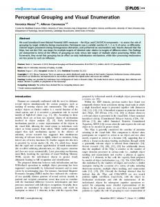
Figure 2: Illustration of the TAG framework used for training. Left: The system learns by denoising its input over iterations using several groups to distribute the representation. Each group, represented by several panels of the same color, maintains its own estimate of reconstructions z i of the input, and corresponding masks mi , which encode the parts of the input that this group is responsible for representing. These estimates are updated over iterations by the same network, that is, each group and iteration share the weights of the network and only the inputs to the network differ. In the case of images, z contains pixel-values. Right: In each iteration z i−1 and mi−1 from the previous iteration, are used to compute a likelihood term L(mi−1 ) and modeling error δz i−1 . These four quantities are fed to the parametric mapping to produce z i and mi for the next iteration. During learning, all inputs to the network are derived from the corrupted input as shown here. The unsupervised task for the network is to learn to denoise, i.e. output an estimate q(x) of the original clean input. See Section 2.1 for more details.

knowing the underlying generative model. This works as long as the network is provided with the input information and mechanisms required for an an efficient approximation of posterior inference. 2.1

Definition of the TAG mechanism

Figure 2 shows an illustration of the TAG framework. A high-level overview is that we train an iterative network to denoise corrupted inputs using backpropagation. Given an input x, we first corrupt it with noise into x ˜, which is the only version that we show to the network during training. We use Gaussian noise for the continuous case and bit-flip noise for the binary case. The output of each iteration of the network is an approximation qi (x) of the true probability p(x | x ˜), which is refined over iterations indexed by i. We mostly omit i from the equations for readability. As the cost function for training the network, we use the negative log likelihood C(x) = −

X

log q(xj ),

(1)

j

where the summation is over elements j of the input. Since this cost function does not require any class labels or intended grouping information, training can be completely unsupervised, though additional terms for supervised tasks can be added too. Group representation. Internally, the network maintains G versions of its representations, which are indexed by g. These internal representations are zg , the expected value of the input, and mg , which represents the group assignment probabilities: mg,j = q(gj ) = q(Kj = g). Each zg and mg has the same dimensionality as the input, and they are updated over iterations. Each group g makes its own prediction about the original input based on zg . In the binary case we use Q(Xj | gj ) = sigmoid(zg,j ), and in the continuous case we take zg,j to represent the mean of a Gaussian distribution. We assumed the variance of the Gaussian distribution to be constant over iterations and groups but learned it from the data. It would be easy to add a more accurate estimate of the variance. 3

The final prediction of the network is define as: X X q(xj ) = q(gj )q(xj | gj ) = mg,j q(xj | gj ). g

(2)

g

The group assignment probabilities q(gj ) = mg are forced to be non-negative and sum up to one over g: X mg,j ≥ 0, mg,j = 1. (3) g

Inputs. In contrast to a normal denoising autoencoder that receives the corrupted x ˜, we feed in estimates mig and zgi from the previous iteration and two quantities, L(mig ) and δzgi . They are functions of the estimates and the corrupted x ˜ and carry information about how the estimates could be improved. A parametric mapping then produces the new estimates mi+1 and zgi+1 . The initial g 0 0 values for mg are randomized, and zg is set to the data mean for all g. Since we are using denoising as a target objective, the network can only be allowed to take inputs through the corrupted x ˜ during learning. Therefore, we need to look at the likelihood p(˜ x | z: , g) of the corrupted input when trying to determine how the estimates could be improved. Since gj are discrete variables unlike zg,j , we treat them slightly differently: For gj it is feasible to express the complete likelihood table assuming other values constant. We denote this function by L(mg,j ) ∝ q(˜ xj | z:,j , gj ) .

(4)

Note that we normalize L(mg,j ) over g such that it sums up to one for each value of j. This amounts to providing each group information about which input element belongs to them rather than some other group. In other words, this is equivalent to likelihood ratio rather than the raw likelihood. Intuitively, the term L(mg ) describes how well each group reconstructs the individual input elements relative to the other groups. Because zg are continuous variables, their likelihood is a function over all possible values of zg , and not all of this information can be easily represented. Typically, the relevant information is found close to the current estimate zg ; therefore we use δzg , which is proportional to the gradient of the negative log likelihood. Essentially, it represents the remaining modeling error: δzg,j = mg,j (˜ xj − zg,j ) ∝

∂ [− log q(˜ xj | z:,j , gj )] . ∂zg,j

(5)

The derivation of the analogous term in the binary case is presented in Appendix A.2. Parametric mapping. The final component needed in the TAG framework is the parametric model, which does all the heavy lifting of inference. This model has a dual task: first, to denoise the estimate zg of what each group says about the input, and second, to update the group assignment probabilities mg of each input element. The information about the remaining modeling error is based on the corrupted input x ˜; thus, the parametric network has to denoise this and in effect implement posterior inference for the estimated quantities. The mapping function is the same for each group g and for each iteration. In other words, we share weights and in effect have only one function approximator that we reuse. The denoising task encourages the network to iteratively group its inputs into coherent groups that can be efficiently modeled. The trained network can be useful for a real-world denoising application, but typically, the concept is to encourage the network to learn interesting internal representations. Therefore, it is not q(x) but rather mg , zg and the internal representations of the parametric mapping that we are typically concerned with. 2.2

The Tagger: Combining TAG and Ladder Network

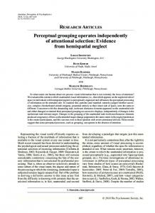
We chose the Ladder network [17] as the parametric mapping because its structure reflects the computations required for posterior inference in hierarchical latent variable models. This means that the network should be well equipped to handle the hierarchical structure one might expect to find in many domains. We call this Ladder network wrapped in the TAG framework Tagger. This is illustrated in Figure 3. 4

ygi

zig

mig L(mig )

zig

zi+1 mi+1 g g

Figure 3: An example of how Tagger would use a 3-layer-deep Ladder Network as its parametric mapping to perform its iteration i + 1. Note the optional class prediction output ygi for classification tasks. See Section 2.2 for details.

We mostly used the specifications of the Ladder network as described by Rasmus et al. [17], but there are some minor modifications we made to fit it to the TAG framework. We found that the model becomes more stable during iterations when we added a sigmoid function to the gating variable v [17, Equation 2] used in all the decoder layers with continuous outputs. None of the noise sources or denoising costs were in use (i.e., λl = 0 for all l in Eq. 3 of Ref. [17]), but Ladder’s classification cost (Cc in Ref. [17]) was added to the Tagger’s cost (Equation 1) for the semi-supervised tasks. All four inputs (zgi , mig , δzgi , and L(mig )) were concatenated and projected to a hidden representation that served as the input layer of the Ladder Network. Subsequently, the values for the next iteration ˆ in [17]) and projected linearly into zgi+1 and via softmax were simply read from the reconstruction (x to mi+1 to enforce the conditions in Equation 3. For the binary case, we used a logistic sigmoid g activation for zgi+1 .

3

Experiments and results

We explore the properties and evaluate the performance of the Tagger both in fully unsupervised settings and in semi-supervised tasks in two datasets2 . Although both datasets consist of images and grouping is intuitively image segmentation, there is no prior in the Tagger model for images. Apart from some of the baseline methods, the results generalize even if we permute all the pixels. Shapes. We use the simple Shapes dataset [19] to examine the basic properties of our system. It consists of 60,000 (train) + 10,000 (test) binary images of size 20x20. Each image contains three random chosen shapes (4, 5, or ) composed together at random positions with possible overlap. The dataset also contains the original shapes before composition, which are used only for automatic evaluation of the segmentation. Textured MNIST. We generated a two-object supervised dataset (TextureMNIST2) by sequentially stacking two textured 28x28 MNIST-digits, shifted two pixels left and up, and right and down, respectively, on top of a background texture. The textures for the digits and background are different randomly shifted samples from a bank of 20 sinusoidal textures with different frequencies and orientations. We use a 50k training set, 10k validation set, and 10k test set to report the results. The dataset is assumed to be difficult due to the heavy overlap of the objects in addition to the clutter 2

The datasets and a Theano [30] implementation of Tagger are available at http://github.com/ CuriousAI/tagger

5

Denoising cost AMI

Iter 1 0.094 0.57

Iter 2 0.068 0.75

Iter 3 0.063 0.80

Iter 4 0.063 0.81

(a) Convergence of Tagger over iterative inference

Iter 5 0.063 0.82

Tagger Reconst. Clust. [8]

AMI 0.82 0.61

(b) Method comparison

Table 1: Table (a) shows how quickly the algorithm evaluation converges over inference iterations with Shapes dataset. Table (b) compares segmentation quality to previous work on the Shapes dataset. The AMI score is defined in the range from 0 (guessing) to 1 (perfect match).

due to the textures. We also use a textured single-digit version (TextureMNIST1) without a shift to isolate the impact of texturing from multiple objects. An example from this dataset is presented in Figure 5 D. The datasets also contain labels and ground through pixels for digits for segmentation evaluation. 3.1

Training and evaluation

We train Tagger in an unsupervised manner by only showing the network the raw input example x, not ground truth masks or any class labels, using 4 groups and 3 iterations. We average the cost in Equation 1 over the iterations and use ADAM [12] for optimization. The Shapes dataset was trained for 100 epochs with a bit-flip probability of 0.2, and the TextureMNIST dataset was trained for 200 epochs with a noise standard deviation of 0.2. To understand how model size, length of the iterative inference, and the number of groups affect the modeling performance, we evaluate the trained models using two metrics. First, we use the cost in Equation 1 on the validation set and second, consistent with Greff et al. [8], we evaluate the segmentation into objects using the Adjusted Mutual Information (AMI) score [32] and ignore the background and overlap regions in the Shapes dataset. Evaluations of the AMI score and classification results in semi-supervised tasks were performed with uncorrupted input. The system has no restrictions regarding the number of groups and iterations used for training and evaluation. The results improved in terms of both denoising cost and AMI score when iterating further, so we used 5 iterations for testing. Even if the system was trained with 4 groups and 3 shapes per training example, we could test the evaluation with, for example, 2 groups and 3 shapes, or 4 groups and 4 shapes. 3.2

Unsupervised Perceptual Grouping

Table 1 shows the median performance of Tagger on the Shapes dataset over 20 seeds. Tagger is able to achieve very fast convergences, as shown in Table 1a. Through iterations, the network improves its denoising performances by grouping different objects into different groups. Comparing to Greff et al. [8], Tagger performs significantly better in terms of AMI score (see Table 1b). Figure 4 and Figure 5 qualitatively show the learned unsupervised groupings for the Shapes and textured MNIST datasets. Tagger uses its TAG mechanism slightly differently for the two datasets. For Shapes, zg represents filled-in objects and masks mg show which part of the object is actually visible. For textured MNIST, zg represents the textures and masks mg texture segments. In the case of the same digit or two identical shapes, Tagger can segment them into separate groups, and hence, it performs instance segmentation. We used 4 groups for training even though there are only 3 objects in the Shapes dataset and 3 segments in the TexturedMNIST2 dataset. The excess group is left empty by the trained system but their presence seems to speed up the learning process. The hand-picked examples A-C in Figure 4 illustrate the robustness of the system when the number of objects changes in the evaluation dataset or when evaluation is performed using fewer groups. Example E is particularly interesting; E1 shows how the normal evaluation looks like but E2 demonstrates how we can remove the topmost digit from the scene and let the system fill in digit below and the background. We do this by manually setting the corresponding group assignment probabilities mg to a large negative number just before the final softmax over groups in the last iteration. 6

i=1

i=2

i=3

i=4

C

m3

B

z3

A

m2

0. 52

z2

0. 61

m1

0. 88

z1

1. 00

m0

1. 00

z0

1. 00

1. 00

reconst.

i=0

original

reconst.

Figure 4: Results for Shapes dataset. Left column: 7 examples from the test set along with their resulting groupings in descending AMI score order and 3 hand-picked examples (A, B, and C) to demonstrate generalization. A: Testing 2-group model on 3 object data. B: Testing a 4-group model trained with 3-object data on 4 objects. C: Testing 4-group model trained with 3-object data on 2 objects. Right column: Illustration of the inference process over iterations for four color-coded groups; mg and zg .

7

i=1

i=2

i=3

i=4

0. 93

reconst.

i=0

E2

m3

Pred. : 4

E1

z3

D

m2

0. 76

Pred. : no class

z2

0. 76

m1

0. 79

Pred. : 3

z1

0. 85

m0

0. 91

Pred. : no class

z0

0. 87

Class

original

reconst.

Figure 5: Results for the TextureMNIST2 dataset. Left column: 7 examples from the test set along with their resulting groupings in descending AMI score order and 3 hand-picked examples (D, E1, E2). D: An example from the TextureMNIST1 dataset. E1-2: A hand-picked example from TextureMNIST2. E1 demonstrates typical inference, and E2 demonstrates how the system is able to estimate the input when a certain group (topmost digit 4) is removed. Right column: Illustration of the inference process over iterations for four color-coded groups; mg and zg .

8

To solve the textured two-digit MNIST task, the system has to combine texture cues with high-level shape information. The system first infers the background texture and mask which are finalized on the first iteration. Then the second iteration typically fixes the texture used for topmost digit, while subsequent iterations clarify the occluded digit and its texture. This demonstrates the need for iterative inference of the grouping. 3.3

Classification

We investigate the role of grouping for the task of classification. We evaluate the Tagger against four baseline models on the textured MNIST task. As our first baseline we use a fully connected network (FC) with ReLU activations and batch normalization after each layer. Our second baseline is a ConvNet (Conv) based on Model C from [28], which has close to state-of-the-art results on CIFAR-10. We removed dropout, added batch normalization after each layer and replaced the final pooling by a fully connected layer to improve its performance for the task. Furthermore, we compare with a fully connected Ladder [17] (FC Ladder) network. All models use a softmax output and are trained with 50,000 samples to minimize the categorical cross entropy error. In case there are two different digits in the image (most examples in the TextureMNIST2 dataset), the target is p = 0.5 for both classes. We evaluate the models based on classification errors. For the two-digit case, we score the network based on the two highest predicted classes (top 2). For Tagger, we first train the system in an unsupervised phase for 150 epochs and then add two fresh randomly initialized layers on top and continue training the entire system end to end using the sum of unsupervised and supervised cost terms for 50 epochs. Furthermore, the topmost layer has a per-group softmax activation that includes an added ’no class’ neuron for groups that do not contain any digit. The final classification is then performed by summing the softmax output over all groups for the true 10 classes and renormalizing this sum to add up to one. The final results are summarized in Table 2. As shown in this table, Tagger performs significantly better than all the fully connected baseline models on both variants, but the improvement is more pronounced for the two-digit case. This result is expected because for cases with multi-object overlap, grouping becomes more important. It, moreover, confirms the hypothesis that grouping can help classification and is particularly beneficial for complex inputs. Remarkably, Tagger, despite being fully connected, is on par with the convolutional baseline for the TexturedMNIST1 dataset and even outperforms it in the two-digit case. We hypothesize that one reason for this result is that grouping allows for the construction of efficient invariant features already in the low layers without losing information about the assignment of features to objects. Convolutional networks solve this problem to some degree by grouping features locally through the use of receptive fields. But that strategy is expensive and can break down in cases of heavy overlap. 3.4

Semi-Supervised Learning

Training TAG does not rely on labels and is therefore directly usable in a semi-supervised context. For semi-supervised learning, the Ladder [17] is arguably one of the strongest baselines with SOTA results on 1,000 MNIST and 60,000 permutation invariant MNIST classification. We follow the common practice of using 1,000 labeled samples and 49,000 unlabeled samples for training Tagger and the Ladder baselines. For completeness, we also report results of the convolutional (ConvNet) and fully-connected (FC) baselines trained fully supervised on only 1,000 samples. From the results in Table 2, it is obvious that all the fully supervised methods fail on this task with 1,000 labels. The best result of approximately 52 % error for the single-digit case is achieved by ConvNet, which still performs only at chance level for two-digit classification. The best baseline result is achieved by the FC Ladder, which reaches 30.5 % error for one digit but 68.5 % for TextureMNIST2. For both datasets, Tagger achieves by far the lowest error rates: 10.5 % and 24.9 %, respectively. Again, this difference is amplified for the two-digit case, where the Tagger with 1,000 labels even outperforms the Ladder baseline with all labels. This result matches our intuition that grouping can often segment out objects even of an unknown class and thus help select the relevant features for learning. This is particularly important in semi-supervised learning where the inability to self-classify unlabeled samples can easily mean that the network fails to learn from them at all. 9

Dataset TextureMNIST1

Method FC MLP FC Ladder FC Tagger (ours) ConvNet

Error 50k

Error 1k

31.1 ± 2.2 7.2 ± 0.1 4.0 ± 0.3 3.9 ± 0.3

89.0 ± 0.2 30.5 ± 0.5 10.5 ± 0.9 52.4 ± 5.3

Model details 2000-2000-2000 / 1000-1000 3000-2000-1000-500-250 3000-2000-1000-500-250 based on Model C [28]

FC MLP 55.2 ± 1.0 79.4 ± 0.3 2000-2000-2000 / 1000-1000 FC Ladder 41.1 ± 0.2 68.5 ± 0.2 3000-2000-1000-500-250 FC Tagger (ours) 7.9 ± 0.3 24.9 ± 1.8 3000-2000-1000-500-250 ConvNet 12.6 ± 0.4 79.1 ± 0.8 based on Model C [28] Table 2: Test-set classification errors for textured one-digit MNIST (chance level: 90 %) and top-2 error on the textured two-digit MNIST dataset (chance level: 80 %). We report mean and sample standard deviation over 5 runs. FC = Fully Connected TextureMNIST2

To put these results in context, we performed informal tests with five human subjects. The task turned out to be quite difficult and the subjects needed to have regular breaks to be able to maintain focus. The subjects improved significantly over training for a few days but there were also significant individual differences. The best performing subjects scored around 10 % error for TextureMNIST1 and 30 % error for TextureMNIST2. For the latter task, the test subject took over 30 seconds per sample.

4

Related work

Attention models have recently become very popular, and similar to perceptual grouping they help in dealing with complex structured inputs. These models are not, however, mutually exclusive and can benefit from each other. Overt attention models [26, 5] control a window (fovea) to focus on relevant parts of the inputs. Their ability to reduce the problem size by limiting the field of view can help to reduce the complexity of the target problem and thus also help segmentation. Two of their limitations are that they are mostly tailored to the visual domain and are usually only suited to objects that are roughly the same shape as the window. Inspired by what is called covert attention in cognitive science, soft attention mechanisms [24, 3, 37] use some form of top-down feedback to suppress inputs that are irrelevant for a given task. These mechanisms have been recently gaining popularity, first in machine translation [1] and then applied to many other problems such as image caption generation [36]. All of these methods re-weigh the inputs based on their relevance and could benefit from a perceptual grouping process that structures the inputs. In this way, the attention would only need to decide roughly which objects to attend to, and the precise boundaries could be refined by the grouping mechanism. Our work is primarily built upon a line of research based on the concept that the brain uses synchronization of neuronal firing to bind object representations together. This view was introduced by [33] and has inspired many early works on oscillations in neural networks (see the survey [34] for a summary). Simulating the oscillations explicitly is costly and does not mesh well with modern neural network architectures (but see [15]). Rather, complex values have been used to model oscillating activations using the phase as soft tags for synchronization [16, 18]. In our model, we use an even further abstraction that discretizes these. It is most similar to the models of Wersing et al. [35] and Greff et al. [8]. However, our work is the first to combine this with denoising autoencoders in an end-to-end trainable fashion. Another closely related line of research [21, 20] has focused on multi-causal modeling of the inputs. Many of the works in that area [14, 29, 27, 11] build upon Restricted Boltzmann Machines. Each input is modeled as a mixture model with a separate latent variable for each object. Because exact inference is intractable, these models approximate the posterior with some form of expectation maximization [4] or sampling procedure. Our assumptions are very similar to these approaches, but we allow the model to learn the amortized inference directly (more in line with Goodfellow et al. [7]). Since recurrent neural networks (RNNs) are general purpose computers, they can in principle implement arbitrary computable types of temporary variable binding [23, 24] and unsupervised 10

segmentation [22] and internal [24] and external attention [26]. For example, an RNN with fast weights [24] can rapidly associate or bind the patterns to which the RNN currently attends. Similar approaches even allow for metalearning [25], that is, learning a learning algorithm. Hochreiter et al. [10], for example, learned fast online learning algorithms for the class of all quadratic functions of two variables. Unsupervised segmentation could therefore in principle be learned by any RNN as a by-product of data compression or any other given task. That does not, however, imply that every RNN will, through learning, easily discover and implement this tool. From that perspective, TAG can be seen as a way of helping an RNN to quickly learn and efficiently implement a grouping mechanism. We believe this special case of computation to be important enough for many real-world tasks to justify this added complexity.

5 5.1

Discussion Task-dependence of grouping

The “correct” grouping is often dynamic, ambiguous and task dependent. For example, when driving along a road, it is useful to group all the buildings together. To find a specific house, however, it is important to separate the buildings, and to enter one, they need to be subdivided even further. Rather than treating segmentation as a separate task, we provided a mechanism for grouping as a tool for our system. This provides the possibility of learning how to best group its inputs depending on the task. 5.2

Future Work

So far we’ve assumed the groups to represent independent objects or events. However, this assumption is unrealistic in many cases. Assuming only conditional independence would be considerably more reasonable, and could be implemented by allowing all groups to share the same top-layer of their Ladder network. The TAG framework assumes just one level of (global) groups, which does not reflect the hierarchical structure of the world. Therefore, another important future extension is to rather use a hierarchy of local groupings, by using our model as a component of a bigger system. This could be achieved by collapsing the groups of a Tagger network by summing them together at some hidden layer. That way this abstract representation could serve as input for another tagger with new groupings at this higher level. We hypothesize that a hierarchical Tagger could also represent relations between objects, because they are simply the couplings that remain from the assumption of independent objects. Movement is a strong segmentation cue and simple temporal extensions of TAG could be to the connect higher layers forward in time, not just via the inputs. Iteration would then occur in time alongside the changing inputs. We believe that these extensions will make it possible to scale the approach to video.

6

Conclusion

In this paper, we have argued that the ability to group input elements and internal representations is a powerful tool that can improve a system’s ability to handle complex multi-object inputs. We have introduced the TAG framework, which enables a network to directly learn the grouping and the corresponding amortized iterative inference in a unsupervised manner. The resulting iterative inference is very efficient and converges within 5 iterations. We have demonstrated the benefits of this mechanism for a heavily cluttered classification task, in which our fully connected Tagger even significantly outperformed a state-of-the-art convolutional network. More impressively, we have shown that our mechanism can greatly improve semi-supervised learning, exceeding conventional Ladder networks by a large margin. Our method takes minimal assumptions about the data and can be applied to any modality. With TAG, we have barely scratched the surface of a comprehensive integrated grouping mechanism, but we already see significant advantages. We believe grouping to be crucial to human perception and are convinced that it will help to scale neural networks to even more complex tasks in the future . 11

Acknowledgments The authors wish to acknowledge useful discussions with Theofanis Karaletsos, Jaakko Särelä, Tapani Raiko and Søren Kaae Sønderby. And further acknowledge the rest of the Curious AI Company team for computational infrastructure, human testing and other support. This research was supported by the EU project “INPUT” (H2020- ICT-2015 grant no. 687795).

References [1] Bahdanau, D., Cho, K., and Bengio, Y. Neural machine translation by jointly learning to align and translate. arXiv preprint arXiv:1409.0473, 2014. [2] Bengio, Y., Thibodeau-Laufer, E., Alain, G., and Yosinski, J. Deep generative stochastic networks trainable by backprop. JMLR, 2014. [3] Deco, G. Biased competition mechanisms for visual attention in a multimodular neurodynamical system. In Emergent neural computational architectures based on neuroscience, pp. 114–126. Springer, 2001. [4] Dempster, A. P., Laird, N. M., and Rubin, D. B. Maximum likelihood from incomplete data via the EM algorithm. Journal of the royal statistical society., pp. 1–38, 1977. [5] Eslami, S. M., Heess, N., Weber, T., Tassa, Y., Kavukcuoglu, Y., and Hinton, G. E. Attend, Infer, Repeat: Fast Scene Understanding with Generative Models. preprint arXiv:1603.08575, 2016. [6] Gallinari, P., LeCun, Y., Thiria, S., and Fogelman-Soulie, F. Mémoires associatives distribuées: une comparaison (distributed associative memories: a comparison). In Cesta-Afcet, 1987. [7] Goodfellow, I. J., Bulatov, Y., Ibarz, J., Arnoud, S., and Shet, V. Multi-digit number recognition from street view imagery using deep convolutional neural networks. arXiv preprint arXiv:1312.6082, 2013. [8] Greff, K., Srivastava, R. K., and Schmidhuber, J. Binding via Reconstruction Clustering. arXiv:1511.06418 [cs], November 2015. [9] Gregor, K. and LeCun, Y. Learning fast approximations of sparse coding. In Proceedings of the 27th International Conference on Machine Learning (ICML-10), pp. 399–406, 2010. [10] Hochreiter, S., Younger, A. S., and Conwell, P. R. Learning to learn using gradient descent. In Proc. International Conference on Artificial Neural Networks, pp. 87–94. Springer, 2001. [11] Huang, J. and Murphy, K. Efficient inference in occlusion-aware generative models of images. arXiv preprint arXiv:1511.06362, 2015. [12] Kingma, D. and Ba, J. Adam: A method for stochastic optimization. ICLR, 2015. [13] Le Cun, Y. Modèles connexionnistes de l’apprentissage. PhD thesis, Paris 6, 1987. [14] Le Roux, N., Heess, N., Shotton, J., and Winn, J. Learning a generative model of images by factoring appearance and shape. Neural Computation, 23(3):593–650, 2011. [15] Meier, M., Haschke, R., and Ritter, H. J. Perceptual grouping through competition in coupled oscillator networks. Neurocomputing, 141:76–83, 2014. [16] Rao, R. A., Cecchi, G., Peck, C. C., and Kozloski, J. R. Unsupervised segmentation with dynamical units. Neural Networks, IEEE Transactions on, 19(1):168–182, 2008. [17] Rasmus, A., Berglund, M., Honkala, M., Valpola, H., and Raiko, T. Semi-Supervised Learning with Ladder Networks. In NIPS, pp. 3532–3540, 2015. [18] Reichert, D. P. and Serre, T. Neuronal Synchrony in Complex-Valued Deep Networks. arXiv:1312.6115 [cs, q-bio, stat], December 2013. 12

[19] Reichert, D. P., Series, P, and Storkey, A. J. A hierarchical generative model of recurrent object-based attention in the visual cortex. In ICANN, pp. 18–25. Springer, 2011. [20] Ross, D. A. and Zemel, R. S. Learning parts-based representations of data. The Journal of Machine Learning Research, 7:2369–2397, 2006. [21] Saund, E. A multiple cause mixture model for unsupervised learning. Neural Computation, 7 (1):51–71, 1995. [22] Schmidhuber, J. Learning complex, extended sequences using the principle of history compression. Neural Computation, 4(2):234–242, 1992. [23] Schmidhuber, J. Learning to control fast-weight memories: An alternative to dynamic recurrent networks. Neural Computation, 4(1):131–139, 1992. [24] Schmidhuber, J. Reducing the Ratio Between Learning Complexity and Number of Time Varying Variables in Fully Recurrent Nets. In ICANN’93, pp. 460–463. Springer, 1993. [25] Schmidhuber, J. A ‘Self-Referential’Weight Matrix. In ICANN’93, pp. 446–450. Springer, 1993. [26] Schmidhuber, J. and Huber, R. Learning to generate artificial fovea trajectories for target detection. International Journal of Neural Systems, 2(01n02):125–134, 1991. [27] Sohn, K., Zhou, G., Lee, C., and Lee, H. Learning and selecting features jointly with point-wise gated ${$b$}$ oltzmann machines. In Proceedings of The 30th International Conference on Machine Learning, pp. 217–225, 2013. [28] Springenberg, J. T., Dosovitskiy, A., Brox, T., and Riedmiller, M. Striving for simplicity: The all convolutional net. arXiv preprint arXiv:1412.6806, 2014. [29] Tang, Y., Salakhutdinov, R., and Hinton, G. Robust boltzmann machines for recognition and denoising. In Computer Vision and Pattern Recognition (CVPR), 2012 IEEE Conference on, pp. 2264–2271. IEEE, 2012. [30] The Theano Development Team. Theano: A Python framework for fast computation of mathematical expressions. arXiv:1605.02688 [cs], May 2016. [31] Vincent, P., Larochelle, H., Bengio, Y., and Manzagol, P. A. Extracting and composing robust features with denoising autoencoders. In ICML, pp. 1096–1103. ACM, 2008. [32] Vinh, N. X., Epps, J., and Bailey, J. Information theoretic measures for clusterings comparison: Variants, properties, normalization and correction for chance. The Journal of Machine Learning Research, 11:2837–2854, 2010. [33] von der Malsburg, C. The Correlation Theory of Brain Function. 1981. [34] Von Der Malsburg, C. Binding in models of perception and brain function. Current opinion in neurobiology, 5(4):520–526, 1995. [35] Wersing, H., Steil, J. J., and Ritter, H. A competitive-layer model for feature binding and sensory segmentation. Neural Computation, 13(2):357–387, 2001. [36] Xu, K., Ba, J., Kiros, R., Courville, A., Salakhutdinov, R., Zemel, R., and Bengio, Y. Show, attend and tell: Neural image caption generation with visual attention. arXiv preprint arXiv:1502.03044, 2015. [37] Yli-Krekola, A., Särelä, J., and Valpola, H. Selective attention improves learning. In Artificial Neural Networks–ICANN 2009, pp. 285–294. Springer, 2009.

13

A A.1

Supplementary Material Notation

x input vector with elements xj x ˜ corrupted input p(x | x ˜) posterior of the data given the corrupted data q(x) learnt approximation of p(x | x ˜) zg the predicted mean of input for each group g. Has the same dimensions as the input q(xj | gj ) Shorthand for q(xj | Kj = g), that is the probability which group g assigns to the input mg probabilities for the group assignment. Has the same dimensions as the input. i iteration index j input element index g group index, takes values between 1 and G δzg prediction error for group g L(mg ) normalized likelihood, expresses how likely it looks for each individual pixel to be produced by group g A.2

Derivation of δz in the Binary Case

As explained in Sec. 2.1, δz carries information about the remaining prediction error. Since during learning, we are only allowed to input information about the corrupted x ˜ but not the original clean x, we cannot use the derivative −∂C/∂zg,j . Rather, we define X X C˜ = P (˜ xj | zg,j )mg,j ) . − log( j

g

˜ and use −∂ C/∂z g,j . In the continuous case we model the input as a Gaussian variable with mean z so it makes sense to simply use δzg,j = mg,j (˜ xj − zg,j ) ∝ −∂ C˜d (x)/zg,j . Note that since the network will multiply its inputs with weights, we can always omit any constant multipliers. In the following, we will drop the index j, the input element index, because we can work on each input element separately. Let us denote the corruption bit-flip probability by β and define ξg := EP (x|zg ) {x} = (1 − 2β)zg + β . We then have P (˜ x | zg ) = x ˜ξg + (1 − x ˜)(1 − ξg ) ∂ C˜ 1 = −P ∂P (˜ x|zg )mg ∂zg x | zg0 )mg0 g 0 P (˜ ∂zg =−

(˜ x(1 − 2β) − (1 − x ˜)(1 − 2β))mg P P (˜ x | z g 0 )mg 0 g0

(˜ x(1 − 2β) − (1 − x ˜)(1 − 2β))mg =− P xξg + (1 − x ˜)(1 − ξg ))sg0 g 0 (˜ which simplifies for x ˜ = 1 as (1 − 2β)mg mg =− P ≈ −P 0 0 g 0 ξg mg g 0 ξg mg 14

and for x ˜ = 0 as =

(1 − 2β)mg m mg P P g ≈ = −P 0 ξ 1 − g0 ξg mg0 1 − g0 ξg mg0 g 0 g mg − 1

Putting it back together: mg ∂ C˜ = −P 0 ∂zg ˜ g 0 ξg mg − 1 + x

15