representations of this model include time series such as Auto-regressive ...... the HVAC system is divided into two parts; building and AHU model and indoor ...... pleasantness under varying atmospheric conditionsâ Trans american society of ...
TAKAGI-SUGENO FUZZY MODELLING AND ADAPTIVE CONTROL OF INDOOR THERMAL COMFORT IN HVAC SYSTEMS USING PREDICTED MEAN VOTE INDEX
RAAD Z. HOMOD
COLLEGE OF GRADUATE STUDIES UNIVERSITI TENAGA NASIONAL
2012
TAKAGI-SUGENO FUZZY MODELLING AND ADAPTIVE CONTROL OF INDOOR THERMAL COMFORT IN HVAC SYSTEMS USING PREDICTED MEAN VOTE INDEX
BY
RAAD Z. HOMOD
A Thesis Submitted in Fulfillment of the Requirement for the Degree of Doctor of Philosophy,
College of Graduate Studies Universiti Tenaga Nasional
FEBRUARY 2012
I dedicated this thesis to my beloved mother, father, wife and children
ABSTRACT
The purpose of Heating, Ventilating and Air Conditioning (HVAC) system is to provide and maintain a desired indoor thermal comfort. Modelling process of HVAC systems leads to inherent nonlinearity of the large scale system including pure lag time, big thermal inertia, uncertain disturbance factors and constraints which lead to inability to control this system. There are many modeling approaches available to control HVAC system and the techniques have become quite mature. But there is no combined model developed for the comprehensive HVAC system. This study addresses this issue by proposing a hybrid model combing building structure with the equipments of HVAC system in one model. The hybrid identification is built with physical and empirical functions of thermal inertia quantity. The empirical Residential Load Factor (RLF), which is modelled by Residential Heat Balance (RHB), is required to calculate a building cooling/heating load. The model parameters can be calculated differently from room to room and are appropriate for variable air volume (VAV) factor. In this research work, a pre-cooling coil is added to humidify the incoming air, which controls the humidity more efficiently inside conditioned space. To evaluate indoor thermal comfort situations, Predicted Mean Vote (PMV) and Predicted Percentage of Dissatisfaction (PPD) indicators were used. This modelling part is represented as a fuzzy PMV/PPD model which is regarded as a white-box model. This modelling is achieved using a Takagi-Sugeno (TS) fuzzy model and tuned by Gauss-Newton Method for Nonlinear Regression (GNMNR) algorithm. To control such sophisticated HVAC system, this study proposes a new online tuned Takagi-Sugeno Fuzzy Forward (TSFF). The identification of study for HVAC system and PMV models by both hybrid method and converting a TakagiSugeno fuzzy inference system (TSFIS) model into memory layers parameters (TS model) is computationally faster and efficient than traditional methods. Furthermore the hybrid modelling and converting TSFIS to TS model are suitable techniques to represent their nonlinearities. Both models have been successfully validated by both theoretical and numerical methods. The TS controller model is based on converting TSFIS to TS, which is well-suited for mathematical analysis. Furthermore, the outputs routine of the classical TSFIS model requires numerical and logical operation tasks and this consumes time. Additionally TS controller model works well with optimization and adaptive techniques based on GNMNR and gradient methods. These two algorithms have guaranteed convergence of the optimized inputs to the online control target. The comparison testing results demonstrate that the proposed TSFF control strategy gives superior performance, adaptation, robustness and high precision compared to the traditional controllers.
i
ACKNOWLEDGMENT
First and foremost, I am very faithful to Allah for giving me the strength, good health and allowing me to complete this thesis. I would like also to express my appreciation to many people who helped significantly in preparing this thesis. First, I would like to sincerely thank my supervisor Dr. Khairul Salleh Mohamed Sahari for his efforts and guidance during all stage of this thesis. My thanks are also to co-supervisors Dr. Haider A.F. Almurib and Dr. Farrukh Hafiz Nagi for their help and advice on the subject area of artificial intelligent controls and their application. And then I would like to thank my friends inside and outside of the faculty. Finally, I would like to express my great appreciation for my father, mother and brothers for their patience and encouragement. Last but not least, I wish to give my sincere gratitude and deepest love to my wife and children for their continuous love and support, which enabled the completion of my thesis work.
ii
DECLARATION
I hereby declare that this thesis, submitted to Universiti Tenaga Nasional as fulfillment of the requirements for the degree of Doctor of Philosophy has not been submitted as an exercise for a similar degree at any other university. I also certify that the work described here is entirely my own except for excerpts and summaries whose sources are appropriately cited in the references.
This thesis may be made available within university the library and may be photocopied or loaned to other libraries for the purpose of consultation.
FEBRUARY 2012
Raad Z. Homod
iii
TABLE OF CONTENTS
Page ABSTRACT ............................................................................................................ I ACKNOWLEDGMENT ...................................................................................... II DECLARATION .................................................................................................. III TABLE OF CONTENTS .................................................................................... IV LIST OF FIGURES ............................................................................................. IX LIST OF TABLES .............................................................................................. XIII LIST OF NOMENCLATURE, SYMBOLS AND ACRONYMS .................... XIV 1- LIST OF ABBREVIATIONS .................................................................................. XIV 2- LIST OF SYMBOLS............................................................................................. XV 3- SUBSCRIPTS ..................................................................................................... XVIII CHAPTER 1 INTRODUCTION ..........................................................................1 1.0 INTRODUCTION .................................................................................................1 1.1 THE HVAC SYSTEMS MODEL ..........................................................................1 1.1.1 Mathematical model of HVAC system...................................................3 1.1.2 Black box model of HVAC system ........................................................4 1.1.3 Gray-box models of HVAC system ........................................................4 1.2 THE HVAC SYSTEM CONTROL .........................................................................5 1.3 THE HVAC SYSTEM SIMULATION ....................................................................6 1.4 PROBLEM STATEMENT ......................................................................................8 1.5 RESEARCH OBJECTIVES ....................................................................................9 1.6 SCOPE OF STUDY ..............................................................................................10 1.7 THESIS OUTLINE ..............................................................................................11 1.8 SUMMARY .......................................................................................................11 CHAPTER 2 HVAC SYSTEM LITERATURE REVIEW .............................13 2.0 INTRODUCTION ................................................................................................13 iv
2.1 BUILDING AND AHU MODEL ...........................................................................15 2.1.1 The evolution of modelling HVAC system ...........................................15 2.1.2 Mathematical model ..............................................................................16 2.1.3 Black box model ....................................................................................18 2.1.4 Gray box model .....................................................................................20 2.2 INDOOR THERMAL COMFORT MODEL ...............................................................22 2.2.1 The evolution of thermal comfort ..........................................................22 2.2.2 The predicted mean vote (PMV) index .................................................23 2.2.3 PMV models ..........................................................................................25 2.3 HVAC SYSTEM CONTROL ...............................................................................27 2.3.1 The evolution of HVAC system control ................................................28 2.3.2 PID control for HVAC system ..............................................................29 2.3.3 Fuzzy logic control for HVAC system ..................................................32 2.4 THE SHORTCOMING IN PREVIOUS WORKS AND ALTERNATIVES ......................35 2.4.1 Modelling of building and AHU............................................................35 2.4.2 Modelling of indoor thermal comfort ....................................................37 2.4.3 The control algorithms...........................................................................38 2.5 SUMMARY .......................................................................................................40 CHAPTER 3 MODELLING OF HVAC SYSTEM ............................................42 3.0 INTRODUCTION ................................................................................................42 3.1 MODIFICATION OF HVAC SYSTEM ..................................................................43 3.2 BUILDING AND AHU MODEL ...........................................................................43 3.2.1 System description .................................................................................46 3.2.2 Modeling approach ................................................................................47 i. Thermal transmittance .................................................................................48 ii. Moisture transmittance ...............................................................................48 iii. Model linearization....................................................................................49 3.2.3 Model development ...............................................................................50 i. Pre-cooling coil............................................................................................50 ii. Mixing air chamber ....................................................................................53 iii. Main cooling coil.......................................................................................55 iv. Building structure ......................................................................................57 a) b) c)
Opaque surfaces ................................................................................... 57 Transparent fenestration surfaces........................................................ 60 Slab floors ............................................................................................ 64 v
v. Conditioned space .......................................................................................66 3.3 INDOOR THERMAL COMFORT MODEL ...............................................................70 3.3.1 General idea ...........................................................................................72 3.3.2 Data pre-processing ...............................................................................74 3.3.3 Identification of TS model .....................................................................75 3.3.4 Tuning of TS model ...............................................................................77 3.4 SUMMARY .......................................................................................................79 CHAPTER 4 CONTROL OF HVAC SYSTEM .................................................81 4.0 INTRODUCTION ................................................................................................81 4.1 DESIGN AND STRUCTURE OF TSFF CONTROLLER.............................................82 4.2 TS CONTROL MODEL ........................................................................................84 4.2.1 The related factors for input/output data sets ........................................84 4.2.2 General idea for clustering outputs ........................................................85 4.2.3 Identification of TS model .....................................................................87 4.2.4 Offline learning of TS model.................................................................89 4.3 ONLINE TUNING PARAMETERS .........................................................................91 4.4 SUMMARY .......................................................................................................94 CHAPTER 5 SIMULATION OF HVAC MODEL AND CONTROL...........95 5.0 INTRODUCTION ................................................................................................95 5.1 SIMULATION ENVIRONMENT ............................................................................96 5.2 SIMULATION OF THE BUILDING AND AHU MODEL ...........................................99 5.2.1 Subsystem block diagram .....................................................................100 5.2.2 Overall block diagram model ...............................................................101 5.2.3 HVAC system Model validation ..........................................................105 5.3 SIMULATION OF THE INDOOR THERMAL COMFORT MODEL ..............................106 5.3.1 Parameters and weight layers identification procedures ......................107 5.3.2 TS Model validation .............................................................................108 5.3.3 Application to combined PMV with building Model ...........................109 5.4 SIMULATION OF THE TSFF CONTROL..............................................................112 5.4.1 TS control model layers identification procedures ...............................113 5.4.2 TS control model validation .................................................................113 5.4.3 Online tuning parameters and weight ...................................................114 5.5 SIMULATION OF THE ENERGY SAVING AND MODEL DECOUPLING ....................115 5.5.1 Energy saving calculation .....................................................................116
vi
5.5.2 The model decoupling ..........................................................................119 5.6 SUMMARY ......................................................................................................122 CHAPTER 6 ANALYSIS OF RESULTS .........................................................124 6.0 INTRODUCTION ...............................................................................................124 6.1 BUILDING AND AHU MODEL ..........................................................................125 6.1.1 Open loop response...............................................................................125 6.1.2 Psychrometric process line analyses .....................................................126 6.1.3 Validation of the hybrid modeling method ...........................................127 6.1.4 Case study: evaluation of hybrid ventilation ........................................128 i. Ventilation at daytime ................................................................................130 ii. Ventilation at night ...................................................................................132 iii. Psychrometric process line analyses .........................................................133 iv. The PMV comparison ...............................................................................135 6.2 INDOOR THERMAL COMFORT MODEL ..............................................................138 6.2.1 Defining the range of comfort temperature ..........................................139 6.2.2 Comparing thermal sensation comfort with temperature .....................141 6.3 TSFF CONTROL ..............................................................................................143 6.3.1 Nominal operation conditions ..............................................................144 6.3.2 Validating robustness and disturbance rejection ..................................148 6.3.3 The sensitivity of noise and sensor deterioration .................................149 6.4 SUMMARIZED PERFORMANCE RESULTS ...........................................................153 6.5 ENERGY SAVING AND MODEL DECOUPLING ....................................................157 6.5.1 Model decoupling .................................................................................158 6.5.2 Energy saving .......................................................................................159 6.6 SUMMARY ......................................................................................................163 CHAPTER 7 CONCLUSIONS AND RACOMMENDATION OF FUTURE WORKS .................................................................................................................165 7.0 INTRODUCTION ...............................................................................................165 7.1 CONCLUSION ..................................................................................................166 7.1.1 Modelling of building and AHU...........................................................166 7.1.2 The indoor thermal comfort model .......................................................167 7.1.3 TSFF control algorithm ........................................................................168 7.2 RECOMMENDATION FOR FUTURE WORKS ........................................................170 7.2.1 Modelling of building and AHU...........................................................170
vii
7.2.2 The indoor thermal comfort model .......................................................170 7.2.3 TSFF control algorithm ........................................................................171 LIST OF REFERENCES .....................................................................................172 RELATED PUBLICATIONS ..............................................................................186 APPENDICIES......................................................................................................187 APPENDIX A: DERIVING PRE-COOLING COIL TRANSFER FUNCTION .......................187 APPENDIX B: DERIVING MIXING AIR CHAMBER TRANSFER FUNCTION..................191 APPENDIX C: DERIVING MAIN COOLING COIL TRANSFER FUNCTION .....................193 APPENDIX D: DERIVING CONDITION SPACE TRANSFER FUNCTION ........................198 APPENDIX E: THE INPUT FACTORS FOR THE BUILDING AND AHU MODEL.............203 APPENDIX F: DERIVING THE MODEL TRANSFER FUNCTION ...................................213 APPENDIX G: CONVERT THE MODEL TRANSFER FUNCTION TO EXPLICIT ...............217 APPENDIX H: THE LAYERS PARAMETERS AND WEIGHT ARE CALCULATED BY MATLAB M-FILE. ..................................................................................................227
viii
LIST OF FIGURES
Page Figure 1.1 Illustrate model staircase boxes with complexity and SNR .........2 Figure 1.2 The main fields of the HVAC system .........................................10 Figure 2.1 The main framework of the thesis ...............................................14 Figure 3.1 Flowchart for the design of HVAC systems ...............................44 Figure 3.2 Representation of subsystem using control volume concept for prototypical buildings with HVAC system ...................................................47 Figure 3.3 Thermal and moisture variation through pre-heat exchanger .....50 Figure 3.4 Thermal and moisture variation through air mixing chamber .....53 Figure 3.5 Heat transfer by face temperature difference ..............................59 Figure 3.6 Heat transfer through fenestration and windows .........................62 Figure 3.7 Heat and humidity flow in/out of conditioned space ..................68 Figure 3.8 Basis and premise membership functions with relation to cluster centers ...........................................................................................................73 Figure 3.9 Tuning schedule of GNMNR for the TS model ..........................74 Figure 3.10 Parameter values of a with respect to 𝑥1 and , , 𝑥2 ...................76 Figure 3.11 The TS model structure .............................................................77 Figure 4.1 Control structure of TSFF ...........................................................84 Figure 4.2 Basis and premise membership functions in relation to main cooling coil clustering data ...........................................................................86 Figure 4.3 The TS model structure ...............................................................88 Figure 4.4 Offline learning schedule of GNMNR for the TS model ............89 Figure 5.1 The geometry of the building chosen to get model parameters .100 Figure 5.2 Subsystems model block diagram ..............................................101 Figure 5.3 Simulation model for subsystem buildings and AHU ................102 Figure 5.4 HVAC system model block diagram..........................................103
ix
Figure 5.5 Indoor temperature response to outdoor temperature variation .106 Figure 5.6 Indoor relative humidity response to outdoor humidity ratio variation .......................................................................................................106 Figure 5.7 Compared PPD performance with TS and Fanger’s model .......108 Figure 5.8 Comparison of absolute error for TS and Fanger’s model .........109 Figure 5.9 The TS model response ..............................................................110 Figure 5.10 Schematic diagram of condition space reference control .........112 Figure 5.11 Comparison of chilled water flow rate between TS model and calculated result with absolute error ............................................................114 Figure 5.12 Simulation diagram for TSFF online tuning ............................115 Figure 5.13 Matlab block diagram for three systems simulations. ..............121 Figure 6.1 HVAC plant open loop response for indoor temperature and humidity ratio ...............................................................................................126 Figure 6.2 HVAC plant open loop response for indoor temperature and relative humidity ..........................................................................................126 Figure 6.3 Indoor thermodynamic properties transient response for whole building and HVAC plant ............................................................................127 Figure 6.4 Complete HVAC cycle and transient model response ...............128 Figure 6.5 Indoor temperature and humidity ratio response to real outdoor variation .......................................................................................................129 Figure 6.6 Indoor temperature and humidity ratio response to natural and mechanical ventilation of daytime ...............................................................131 Figure 6.7 Indoor temperature and relative humidity response to natural and mechanical ventilation of daytime ...............................................................132 Figure 6.8 Indoor temperature and humidity ratio response to natural ventilation at night .......................................................................................133 Figure 6.9 Indoor temperature and relative humidity response to natural ventilation at night .......................................................................................134 Figure 6.10 The ideal and real process line for night and day natural ventilation ....................................................................................................135 Figure 6.11 Indoor temperature and PMV comparison results between the two types of ventilation.......................................................................................136 Figure 6.12 The optimization result for the indoor temperature and PMV .137
x
Figure 6.13 The PPD as a function of the operative temperature for a typical summer and winter situation. .......................................................................140 Figure 6.14 The difference between the temperature and PPD by the response of the open loop system of the TS model. ...................................................141 Figure 6.15 Cycle path indoor temperature within 24 hours compared with PMV .............................................................................................................142 Figure 6.16 The effect of relative humidity on the PPD ..............................143 Figure 6.17 Comparison of the control performances of the HVAC system process with TSFF, normal Sugeno and hybrid PID-Cascade controllers ..146 Figure 6.18 Comparison of the indoor temperature behavior for TSFF, normal Sugeno and hybrid PID-Cascade controllers ...............................................147 Figure 6.19 Comparison of the indoor relative humidity behavior for TSFF, normal Sugeno and hybrid PID-Cascade controllers ...................................147 Figure 6.20 Comparison of the control signal variation for the main cooling coil chilled water valve for TSFF, normal Sugeno and hybrid PID-Cascade controllers ....................................................................................................148 Figure 6.21 Comparison of the control performances of the HVAC system process for the robustness and disturbance rejection ...................................149 Figure 6.22 Comparison of the indoor temperature behavior of the HVAC system process for the robustness and disturbance rejection .......................150 Figure 6.23 Comparison of the output control signal of the HVAC system process for the robustness and disturbance rejection ...................................150 Figure 6.24 Comparison of the control performances of the HVAC system process due to applied noise and sensor deterioration .................................152 Figure 6.25 Comparison between three temperature curves of the HVAC system process due to applied noise and sensor deterioration .....................152 Figure 6.26 Comparison of the output control signal of the HVAC system process due to applied noise and sensor deterioration .................................153 Figure 6.27 PMV Comparison results between the three different system designs .........................................................................................................159 Figure 6.28 Indoor temperature comparison results between the three different system designs .............................................................................................160 Figure 6.29 Indoor relative humidity comparison results between the three different system designs...............................................................................160 Figure 6.30 Controllers’ signal comparison results between the three different system designs .............................................................................................160
xi
Figure 6.31 Comparison results of the consumed energy by the cooling coil load between the three different system designs .........................................161 Figure 6.32 Comparison results of the power consumption between the three different system designs...............................................................................162
xii
LIST OF TABLES
Page Table 3.1 Input parameters range and increments ........................................74 Table 5.1 Material properties of model building construction .....................99 Table 6.1 Performance indices comparison results for three types ventilation strategies ......................................................................................................137 Table 6.2 ASHRAE Standard recommendations [132]. ..............................140 Table 6.3 Performance indices results for hyprid and TS model.................154 Table 6.4 Performance indices comparison results of TSFF, hybrid PID and fuzzy fixed for controlling indoor PMV in nominal state of operation .......155 Table 6.5 Performance indices comparison results of TSFF, hybrid PID and fuzzy fixed for controlling indoor PMV under disturbance ........................155 Table 6.6 Performance indices comparison results of TSFF, hybrid PID and fuzzy fixed for controlling indoor PMV under noise and sensor deterioration conditions .....................................................................................................156
xiii
LIST OF NOMENCLATURE, SYMBOLS AND ACRONYMS
1- List of Abbreviations AHU AI ANN ARMA
Air Handling Unit Artificial Intelligent Artificial Neural Network AutoRegressive Moving Average
ARMAX
AutoRegressive Moving Average with eXogenous input
ARX
Auto-Regressive model structure with eXogenous inputs
ASHRAE BJ
American Society of Heating, Refrigerating, and Airconditioning Engineers Box–Jenkins
CAV
Constant Air Volume
COG
Centre Of Gravity
DDC
Direct Digital Control
ET
Effective Temperature
FIS
Fuzzy Inference System
FLC
Fuzzy Logic Control
FTC
Fault Tolerant Control
GA
Genetic Algorithm
GNMNR HVAC
Gauss-Newton Method for Nonlinear Regression Heating, Ventilation, and Air Conditioning
IMC
Internal Model Control
LPC
Linear Predictive Control
LQR
Linear Quadratic Regulator
MIMO
Multi-Input Multi-Output
MPC
Model Predictive Control
NNARX OpT
Neural Network based nonlinear AutoRegressive model with eXternal inputs Operative Temperature
xiv
PID
proportional, integral and derivative
PMV
Predicted Mean Vote
PPD
Predicted Percentage of Dissatisfaction
RELS
Recursive Extended Least Squares
RLF
Residential Load Factor
SISO
Single-Input Single-Output
SNR
Signal-to-Noise Ratio
TAR
Thermal Acceptance Ratio
TSFF
Takagi-Sugeno Fuzzy Forward
TSFIS
Takagi-Sugeno Fuzzy Inference System
VAV
Variable Air Volume
VWV
Variable Water Volume
2- List of Symbols A 𝐴𝑓𝑒𝑛 𝐴𝑒𝑠 , 𝐴𝑢𝑙 𝐴𝑖 𝐴𝐿 , 𝐴𝐿,𝑓𝑙𝑢𝑒
surface area, m2 fenestration area (including frame), 𝑚2 building exposed surface area, 𝑚2 and unit leakage area, 𝑐𝑚2 /𝑐𝑚2 the set of linguistic terms Building and flue effective leakage area, 𝑐𝑚2
𝐴𝑠𝑙𝑏
area of slab floor,( 𝑚2 )
Aw
net surface area, 𝑚2
𝑎𝑖 and 𝑏𝑖
fuzzy parameters function
C
heat capacitance, 𝐽/℃
DR
cooling daily range, K
𝑑𝐸𝑠 𝑑𝑡 ∑𝑖 𝐸̇𝑖𝑛
The rate of change in the total storage energy of the system, 𝐽/𝑠
∑𝑖 𝐸̇𝑜𝑢𝑡
Total energy leaving the system, 𝐽/𝑠
L
Total energy entering the system, 𝐽/𝑠 length
𝑀𝑚 , 𝑀𝑎𝐻𝑒 , 𝑀𝐻𝑒 , 𝑀𝑤𝑙
mass of air in mixing box, in heat exchanger, heat exchanger, and wall, 𝑘𝑔
𝑐𝑝𝑎 , 𝑐𝑝𝐻𝑒 , 𝑐𝑝𝑤 , 𝑐𝑝𝑤𝑙
specific heat of moist air, heat exchanger, water and wall, 𝐽/𝑘𝑔. ℃
xv
𝑚̇𝑜,𝑡 , 𝑚̇𝑟,𝑡 , 𝑚̇𝑚,𝑡 𝑀𝑚 𝑐𝑝𝑎 𝑇𝑚,𝑡 , 𝑇𝑜,𝑡 , 𝑇𝑜𝑠,𝑡 , 𝑇𝑟,𝑡 , 𝑇𝑠,𝑡 𝑇𝑤𝑙,𝑡 , 𝑇ℎ,𝑡 , 𝑇𝑤𝑜 , 𝑇𝑤𝑖𝑛
mass flow rate of ventilation, return, mixing air at time t, 𝑘𝑔/𝑠 heat capacitance of air for mixing air chamber, 𝐽/℃ Mixing, outside, outside supply, return and supply air stream temperature at time t, ℃ Wall, Heat exchanger and chilled water out in temperature at time t, ℃
Twlou,t , TWlin ,t , 𝑇𝑔𝑖𝑛 , 𝑇𝑔𝑜𝑢
Wall and glass windows inside and outside temperature at time t, ℃
𝜔𝑠 , 𝜔𝑚 , 𝜔𝑜 , 𝜔𝑜𝑠 , 𝜔𝑟
Humidity ratio of supply, mixing, outside, outside supply and return air stream, 𝐾𝑔𝑤 ⁄𝐾𝑔𝑑𝑎
ℎ𝑓𝑔
Water latent heat of vaporization, 𝐽/𝑘𝑔
ℎ𝑖 , ℎ𝑜
Internal/external heat transfer coefficient, 𝑊/(𝑚2 . 𝐾)
𝑄̇𝑜𝑝𝑞 , 𝑄̇𝑠𝑙𝑎𝑏
opaque surface and slab cooling load, W
CF
surface cooling factor, 𝑊/𝑚2
U
construction U-factor, 𝑊/(𝑚2 . 𝐾)
∆𝑡
cooling design temperature difference, K
𝑂𝐹𝑡 , 𝑂𝐹𝑏 , 𝑂𝐹𝑟 𝑄̇𝑓𝑒𝑛 , 𝑄̇𝑖𝑛𝑓
opaque-surface cooling factors fenestration cooling load and sensible infiltration heat transfer rates, W
𝐶𝑓𝑠𝑙𝑎𝑏
slab cooling factor, (𝑊/𝑚2 )
𝐶𝑠𝑙𝑎𝑏
Heat capacitance of slab floors, (J/k).
𝐶𝐹𝑓𝑒𝑛
surface cooling factor, 𝑊/𝑚2
𝑢𝑁𝐹𝑅𝐶
Fenestration (National Fenestration Rating Council) U-factor, 𝑊/(𝑚2 . 𝐾)
𝑍𝑗
the matrix of partial derivatives of the function
∇𝑒
Gradient of error
∆𝑒
Change in error
∆𝑡
cooling design temperature difference, K
∆𝐴
the vector parameters matrix
∆S
the step length along the steepest ascent axis
𝑃𝑋𝐼
peak exterior irradiance, including shading modifications, 𝑊/𝑚2
SHGC
fenestration rated or estimated NFRC solar heat gain coefficient xvi
𝐼𝐴𝐶
interior shading attenuation coefficient
𝐹𝐹𝑠
fenestration solar load factor
Et , Ed , ED
peak total, diffuse, and direct irradiance, 𝑊/𝑚2
TX
Transmission of exterior attachment (insect screen or shade screen)
Fshd
fraction of fenestration shaded by permanent overhangs or fins
L
site latitude, °𝑁
𝜓
exposure (surface azimuth), ° from south (– 180 to +180)
SLF
shade line factor from
Doh
depth of overhang (from plane of fenestration), m
X oh
vertical distance from top of fenestration to overhang, m
h 𝐹𝑐𝑙
height of fenestration, m shade fraction closed (0 to 1)
𝐼𝐴𝐶𝑐𝑙
interior attenuation coefficient of fully closed configuration
𝑣̇ 𝑖𝑛𝑓
infiltration air volumetric flow rate, 𝐿/𝑠
𝐼𝐷𝐹𝑐𝑜𝑙 , 𝐼𝐷𝐹ℎ𝑒𝑎𝑡
infiltration driving force for cooling and heating, 𝐿/(𝑠. 𝑐𝑚2 )
𝑄̇𝑖𝑔,𝑠 , 𝑄̇𝑖𝑔,𝑙
Sensible and latent cooling load from internal gains, W
𝐴𝑐𝑓
conditioned floor area of building, 𝑚2
𝑁𝑜𝑐
number of occupants (unknown, estimate as 𝑁𝑏𝑟 + 1)
𝑁𝑏𝑟
number of bedrooms (not less than 1)
𝑀𝑓𝑢𝑟 , 𝑀𝑟
mass of furniture and conditioned space-air, kg
𝑐𝑝𝑓𝑢𝑟 , 𝑐𝑝𝑟
specific heat of furniture and air, 𝐽/𝑘𝑔. ℃
ℛ
thermal resistance, ℃/𝑤
𝑇𝑓𝑢𝑟
temperature of the furniture, k
𝛼𝑟𝑜𝑜𝑓
roof solar absorptance
𝜏
Time constant, Sec.
𝐼
infiltration coefficient
Icl
thermal resistance of clothing, (m2k/w)
xvii
fcl
ratio of the surface area of the clothed body to the surface area of the nude body
m
the number of input variables
𝑘(𝑥)
the rule linguistic values
𝑥
the antecedent variable
W
external work, (w/m2)
trr
the room mean radiant temperature, (°C)
va
the relative air velocity (m/s),
tcl
the surface temperature of clothing, (°C)
Ps
saturated vapor pressure at specific temperature, (pa)
RH
the relative humidity in percentage
ℛ𝑖
consequents of the fuzzy rule piece-wise outputs
N
the set of linguistic terms,
Pa
the water vapour presure, (pa)
𝛽𝑖
the consequent upon all the rules
𝜔𝑖
fuzzy basis functions
∆𝜔
indoor-outdoor humidity ratio difference, 𝐾𝑔𝑤 ⁄𝐾𝑔𝑑𝑎
3- Subscripts a
air
c
characteristic
𝑚
air in mixing box/ main cooling coil
i
inside or rule number
j
the cluster number
𝐻𝑒 𝑘 𝑎𝐻𝑒
heat exchanger the number of tuning iterations air in heat exchanger
𝐿
leakage
𝑔
Glass
𝑓𝑔
heat of vaporization
𝑖𝑛𝑓
infiltration
xviii
𝑓𝑒𝑛
fenestration
f
Indoor and outdoor
t
at time t
𝑓𝑙𝑢𝑒
flue effective
𝑒𝑠
exposed
𝑢𝑙
unit leakage
mHe
main heat exchanger
𝑖𝑔
internal gains
𝑙
latent
𝑠
sensible/ supply
𝑓𝑢𝑟
furniture
cl
closed
slb
slab floor
o
outside
𝑜𝑝𝑞
opaque
os
outside supply
out
Outside room
r
room/ return
room
Inside room
w
water
Win
water input
Wout
water output
𝑤𝑙
wall
xix
CHAPTER 1 INTRODUCTION
INTRODUCTION
1.0 Introduction The study of the Heating, Ventilation, and Air Conditioning (HVAC) system is a broad topic because of its relationship with environmental, economical and technological issues. This study is concerned with indoor thermal sensation, which is related to the model of building, HVAC equipments, indoor thermal and control. Therefore, this chapter will briefly review the general aspects of relevant subjects for indoor thermal sensation.
1.1 The HVAC Systems Model The HVAC system modelling implies to the modelling of building, indoor, outdoor, as well as HVAC equipments. It is normally difficult for one HVAC system's model to be completely comprehensive. Therefore, it is possible to divide the comprehensive model into a sub-model which may be appropriate in some instances.
1
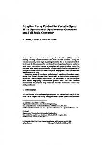
The key to any successful indoor thermal analysis lies upon the accuracy of the model of the indoor conditioned space within building and HVAC equipments. The simple hand-calculation methods were available to find out the cooling/heating load until the advent of computer simulation programs for HVAC systems in the mid of 1960s. The first simulation methods attempted were to imitate physical conditions by treating variable time as the independent [1]. Most of the earliest simulation methods were based on a white or mathematical (physical) models, which are preferred over other models such as a black box and gray box model because they are easy to analyse even though they are complex than others as shown in Figure 1.1. Model boxes in Figure 1.1 are based on the complexity versus the fidelity of the model or signal-to-noise ratio (SNR) [2].
Figure 1.1 Illustrate model staircase boxes with complexity and SNR
2
1.1.1 Mathematical model of HVAC system There are two types of the white box or mathematical model; the lumped and distributed parameter. The main advantage of a lumped parameter model is it is much easier to solve than a distributed model. The mathematical models are very popular for HVAC systems to represent the processing signal. The processes' signals are constructed based on physical and chemical laws of conservation, such as component, mass, momentum and energy balance. These laws describe the linking between the input and output which is transparently represented by a large number of mathematical equations. Furthermore, the mathematical model is a good tool to understand the behaviour of the indoor condition by describing the important relationships between the input and output of the HVAC system. In general, the modelling process of HVAC systems leads to dynamic, nonlinear, high thermal inertia, pure lag time, uncertain disturbance factors and very high-order models. The whole model can be described by several submodels to alleviate the complexity of the model [3]. These sub-model processes are related to fluid flow and heat-and-mass transfers between interfacing sub-models, which can be governed by mass, momentum, and energy conservation principles. These principles are usually expressed by differential equations, which may be implemented by time domain or S (frequency) domain where the S domain can be represented by a transfer function or state space function. The limitations of the early building mathematical models are mainly due to the limitation in the computer hardware since the models needed intensive computational process. But the situation is changing as computational tools capacity has improved by the evolution in software and hardware of computers. The recent mathematical models are being
3
developed to solve the large set of equations that also incorporate sub-models mathematical equations.
1.1.2 Black box model of HVAC system The concept of the black-box model is to fit transfer function model to the input/output real model data to yield coefficient polynomials that can be factored to provide resonance frequencies and characterizing of damping coefficients without knowledge of the internal working. Hence, it does not reflect any specific physical or mathematical structure of the existing behaviour in the real model. The mathematical representations of this model include time series such as Auto-regressive moving average (ARMA), Auto-regressive model structure with exogenous inputs (ARX), recurrent neural network models and recurrent fuzzy models. For real-time operation and control, the black-box models are simple enough. On the contrary, physical or mathematical modelling involves detailed analysis of the relationships between all parameters that affect the system. Due to the complex nature of HVAC systems and the large number of parameters involved, it is difficult to mathematically model the system [4]. Romero [5] mentioned that the mathematical models require detailed facility information that is sometimes hardly found. Therefore, the black box is the simplest solution, but at the same time has to be regularly updated as operation conditions changes. Thus, it cannot be used for prediction outside the range of the training data, and such models have poor performance in general.
1.1.3 Gray-box models of HVAC system Some physical processes of HVAC system are less transparently described where there is much physical insight available, but certain information is lacking. In this
4
case, mathematical models could be combined with black box models where the resulting model is called a gray box or hybrid model. Furthermore, some white box model of the HVAC system needs modification to provide better performance; this can be accomplished by using a gray-box technique to mimic the output of the whitebox analysis. This method is implemented by Leephakpreeda [6] when building a gray box model based on the white box model to predict indoor temperature. Some black box models for the HVAC system are modified to become gray box model to improve its performance as done by Zhao et al. [7] when they identified the nonlinear link model parameters by a neural network to represent heat exchanger. This means that the main function of a gray box is to improve the performance of the white or black box model.
1.2 The HVAC system Control The HVAC system capacity is designed for the extreme conditions where most of the operations are acting as a part load design due to the variables such as ambient temperature, solar loads, equipment and lighting loads, occupancy, etc. vary throughout the day. Therefore, the HVAC system will become unstable without the controller system to avoid overheating or overcooling in the space. The first requirement of HVAC system control design is it has to be stable at a closed-loop state. The nonlinearity and uncertainty in the HVAC systems are the two major difficulties that can make the design of stable control systems to be difficult. Nonlinearities act to reduce, or eliminate our ability to use tractable linear mathematics and uncertainties compel us to sacrifice performance in order to ensure adequate control over a range of plants behaviour. Furthermore, there are some
5
factors that make the HVAC control system designs difficult such as pure lag time, big thermal inertia, large-scale system and constraints. In order to overcome these factors, researchers used many types of control algorithms in HVAC systems. The most popular of these controllers (from the simplest to more complicated) are the cycling on-off or called two position or bangbang controller, traditional controller such as proportional, integral and derivative (PID) controller, modern controller such as linear quadratic regulator (LQR) and model predictive control (MPC) controller, model based control such as internal model control (IMC) and fault tolerant control (FTC) controller, robust controller such as H2 and H∞ controller and artificial intelligent (AI) controller such as artificial neural network (ANN), fuzzy logic control (FLC) and genetic algorithm (GA) etc. These controllers become further complicated by the new loadmanagement technologies and development of building and HVAC system over time, where it had taken natures of modernization. Therefore, the old controllers become feeble against these challenges of changes, resulting in some researchers applying some intelligent controller to their HVAC system, for example [8-14], that uses methods such as neural network (NN), fuzzy logic control, etc.
1.3 The HVAC system Simulation To reduce the design cost as well as the design process for testing and developing the HVAC systems, this study adopted simulation methods for modelling systems, result analyzing and controller design. Obtaining better performances of the simulated systems become easier [15] because of the progress of the digital computer has taken a quantum jump which allows the possibility for HVAC systems to be examined and assessed through model simulation [16].
6
There are three main driving forces influencing the simulation development process and its evolution [17]. a) the developments in computer software and hardware, b) the upturned understanding of the fundamental physical processes, and c) the expertise gained from constructing the previous generation of models. The influence of these three driving forces helped to solve probable areas of uncertainty and limitations by simulation methods. The observations on a synthetic HVAC system by simulation are referred to imitate the performance for a real system. In the numerical simulation, the equations of a model are converted into a computer program by a numerical algorithm. Using the computer to implement the algorithm is one of the most powerful and economical tools currently available for the design and analysis of complex systems such as HVAC system. The most early simulation work in HVAC system was sponsored by the American Society of Heating, Refrigerating, and Air-conditioning Engineers Inc. (ASHRAE) in the USA. There is a vast amount of specialized programs in the field of HVAC system such as TRNSYS [18], HVACSIM+ [19], IDA [20], SIMBAD [21], SPARK [22, 23], BEST [24], BLAST [25], EnergyPlus [26] and HAM-tools [27]. But each program has limited applicability because they are specific for only a particular range, not covering all the implementation range to complement certain calculations required for analysis or simulation. Furthermore, most of these programs are not suitable for modelling innovative building elements such as building integrated heating and cooling systems, solar walls and ventilated glass façades, as these have not been defined in the program [28, 29]. MATLAB and SimuLink from MathWorks are adopted in this study because they are appropriate and efficient
7
environment tools for designing and testing of modelling and controllers analysis in a simulation setting [30].
1.4 Problem Statement Until now, many HVAC system modeling approaches are made available and the techniques have become quite mature. But there is no combined model for the comprehensive HVAC system with subsystems in detail although the literature presented two types of HVAC system's model; steady-state models and unsteadystate models. The thermal comfort is a relative term for feeling and is very difficult to represent mathematically without the assistance of modern computers. Previous studies show that the human thermal feeling depends on human variables as well as environmental variables. The environmental variables are dry bulb temperature of conditioned air, humidity of air, air velocity and mean radiant temperature. The human variables are thermal resistance of clothes and activity level. To control the environmental variables within a comfort region, the HVAC hardware models and the whole building model are required to be integrated into one model, resulting in more complicated building model. The integration process will act to accumulate the defective characteristics of all the hardware and building models, which leads to the increase in the nonlinear characteristics of these systems. Some of these characteristics on the HVAC system control have been previously pointed out; nonlinear, pure lag time, big thermal inertia, uncertain disturbance factors, large scale system and constraints. Furthermore, the indoor thermal comfort is a function on the temperature and relative humidity in which they are coupled with each other. The conventional controller like PID which is widely used in HVAC system is
8
insufficient when dealing with these characteristics. One of the challenges of this study is to confront the control algorithm in a simulation environment with the above-mentioned problems. And the second challenge is to represent all of these characteristics in the models.
1.5 Research Objectives The goal of this research is to design TSFF intelligent control algorithm to provide the indoor thermal comfort within standard range, which depends on many controllable and uncontrollable parameters. To achieve this task, the fallowing objectives are stipulated:
To emulate the modelling of building and air handling units (AHU) through the development of physical empirical hybrid concept based on thermal and moisture dynamic phenomena.
To identify the indoor thermal comfort model by converting the empirical model into novel identification method based on Takagi-Sugeno (TS) fuzzy rules.
To design TSFF intelligent control algorithm to manipulate inherent characteristics of comprehensive model.
The first two objectives, which are development / enhancement of building, AHU and indoor environment models, will lead to investigation of new method for controller design, which minimizes the dependency on traditional models that are very simple in structure. Since simple building models are reduction of a real model, secondary dynamics is often neglected and unforeseen system changes reduces the accuracy of the model. On the other hand, these types of models are easy to implement by a simple control algorithm since most of the complex inherited
9
characteristics are excluded. This study is considering all these complex characteristics during HVAC system modelling such as a nonlinearity of the large scale system including pure lag time, big thermal inertia, uncertain disturbance factors and constraints. On the other hand, indoor thermal comfort is affected by both temperature and humidity which are inter-related between each other.
1.6 Scope of study The scope of this study is to cover the main goal of this research (indoor thermal comfort) that can be achieved by achieving the three objectives of the thesis. This is done by mathematically modelling the building, AHU and indoor thermal comfort and design applicable control algorithm capable of manipulating the developed models. The building and AHU can be divided into subsystems where each is modeled separately and then combined to form the overall system model. There are six attributes to the physical space that influence comfort; lighting, thermal, air humidity, acoustical, physical, and the psychosocial environment. Of these, only the thermal conditions and air humidity can be directly controlled by the HVAC system. Therefore, the construction of building models discussed in this thesis is based on these two attributes. And these attributes are closely related to the building and the air supplied to the building by AHU as shown in Figure 1.2.
Figure 1.2 The main fields of the HVAC system
10
1.7 Thesis outline The subsequent chapters are as follows; Chapter 2 provides information about literature researches regarding modelling of building, AHU and indoor thermal comfort as well as HVAC system control algorithms. These include discussion and related literature on the three objectives of the thesis and also references related to HVAC systems with nonlinearities, pure lag time, big thermal inertia, uncertain disturbance factors, large-scale system, constraints and uncertainty. Chapter 3 shows the modelling method in detail and how the two types of models are designed. The controller architecture and algorithm are explained in Chapter 4. The simulation for both the models and the controller are presented in Chapter 5, which provides the baseline of application and the validation of the results. Chapter 6 shows the results for the models and control performance and discussion on the results analyses. Conclusions and future works are given in Chapter 7, which provides a concise description of what has been achieved and what we can improve by recommendation for future works. The appendix provides the proof of the models' derivation that is repeatedly used in Chapters 5 and 6, and shows the details of the m-file program used in calculation and analysis of the study.
1.8 Summary This chapter has described the topics related to this study where it shows in general the types of a model and what are the advantages and disadvantages of each one of them, and it is clear from the introductory description that the gray box type is the best model type. This chapter also briefed the types of controllers applied on a HVAC system, and basically most of the controllers developed before the last decade are linear types, sparking evolution in nonlinear controllers over the past decade or
11
so. HVAC system simulation softwares are also presented in this chapter for the past and current decade where most of these programs are specialized in the specific scope of study. For this extensive study, it requires the usage of a comprehensive software such as Matlab. The problem statement section presented the main challenges that will be encountered through the proceeding to this study. The objectives of the study are clearly specified to solve the problem statements. Based on these objectives, the scope of study is specified, which is described in the subsequent chapters.
12
CHAPTER 2
HVAC SYSTEM LITERATURE REVIEW
2.0 Introduction Since the ancient time, human beings have sought to build a hut in order to alleviate the harshness of the climate to provide a suitable indoor environment. The evolution of research has been reflected on the evolution of indoor environment by development and enhancement of buildings and HVAC equipments. In general, research on indoor environment can be divided into two main categories; designoriented research and research-oriented design as explained by Fallman [31]. This study followed the second category where it depends on the previous research outcomes to develop design that enhances the indoor thermal comfort. This category is further divided into two fields of study; control and modelling research orientated and simulation design research orientated. The main body of this thesis is based on these fields where the first three chapters are related to the investigation field while the later chapters are related to the implementation field as shown in Figure 2.1.
13
Figure 2.1 The main framework of the thesis
14
2.1 Building and AHU model The commercial and residential buildings are facing a new era of a growing demand for intelligent buildings worldwide. Intelligent buildings are referred to as energy and water saving and provide healthy environmental. The first intelligent building was introduced in the late 1970s when buildings were equipped with IT equipments [32]. The developments of improved building and AHU models are essential to meet the requirements of an intelligent building [33].
2.1.1 The evolution of modelling HVAC system Building and AHU modelling has been used for decades to help HVAC system scientists design, construct and operate HVAC systems. The pioneering development in the building and the HVAC equipment industry is the heat conduction equation model by Joseph Fourier published in 1822, which is the most cited model [e.g.3437]. The earlier simulation work in building structure by Stephenson and Mitalas [38, 39] on the response factor method significantly improved the modeling of transient heat transfer through the slabs, opaque fabric and the heat transfer between internal surfaces and the room air. The heat balance approaches were introduced in the 1970s [40] to enable a more rigorous treatment of building loads. Rather than utilizing weighting factors to characterize the thermal response of the room air due to solar incident, internal gains, and heat transfer through the fabric, instead, the heat balance methodology solves heat balances for the room air and at the surfaces of fabric components. Since its first prototype was developed over two decades ago, the building model simulation system has been in a constant state of evolution and renewal. Numerical
15
discretization and simultaneous solution techniques were developed as a higherresolution alternative to the response factor methods [41]. Essentially, this approach extends the concept of the heat balance methodology to all relevant building and plant components. More complex and rigorous methods for modeling HVAC systems were introduced in the 1980s. Transient models and more fundamental approaches were developed [42] as alternatives to the traditional approach which performed mass and energy balances on pre-configured templates of common HVAC systems. The delivery of training and the production of learning materials [43] are also receiving increased attention. Additionally, many validation exercises have been conducted [44] and test procedures developed [45] to assess, improve, and demonstrate the integrity of simulation tools. The literature presented two types of HVAC system's model; steady-state models, which are extensively presented such as [46-51], and unsteady-state models presented by [52, 53]. Unsteady-state models can be further categorized into two extreme modeling approaches. The first approach, called physical or mathematical models, builds up models entirely based on universal laws, physical laws and principles [54]. The second approach, called empirical or black box models, constructs models entirely based on experiments or data [55-57].
2.1.2 Mathematical model Mathematical models have been widely used in areas as diverse as engineering, economics, medicine, ecology and agriculture for many kinds of different purposes to satisfy scientific curiosity, prediction, control, fault diagnosis and inadequacies, simulation and operator training.
16
In the field of HVAC system modelling, the most complicated model part is the building model. This is because components that need to be modelled for building are not limited to building construction, such as roof, walls, floor slab, windows and external shading. Internal loads such as the activity within the space, the number of people, and the heat gain from lighting must also be modelled as well. The subdivision of the building model is an extensive scope of the HVAC models' field, and there are rarely studies that include the entirely scope of a building model. For example, Lu [58] studied the transmission of heat and moisture throughout the walls, roofs and ceilings to estimate the indoor air temperature and humidity. He didn’t consider the transmission of heat and moisture throughout ventilation, filtration (doors and windows) and internal load. Furthermore, the moisture conservation equation used assumed the temperature to be the same in all the phases. He constructed his model by applying the conservation of mass and energy theory based on the fundamental thermodynamic relations. For mass conservation law, he implemented this in moisture transmission by applying Darcy’s law and Fick’s law. For energy, he implemented Fourier’s law. He used distributed white box model where partial differential equations is discretized in space by using finite element with time marching scheme and Crank-Nicolson scheme. On the other hand, Ghiaus and Hazyuk [59] used mathematical model to estimate the heating load in dynamic simulation by using steady-state heat balance for normalized outdoor conditions. They applied the superposition theorem for electrical circuits to obtain their model's parameters. And they assumed that the thermal model of the building is linear, thermal capacity of the wall and the indoor air is lumped and considered that the time series of disturbances (such as weather, internal loads) and occupational programs are known because they used model predictive control (MPC)
17
which proposed an unconstrained optimal control algorithm to solve the load estimation problem. They obviously have imposed many assumptions to facilitate the calculations of heating load, which leads to lack of accuracy in the results. In addition, they used a single input single output (SISO) type model that doesn’t consider the moisture transmission, an important element in deciding thermal comfort. For the air handling unit (AHU) mathematical model, Wang et al. [60- 63] built models of heat exchanger for air handling unit based on the conservation of energy and applied thermal balance equation on control volume for heat exchanger. This model is characterized as a SISO model since it does not take into account the effect of the mixing air chamber and assumed the temperature of air supplied to conditioned space is equal to the surface temperature of heat exchanger. Furthermore, they neglected the humidity of the moisture air supplied to the conditioned space because they do not want to include the effectiveness of humidity variation on thermal comfort. Therefore, they supposed that the type of cooling coil is of a dry type and there is no indoor latent load.
2.1.3 Black box model The physical model involves detailed study of the relationships between all parameters that affect the hygrothermal (the variation of humidity and temperature) system. Due to the complex nature of hygrothermal systems and the large number of parameters involved, physical modelling has become more complicated in application. Usage of black box model is sometimes preferred because it is straightforward to construct and there is no need to have knowledge of the system’s internal structure. 18
Mustafaraj et al. [64] identified the humidity and thermal behaviour models of an office in a modern commercial building by using different methods of the black box model such as Box–Jenkins (BJ), autoregressive with external inputs (ARX), autoregressive moving average exogenous (ARMAX) structure and output error (OE) models. They adopted linear parametric models to predict room temperature and relative humidity for different time scales. The linear model is adopted to obtain a simple and low number of model parameters, but this caused downbeat on the accuracy, especially in the representation of the heat storage or flywheel effect on the instantaneous load. In this group of models, they found out that BJ model is suitable for the winter season where the ARMAX and ARX models give good results for the summer and autumn seasons and OE is appropriate for summer season. This means that there is no specific model can represent indoor temperature and humidity for all four seasons. Furthermore, Mustafaraj et al. [65] created the neural network based nonlinear autoregressive model with external inputs (NNARX) model, which is suitable to predict indoor office temperature and relative humidity for summer season. The learning of NNARX model is done off-line because this type of model is well known for having a sluggish learning process. On top of this, they used Optimal Brain Surgeon (OBS) strategy which made the learning much slower, so it is not suitable to apply online learning process [66]. Yiu and Wang [67] created a generic SISO and MIMO black box model for AHU. The ARX and ARMAX structures are used, where their parameters are identified by using the recursive extended least squares (RELS) method. In general, the selection of model structure, between SISO and MIMO as well as between ARX and ARMAX, is a compromise between model simplicity and accuracy. The accuracy of the anticipated model outputs is in contrary with simplicity and the time period of
19
updating weight. Furthermore, the more the accurate the ARMAX structure is, the more complex it becomes, which will also yield more residual white noise. Barbosa and Mendes [68] integrated the works of a group of researchers in order to obtain a comprehensive model, for the chiller model is quoted from CA [69] by applying empirical equations based on regression functions. The cooling tower model used is based on Merkel’s theory for the mass and sensitive heat transfer between the air and water in a counter flow cooling tower. The pumps and fans model are quoted from Brandemuehl et al. [70] where power for variable flow is calculated from a regression of part-load power consumption as a function of part load flow with the assumption that motor efficiency is constant. For the cooling and dehumidification coil model, there are three possible conditions for the coil: completely dry, partially wet or completely wet. The model for all three conditions is quoted from Elmahdy and Biggs [71] based on coil outside surface temperature and air dew-point temperature. The room building model for heat and moisture transfer is based on the Philip and DeVries theory, which solves the partial differential governing equations for room control volume within the porous building element, which is quoted from Mendes et al. [72], where it is assumed that the water vapour behaves like a perfect gas and the vapour exchanged between the wall and the air is in a linear function of the differences between the temperature and moisture content.
2.1.4 Gray box model The Grey box model, sometimes called semi-physical or hybrid model is created by a combination of physical and empirical models, which is to compensate for their deficiencies as individual approaches.
20
In some gray box modelling, the model structures are derived mathematically from physical or thermodynamic principles, while their parameters are determined from catalogue, commissioning or operating data. This is what Braun et al. [73] and Wang et al. [74] did when they developed an effective model through introducing the idea of air saturation specific heat. Catalogue data at an operating condition are used to obtain the number of transfer units, which is then employed to obtain the performance at other operating conditions. Based on the same concept of Braun et al., Wang et al. [75] built their gray box model for predicting the performance of chilled water cooling coils in a static state. The mathematical part they built was based on heat transfer mechanism and the energy balance principle. A model with no more than three characteristic parameters that represent the lumped geometric terms was developed. Procedures for determining the unknown parameters using commissioning or catalogue information by linear or nonlinear least squares methods are used. Using this method, the model captures the inherent nonlinear characters of the AHU. Both Braun’s and Wang’s models have a high level of uncertainties because they evaluated models parameters depending on catalogue and operation data where most of these data are estimated from ideal operation conditions. Some data are measured from the real operation but these parameters value will eventually change due to the aging of the HVAC system. Meanwhile, Ghiaus et al. [76] used a gray box model to identify the AHU by imposing in the mathematical part that air temperature difference occurs in cooling coils and the humidity ratio difference occurs in the humidifier only, meaning that the cooling coil is of dry type, and there is no change in the air temperature through the humidifier. This is to separate the transfer functions for each element in order to overcome the coupling between the temperature and humidity, where the parameters
21
of the discrete form of these models are then experimentally identified. It is obvious that the assumptions made by the authors are too unrealistic and cannot be achieved except in some rare cases. This lead to avoidable inaccuracy in the model’s output data.
2.2 Indoor Thermal comfort model Indoor thermal comfort model is a major indicator for an HVAC system which is designed based on a number of variables that physiologically affect human comfort. This based on the fact that human body loose heat continually due to metabolized food. The rate of body heat loss is the factor that determines whether one feels cold or hot. The objective of literatures on human thermal comfort is to substantiate the criterion of thermal comfort for evaluating the indoor thermal sensation. The researchers are proceeded to identify the variables which affected human comfort over the past three decades.
2.2.1 The evolution of thermal comfort The climate criteria of the thermal comfort index is continuously/gradually developed over time; such as wet bulb temperature (Tw) [77], effective temperature (ET) [78], operative temperature (OpT) [79], thermal acceptance ratio (TAR) [80], wet bulb dry temperature (WBDT) [81], and so on. However, the major and widely used thermal comfort index is the Predicted Mean Vote (PMV) index. The PMV model is developed by Fanger in 1972 [82]. Based on this model, a person is said to be in thermal comfort based on three parameters: 1. the body is in heat balance; 2. sweat rate is within comfort limits; and 3. mean skin temperature is within comfort
22
limits [83]. Based on these parameters, Fanger established his empirical model by using the estimation of the expected average vote of a panel of evaluators. There are also criteria not related to climate which are also developed over time. These criteria depend on variables that can affect how comfortable a person feels in a given situation, such as: age [84-86], acclimatisation, clothing, sex [87-90], activity and health [91, 92], and subcutaneous fat. Furthermore, the geographic location criterion could have an influence on thermal comfort. Parsons [91] argues that this is not being shown to be the case in some research such as [92, 93]. Thermal comfort also depends on the activity, metabolism of physiology and thermoregulatory system of the body [94-99]. However, the variation of the metabolism and activity in residential buildings is hard to predict compared to commercial buildings. The same can be said about the type of clothing worn in the residential buildings. These factors make the criteria for comfort conditions difficult, making it more difficult to predict indoor thermal comfort in residential buildings compared to those in commercial buildings.
2.2.2 The predicted mean vote (PMV) index There are numerous mathematical relationships to represent the thermal comfort, as previously mentioned. In 1967, Fanger studied the physiological processes of a human when they are close to steady-state condition to define the real comfort equation. His studies [100] initiated with the assumption that physiological processes influencing heat balance can be determined from the mean skin temperature and sweat rate as a function of activity level. Then he used data from an investigation by McNall et al. [101] to obtain a linear relationship between sweat rate and activity levels and proceed with 23
an investigation to obtain a linear relationship between the mean skin temperature and activity levels. These two linear relationships are used in heat balance equations to formulate a thermal comfort equation to describe all integrations of the six PMV input factors that result in a neutral thermal sensation. The thermal comfort equation is corrected by combining data from Nevins et al. [102], taking into account situations where human do not feel neutral [82]. At that time, the Fanger model was accepted to be the closest one to the real behavior of the indoor actual model, and that is the reason why it is adopted in ASHRAE Standard 55-92 [103] and ISO-7730 [104]. Therefore, it is widely used for PMV calculations. The PMV is dependent on two variables. The first variable is the composite of skin temperature and the body's core temperature to give a sensation of thermal neutrality. The second variable is the body's energy balance: heat lost from the body should be equal to the heat produced by the metabolism. The range value of PMV is from -3 to +3, where a cold sensation is shown as a negative value, the comfort situation is close to zero and hot sensation is shown as a positive value. The PMV is also used to predict the number of people likely to feel uncomfortable as a cooling or warming feeling. This feeling is cited under the Predicted Percentage of Dissatisfied (PPD) index. The output of the PPD is classified into two categories, comfortable and uncomfortable, according to human sensation. The variation behavior of PPD versus PMV is imperative for the HVAC system to control indoor desired conditions as implemented by many researchers [54, 105109].
24
2.2.3 PMV models The process of calculations and obtaining PMV value from Fanger’s model requires a long time since the number of input variables takes a long routine due to some of them require iterations. For iteration loops, if the initial guess of the input variables is far from the root, it might take a long time for it to converge to the root. The Fanger’s model has been used directly by using a spreadsheet or numerical methods to obtain a thermal comfort index [110-112], while others converted it into a blackbox model [113-116]. Since Fanger’s model involves implicit equation, calculation of the PMV manually by a spreadsheet will take a long time due to the presence of an iteration process. Furthermore, the main two disadvantages of a spreadsheet as follow: - First it does not have any built-in transaction-control capabilities, meaning that any error occurred on the spreadsheet cannot be repaired; in this case, the spreadsheet must be restored from a backup. Second, is doesn’t capture some of the model characteristics such as a thermal dependence [117]. Therefore, since the Fanger’s or PMV equation is not an explicit function of the six factors that affect thermal sensation and to avoid the iterative process, the implicit calculation by black box model is identified to predict PMV value by many researchers such as Hamdi et al. [118]. Furthermore, the Fanger’s equation is cumbersome to calculate the PMV index and is not suitable for feedback control of HVAC systems [105, 119]. The black box model of the thermal sensation index which is designed by Hamdi et. al. [118] is based on the basis of neuro-fuzzy logic theory by learning Fanger’s equation. The neuro-fuzzy model of thermal sensation provides a quick and direct calculation of the thermal sensation index which makes it an attractive index for
25
feedback control of HVAC systems. But Hamdi used Mamdani’s fuzzy inference system's model, where this model requires a large number of rules to meet the asymptotic representation of the real Fanger’s model. Furthermore, he used backpropagation algorithm to tune the fuzzy model where this type of algorithm has notorious long training time requirement [120]. On the other hand, many researchers used black box models by employing neural network to identify the PMV model [121, 122]. Mistry and Nair [121] used feedforward neural network model, which allows real time determination of the thermal sensation index quantitatively. They also contributed to the field of function approximation for thermal comfort index by modeling of PMV index using back propagation neural networks. Out of the six input factors, two input are considered as constants and corresponding to these constant input factors, correction networks have been added in the neural network structural design. Atthajariyakul and Leepahakpreeda [122] developed feed-forward neural network architecture model to capture the relations of the conventional thermal sensation model by Fanger, also quantitatively. They also use back propagation algorithm in the training process to tune the two hidden layers' weights of the PMV model structure. However, this model showed significant margin of error when its outputs are compared with Fanger’s model outputs within 9 hours at day. Other researchers such as Lute and Paassen [123] described the indoor PMV by an ARMAX model, which estimates the indoor thermal comfort by a recursive estimation algorithm. The disadvantage of this ARMAX model is it becomes very complex by increasing the model order when converted into a MIMO model [124]. To reduce the complexity of model, Lute and Paassen [123] fixed all the inputs’ parameters at certain values and only used the temperature as the input. They also
26
assumed the indoor air temperature and the mean radiant temperature to be the same to convert the model to SISO type. This approach leads to a simple model where its output is easy to control using a linear predictive control (LPC). But this affects the model accuracy and does not represent the real indoor PMV. In the last few years, adaptive thermal comfort for PMV model is proposed by some researchers [125-131] to represent a dynamic indoor thermal sensation, which is determined by the combination of three criteria: behavior adaptation, physiological adaptation and psychological adaptation [132]. This type of model is fairly capable of representing the dynamic situation of the indoor thermal sensation, but it does not include human clothing or activity or the four classical thermal parameters that have a well-known impact on the human heat balance and therefore on the thermal sensation [133]. Another great disadvantage of the adaptive thermal model is its application range, which is limited to workspaces and offices only, while the Fanger’s PMV model can be applied throughout to almost all types of buildings [134]. In addition, adaptive models are not suitable for energy saving due to their static value for a daily period [54]. Therefore, it can be said that Fanger’s thermal comfort model represents a deep analysis that relates variables that contribute in thermal sensation [135].
2.3 HVAC System Control The main objective of the HVAC system control is to maintain the design condition of thermal comfort in conditioned space. Other objectives include; reducing human labor, minimizing energy consumption and costs, keeping equipment operation at safe levels and so on. To achieve the main objective of the HVAC system control,
27
there must be at least one controllable variable to be controlled by a controller device, which is developed through time.
2.3.1 The evolution of HVAC system control Basically, there are two types of controls theory; open loop or closed loop control. Open loop or feed forward control is a system without monitoring whether the control system is working effectively or not. In the closed loop or feedback control system, the controller responds to the error between the controlled variable and the set-point. The closed loop control can be broadly classified into two categories; two position control (On-Off) and continuous control. The first closed loop control in the HVAC system was a regulator space-heating system using bimetallic strip. The bimetallic strip was the first device used; it controlled the boiler output using a combustion air damper to control the rate of combustion. This device was known as a regulator, which is used again to control steam radiators and steam heating coils [136]. Dr. Andrew Ure (1778 – 1857) was the first person to call his regulator a thermostat, which is soon used to control temperatures in railway cars, incubators, restaurants, and theatres [137]. Two other devices were developed to compete with the bimetallic strip. They are mercury thermometer column, mercury switch, capillary thermostat and proportional thermostat, which are still used to control countless processes in HVAC systems [138, 139]. Early controls for comfort air conditioning systems were used to maintain the desired supply air temperature in USA Capitol building since 1928 using pneumatic type control [140]. Shavit [141] indicated the possibility of using a thermocouple for remote monitoring of conditioned space temperature, which is implemented in the first centralize monitoring system with a remote set point change 28
and central panel installed in the White House in 1950 by using pneumatic local control systems. Shavit also said that in Dallas, Texas, the first on-line computer was introduced 1967, where the first set of energy conservation software was installed that includes chiller optimization, enthalpy control, optimum start/stop, demand limit, reset according to the zone of highest demand and night purge. Another significant milestone occurred in 1970, when solid-state components improved the scanning process and serial transmission as well as reduced many wires in the trunk wiring to a single pair. In 1981, the first microprocessor-based direct digital control (DDC) which used software programmed into circuits to affect control logic was introduced [140]. The most common algorithm for control logic appropriate for HVAC system is called proportional plus integral plus derivative (PID). The control action logic of the PID adds a predictive element to the control response, which takes care of sudden changes in deviation due to disturbances. This controller combines proportional control with two additional adjustments, which helps the HVAC system to compensate automatically for changes in the conditioned space.
2.3.2 PID control for HVAC system PID controllers are widely used in HVAC systems field because of their simple structure and their relative effectiveness, which can be easily understood and executed by practical implementations [142]. However, PID controllers are reliable only if the parameters of the system under consideration do not vary too much. On the other hand, variations in the operating condition of the HVAC system will cause changes in the parameters of the system. These variations can be due to many factors such as water’s chilled temperature, weather and occupancy level, which changes from day to night. In short, the system is time variable and highly nonlinear. For 29
these reasons, even for a single HVAC system, the use of a constant set of PID parameters will not give best results [143, 144]. To obtain good PID control performance, the PID parameters should be tuned continuously, which is timeconsuming and dependent on the experience of the one who adjusts them. Furthermore, despite the non-stop continuous research on improving PID algorithms, requirements for high product quality, subsystem unification and energy integration have resulted in nonlinearity and pure lag time for most of modern HVAC systems. Some researchers have incorporated PID with other algorithms to provide a new hybrid controller to cover the wide range of HVAC system operation conditions [145, 146]. Several of these hybrid controllers are capable of managing two controlled variable such as the controller developed by Paris et al. [145] when they combined two parallel control structures based on PID and fuzzy controllers. The hybridization structure of the PID-fuzzy for the indoor temperature controller allowed efficient management of energy resources in buildings. By this combination, they took advantage of the properties of the two structures to control the indoor temperature and energy consumption without referring to the variation of indoor humidity and other factors affecting the thermal comfort which causes the controller's efficiency degradation or may also cause disability to control the plant system. Meanwhile, Xu et al. [146] developed a hierarchical structure control scheme that incorporates generalized predictive control (GPC) into the PID controller. This is to address the issues of advanced tuning methods normally lack explicit specifications and the AHU operators unfamiliarity with the parameters tuning. This structure control strategy consists of two levels, a basic level and an optimization level, for the basic level is represented by the conventional PID controller, and the optimization
30
level is used to vary the gain values of the PID controller. This type of controller is implemented in modeling of cooling coil for AHU by using controlled autoregressive and integrated moving average model (CARIMA) to control supply air temperature and flow rate without looking into air humidity, which is difficult to control since it is coupled with temperature. The process of PID hybridization with a cascade control structure is adopted by many researchers in HVAC systems since it is efficient and transparent when compared with the single-loop PID controller since these controllers have cascade control algorithm to evaluate the data from the sensor network and manipulate AHU parameters such as supply air temperature, air and chilled water flow rate [61, 147151]. However, the tuning procedure of hybrid PID-cascade controller is tedious and it is difficult to obtain the inner and outer loop PID parameters simultaneously. To avoid tuning difficulty, some researchers adopted hybrid PID auto-tune cascade control systems, for example Song et at. [147] when they established a model based on PI tuning rules for Ziegler-Nichols method which is applied to tune the inner loop, and the outer loop tuning is applied by model matching algorithm to obtain the PID control parameters for the overall system performance. Both inner loop and outer loop process model parameters are identified using relay feedback by utilizing the physical properties of the proposed structure. This method is straightforward for cascade control structure with the possibility to be integrated into an existing autotuning system to control the overall system performance. The disadvantage of this structure is it can be implemented only with SISO model. Other researchers [61, 148-151] implemented hybrid PID-cascade control to improve control system performance over single-loop PID control whenever disturbances affect a measurable intermediate for inner loop controlled variable or secondary
31
process output that directly affects the primary process (outer loop) output which is the main controlled variable. Furthermore, the hybrid PID-cascade control system has advantages over PID single loop in anti-jamming capability, rapidity, flexibility and quality control [151]. From previous literature, it is obvious that both single-loop PID and hybrid controller types are suitable for SISO system plants. However, requirements for high product quality, subsystem unification and energy integration have resulted in nonlinearity and pure lag time for most of the modern HVAC systems. These main characteristics have rendered many PID tuning techniques as insufficient for dealing with these modern HVAC systems, which are categorized as a Multi-Input Multi-Output (MIMO) process [152, 153]. Furthermore, the tuning of PID parameters in MIMO plants is difficult to obtain because tuning the parameters of one loop affects the performance of other loops, occasionally destabilizing the entire system. Therefore, most studies in the field of the HVAC system control tends to belong to artificial intelligence; neural network (NN) [154, 156], fuzzy control [10, 154], adaptive fuzzy neural network [8-12], etc.
2.3.3 Fuzzy logic control for HVAC system Fuzzy logic imitates human intuitive thinking by using a series of Zadeh’s fuzzy set, almost intuitive, if-then rules to define control actions. Zadeh’s fuzzy set theory [157] is a foundation of fuzzy logic control [158], and the first application of Zadeh’s theory was developed by Mamdani in 1974, when he designed an experimental fuzzy control system for a boiler and steam engine combination by synthesizing a set of linguistic control rules obtained from experienced human operators [159].
32
Fuzzy logic controller operates similarly with PID conventional controller, but able to manage complex control problems through heuristics and mathematical models provided by fuzzy logic, rather than via mathematical equations provided by PID algorithm. This is useful for controlling nonlinear systems by presenting the essential knowledge of the dynamics nonlinear systems behaviour in the form of a linguistic rule base. The fuzzy logic control is used in HVAC systems for its capability in dealing with non-linearity as well as its capability to handle MIMO plants. Moreover, in most cases, fuzzy logic controllers are used because they are characterized by their flexibility and intuitive use [160]. Two types of fuzzy inference system (FIS) models, Mamdani FIS and Sugeno FIS, are widely used in various applications [161]. The differences between these two FIS models befall in the consequents of their fuzzy rules, differing in their aggregation and defuzzification procedures. Researchers found that Sugeno FIS runs faster, is more dynamic to input changes and is more economical in the number of input fuzzy sets compared to Mamdani FIS. It is also observed that Sugeno FIS is more accurate since the results that were generated were closer to what was expected [162-164]. Jassbi [165] concluded that Sugeno FIS performs better than Mamdani FIS with respect to noisy input data. Furthermore, Sugeno FIS is more responsive and that is due to the fact that when the noise becomes too high (i.e. when the input data has drastically changed), Sugeno FIS reacts more strongly and its response is more realistic. In recent years, the learning methods based on using fuzzy control emerged as a vital tool in applications used to control nonlinear systems, including HVAC systems. For large scale HVAC systems, iterative tuning controller makes a system better by obtaining minimum cost on a system level [166].
33
The first fuzzy control application in the HVAC system was in late 1989 by Imaiida et. al. [167] when he developed a fuzzy logic control system using Mamdani FIS, which is designed to control temperature in commercial buildings, achieving a high comfort level with energy savings up to 25%. The dominant majorities of the fuzzy controls implemented on HVAC system were of Mamdani FIS type because it is straightforward and can be smoothly applied. On the contrary, Sugeno FIS type, which was adopted by some of the researchers [168170] requires a proper mathematical equation which makes it difficult to tune its parameters instead of consequent fuzzy rule in Mamdani FIS. Sousa et al. [168] was the earliest to implement Takagi–Sugeno (TS) fuzzy control in the HVAC system's field when he presented a sophisticated approach of predictive TS control tested on temperature control in an air-conditioning system. He demonstrated that the TS control requires fewer computations and achieves better performance than a nonlinear predictive control scheme based on iterative numerical optimization. He was using offline tuning by employing a least-squares method to estimate consequent parameters. Ghiaus [169] designed TS fuzzy control based on an identification fuzzy model then demonstrated that the nonlinearity of the heat exchange process can be well identified by a rather simple fuzzy scheme and showed that the fuzzy control resulted in improved performance and eliminated the offline retuning process required by the classical PID controller. However, the variable airflow rate which account for much of the nonlinearity and time varying characteristics in variable air volume (VAV) scheme was not considered in the work. He also concluded that the advantage of fuzzy controller resides in the easiness of understanding and including linguistic scheduling and expert type knowledge; or based on Lotfi Zadeh’s words, “in almost
34
every case you can build the same product without fuzzy logic, but fuzzy is faster and cheaper.” He et al. [170] used TS fuzzy models for AHU in HVAC systems based on a multiple model predictive control (MMPC) strategy. The controller system was constructed by a hierarchical two-level structure. The higher level was a fuzzy partition based on AHU operating range to schedule the fuzzy weights of local models in lower level, while the lower level was composed of a set of TS models based on the relation between manipulated inputs and system outputs corresponding to the higher level. He assumed that the temperature of the chilled water is constant, and the airflow rate varies in correspondence to the cooling load demand of the conditioned space. He used offline tuning to identify the consequent parameters for each cluster by using the stable-state Kalman filter method [171].
2.4 The Shortcoming in Previous Works and Alternatives From the reading through the literature in the topics of this research’s objectives which are summarized in the previous sections, faces some shortcomings that prevent the possibility to be implemented in the simulation environment. Thus, it can be concluded that the most important discouraging gaps to implement the analysis simulation properly and accurately for each objective are listed as follows:
2.4.1 Modelling of building and AHU There are a lot of deficiencies for each of the model studied that needs to be addressed. These deficiencies resulted from various simplifying assumptions to reduce the complexity of thermal interactions, unmeasured disturbances, uncertainty
35
in thermal properties of structural elements and other parameters which makes it quite a challenge to obtain reliable analytical models. The most prominent shortcoming in this area of studies is the fact that there is no model that includes both building and AHU with all the details. The other shortcoming is the existing building models do not represent the lag time cooling load and solar gains incident on the surfaces of wall, roof and window. In addition, the AHU model represented only the cooling coil without pre-cooling coil and neglected the effectiveness of air mixing chamber. Furthermore, there are some studies where the models are simplified, eliminating many of the important features such as humidity transmission, the change of air temperature through humidifier. Besides, most of the literature of previous works presented SISO type model which is easy to manipulate using linear controller. And the most important of all, a lot of studies assume that the cooling coil is dry, which is contrary to the reality. To address these shortcomings in the existing model, the following building and AHU model procedures are suggested for this study:
1) Use a physical-empirical hybrid modelling to describe the HVAC with its various thermal inertia parts. 2) Systematize the HVAC system into five subsystems to reduce the complexity of the modelling process. 3) Use the variable air volume (VAV) which is friendly with an empirical residential load factor (RLF) method for thermal load's calculations to enhance energy savings. 4) Use pre-cooling coil to control indoor humidity and such method results in reducing energy waste.
36
2.4.2 Modelling of indoor thermal comfort From literature review, it is noted that there are a lot of thermal comfort standards, but apparently Fanger’s PMV index is the closest to reality. Despite the importance of the subject concerning PMV model and its impact on the indoor thermal comfort, only a few publications in the literature can be found. These publications have many shortcomings that affect the outcome precision and the most important shortcomings are as follows: First the models were built in the form of black box type and hence it is difficult to analyze the processes mathematically such as prediction and extrapolation. The other shortcoming is most of the models used back propagation algorithm, which is slow in the learning process, making it difficult to be used in the online tuning. The literature of previous works also clarified that in recent years, adopted adaptive PMV model is used in many studies, which can be characterized by having small dynamic properties but at the same time neglects a lot of features that affect human comfort. For example, it does not include human clothing or activity or the four classical thermal parameters that have a well-known impact on the human heat balance and therefore on the thermal sensation. Its application range is limited to only workspaces and offices and is not suitable for energy saving due to its static value for a daily period. Based on these shortcomings, the study proposes the development of a comprehensive model with the following specifications:
1) Usage of the PMV index model which is suitable to be target set values for the indoor conditioned space rather than temperature because the PMV changes dynamically. 2) Building of a hybrid RLF-PMV model to properly control indoor thermal comfort in HVAC systems.
37
3) Usage of a white-box fuzzy PMV predictive indicators model to evaluate indoor thermal comfort. 4) Usage of the clustering concept of learning data set to reduce the number of rules and number of iterations and provide small margin error when compared with other methods. 5) Usage of Takagi-Sugeno model tuned by Gauss-Newton nonlinear regression algorithm for obtaining model’s parameters layer.
2.4.3 The control algorithms From literature review, it is found that the classical controllers such as PID are used widely in HVAC systems, although they are limited to the usage of the first order or second order plus time delay models to represent process dynamics [170]. However, as explained earlier, the HVAC model is a sophisticated MIMO model of a 13th order and therefore classical control strategies like a PID controller will fail to control it effectively. Furthermore, the PID controllers are reliable only if the parameters of the system under consideration do not vary too much. On the other hand, variations in the operating condition of the HVAC system will cause change in the parameters of the system. The first shortcoming in the most intelligent controllers available is they use temperature as a reference signal while the temperature itself does not represent the thermal sensation. Recent studies showed that the controlled variable PMV can be fitted (optimized) by the controller according to the amount of impact on the reference output. Therefore, using the PMV index as the target set value for the indoor conditioned space is a 38
better and more suitable choice than using temperature because the PMV changes dynamically so as to suit the constantly changing indoor environment, and this will be useful to HVAC control systems aimed at both controlling thermal comfort and energy consumption [172]. In addition to the use of temperature as a signal reference, it was noted that the identifications of TS models in the literature are tuned by only offline methods such as least-squares, PID or stable-state Kalman filter. That resulted in limitations on the valid input ranges for the models that are reflected on the performance of controllers and accuracy of the plant's outputs. Furthermore, the conventional fuzzy controllers such as Mamdani and TS fixed parameters use the feedback principle, which is characterized as slow for the indoor responses. The solutions to these shortcomings are that the new proposed controller will have following specifications:
1) Designing of an auto-tuned Takagi-Sugeno Fuzzy Forward controller to control thermal comfort in HVAC system. 2) Using the GNMNR algorithm for offline model training and the gradient algorithm for online controller tuning. 3) Using memory layers structure for the parameters of PMV sensors and controller models for faster calculations. 4) Adopting predicted mean vote to avoid thermal sensitivity and temperaturehumidity coupling, and to save energy.
39
2.5 Summary This chapter has reviewed numerous previous works related to each of the 3 objectives of this research to guide the study to develop the best and rational solutions for the problem statements of the current HVAC system. Through literature review which is summarized by this chapter for different types of model for HVAC system, a lot of advantages, disadvantages and shortcomings of the current models have been discovered. The review of the models' literatures are aimed at figuring out which type of model is the most suitable to represent the behaviour of the real HVAC system. By displaying the advantages and disadvantages of each of the three model types, it became evident that the gray box model has many features which discriminates it from the other models by closely representing the real behaviour of an HVAC system. Meanwhile, from the literature, the representation of the indoor thermal comfort is best represented by Fanger’s formula which is the closest to reality. And because of this formula being implicit, mathematically complicated and includes iterations process, there is a need to convert it into an explicit model. The methods of converting the implicit formula into an explicit model are different from one researcher to another; this chapter reviewed the features of each method, showed the general shortcomings for each method, and suggests an alternative method. Review on the existing controller algorithms of the common and widely used controllers in the field of HVAC system was also conducted. It is found that the classical controllers are dominant in this field, in spite of their inability to manage the modern buildings and indoor conditioned space to meet the desired requirements for thermal comfort and energy saving. The modern and intelligent controller algorithms are advent in the last few decades. They improved the performance of HVAC system
40
to control indoor thermal comfort, resulting in decline in the usage of the classical controllers. This improvement in the controller’s performance is continuing despite the increase of the complexity of buildings and HVAC system equipments, which produce the non-linearity and other undesirable characteristics. The literature review explained that intelligent controllers are proven to be important to improve the efficiency of HVAC system compared with other controllers, but there is a difference in the types and the structure of each type of these controllers. The fuzzy logic control algorithm type presented in the literature review is the most suitable for HVAC system because of its flexible characteristic and intuitive use.
41
CHAPTER 3
MODELLING OF HVAC SYSTEM
3.0 Introduction This chapter and the next chapter describe the proposed modifications in the design of HVAC system, and its control algorithm based on the shortcomings discussed in the previous chapter. The modifications of the HVAC system modelling presented in this chapter are based on reorganizing of the subsystem models. The first model for the HVAC system is divided into two parts; building and AHU model and indoor thermal comfort model. The building and AHU model adapted is based on hybridization between two methods; physical and empirical methods, depends on the thermal inertia quantity. Physical laws are used to build a sub-model for subsystems that have low thermal inertia while the empirical method is used to build a sub-model for subsystems with high thermal inertia. The empirical method used is the residential load factor (RLF). The second model is to evaluate indoor thermal comfort situations using predicted mean vote (PMV) and predicted percentage of dissatisfaction (PPD) indicators. These indicators are identified by a Takagi-Sugeno
42
(TS) fuzzy model and tuned by Gauss-Newton method for nonlinear regression (GNMNR) algorithm.
3.1 Modification of HVAC system The modification of HVAC system is depended on the implementation of the proposed modelling methods as briefly described in the introduction and the designed new control algorithm, which is presented in the next chapter. The processes of modification, accompanied by interrelated sub-processes are difficult to predict the effect of each instantaneous result to the whole result system. Therefore in order to acquire the best results for both indoor thermal comfort and control performance the study follows the flowchart steps in Figure 3.1. Based on Figure 3.1, this chapter is devoted to specify the models for HVAC system, which is divided into two different types of models for the building and AHU and indoor thermal comfort.
3.2 Building and AHU model The objective of this subsection is to model the building structure, including equipments of HVAC system (AHU). The hybrid HVAC model is built with physical and empirical functions of thermal inertia quantity. The hybrid or gray box method is adopted, by employing energy and mass conservation law to obtain the overall system model. However, to do that for such a system with various thermal inertia subsystems, care must be given to the heat storage capacity of the subsystem and its relation to the difference in the temperature (input and output temperatures of control volume) and the difference in the humidity ratio. If heat storage is a function of only these two properties, then we can apply physical laws directly.
43
Figure 3.1 Flowchart for the design of HVAC systems
44
This is applied to HVAC equipment, usually with low thermal capacitance. However, if it is related to other factors in addition to those two properties, the empirical laws must be applied, and this is always the case with high thermal inertia subsystem. These methods are applied to building structures (walls, windows, slab floors, ceiling and roofs) to calculate heating and cooling loads. There are many methods used to calculate the heating and cooling load; these methods have complicated characteristics due to thermal capacitance variation for different buildings, which affect the heat storage properties. Since the heat storage properties depend on ambient temperature, solar gain incident on the building envelops and internal heating loads [173], and combination of all these elements producing a timevarying load or time-varying heat flow with such a variation causing the complication in cooling and heating load calculation [174]. Therefore, the building and HVAC system structures are including both types of high and low thermal inertia, and this study proposes the hybridization between the two modeling approaches, physical and empirical, to arrive at an accurate model of the overall system. The RLF method was derived by Barnaby et al. [175, 176] from residential heat balance (RHB), where the RLF method is built by applying several thousand RHB cooling load results, and using these results to create RLF by Statistical Regression Technique to find values for the load factors. The procedure method of RLF is presented by ASRAE [177]. There are many reasons to adopt this method to build a model; it is suitable to be applied on the computer process, it can be used to calculate a cooling and heating load depending on inside and outside temperature, cooling and heating loads can be calculated room by room, and also due to its appropriateness for Variable Air
45
Volume (VAV) systems. The VAV system is one of the two types of multiple zone heating and ventilation systems. The second type is the constant air volume (CAV). VAV systems are becoming very popular in the last few years because of the significant energy savings they provide as compared to the CAV multiple zone central system. Furthermore, a VAV scheme can be used to condition occupied part of a building. To accommodate humid climates and environments, energy savings can be achieved by adding a pre-cooling coil. This type of configuration results in a considerable amount of energy saving and it is done by reducing reheating process [178].
3.2.1 System description Cooling and heating loads are different from one building to another depending on the structure and dedication of the building. There are also differences in building structures from place to place because of different climates and weather harshness. These differences will correspondingly affect thermal inertia and introduce dead time and nonlinearities in the indoor response due to change in the outdoor environment [179]. These quantities cannot be easily and precisely represented by applied physical laws to obtain an explicit model of a building [54]. Therefore, empirical methods are used to exemplify the indoor behavior concerning outside effects. This work adopts the residential load factor (RLF) empirical method in deriving heat and humidity transfer equation for a building structure with all its variable thermal inertia, dead time and nonlinearities. However, the defect of the RLF method is it requires a large number of parameters to describe the model. Since a large number of variables are required to describe the gray box model for HVAC system, it is necessary to devise a systematic convention for naming the variables. Due to this, the 46
HVAC components are divided into five subsystems. Figure 3.2 shows a model scheme based on the following subsystems control volume: i Pre-cooling coil ii Mixing air chamber iii Main cooling coil iv Building structure a Opaque surfaces structure b Transparent fenestration surfaces structure c Slab floor structure v Conditioned space
Figure 3.2 Representation of subsystem using control volume concept for prototypical buildings with HVAC system
3.2.2 Modeling approach HVAC systems can be divided into subsystems where each is modeled separately and then combined to form the overall system model. There are six attributes of the physical space that influence comfort; lighting, thermal, air humidity, acoustical, physical, and the psychosocial environment. Of these, only the thermal conditions and air humidity can be directly controlled by the HVAC system. Therefore, the construction of building models discussed in this work is based on these two attributes. 47
i. Thermal transmittance The conditioned space temperature represents the principal part of a thermal building output. To readily model the behavior of an overall HVAC system under thermal analysis, theory of conservation of energy is applied. This is due to the fact that energy can enter and exit a subsystem control volume by heat transfer and flowing streams of matter, which is dominant on HVAC process. The rate of energy stored is defined as:
𝑑𝐸𝑠 𝑑𝑡
= ∑𝑖 𝐸̇𝑖𝑛 − ∑𝑖 𝐸̇𝑜𝑢𝑡
where
𝑑𝐸𝑠 𝑑𝑡
(3.1)
is the rate of change in the total storage energy of the system and ∑𝑖 𝐸̇𝑖𝑛 −
∑𝑖 𝐸̇𝑜𝑢𝑡 is the rate of net energy transfer.
ii. Moisture transmittance Moisture transfer processes are not only caused by internal generation processes and air migration from outside but also by the condition of the air being injected into the zone by an air conditioning system. To monitor the variation of moisture in an air flow, theory on conservation of mass must be applied to the subsystem control volume. Based on this, for a control volume concept with a multi-dimensional flow at a multi-inlet and a multi-outlet system, the following equation can be established.
𝑑𝑚𝑐𝑣 𝑑𝑡
= ∑𝑖 𝑚̇𝑖 − ∑𝑒 𝑚̇𝑒
(3.2)
48
The left side of this equation represents the time rate of change of mass contained within the control volume, 𝑚̇𝑖 denotes the mass flow rate at an inlet, and 𝑚̇𝑒 is the mass flow rate at an outlet.
iii. Model linearization The model of a HVAC system can be represented by a large number of nonlinear, partial differential equations, most of which are related to moisture flow and heat transfer involving partial derivatives of time and space. Solution of a set of these equations is very difficult and therefore, some simplifying assumptions have to be made [180]. For analysis purposes, the HVAC system is divided into a number of sections, and for each lumped parameter section, the humidity ratio and the air temperature are assumed to vary only in the axial directions and linearly with space. Linearizing the partial differential equations reduces these equations to ordinary linear differential equations by applying small perturbation and lumped parameter techniques. In this work, the linearization process is based on the following assumptions:
the air temperature after heat exchanger is almost equal to the surface temperature of the heat exchanger and 𝑇ℎ,𝑡 ≈ 𝑇𝑜𝑠,𝑡 as advocated by Wang et al. [60],
the conditioned space temperature is homogenous (lumped),
no dead time exists between subsystems, i.e. the input of a subsystem is the output of the previous one without any delay, and
the quantities of thermal inertia are already linearized by the RLF method.
49
3.2.3 Model development The proposed model is developed to determine the optimal response for the indoor temperature and humidity ratio by using temperature and moisture transmission based on the hybridization of physical and empirical methods. The main advantage of this hybrid model approach is its ability to generate the relationship between indoor and outdoor variation data like temperature and humidity ratio. This approach combines both low and high thermal inertia to get the overall system model. The following subsections describe the modelling of each of the subsystems.
i. Pre-cooling coil The conservation of energy is applied to the control volume of pre-cooling coil as shown in Figure 3.3, and the first law of thermodynamics can be expressed as follows:
Figure 3.3 Thermal and moisture variation through pre-heat exchanger
50
𝑒𝑛𝑒𝑟𝑔𝑦 𝑎𝑐𝑐𝑢𝑚𝑢𝑙𝑎𝑡𝑖𝑜𝑛 𝑖𝑛𝑡ℎ𝑒 𝑚𝑒𝑡𝑎𝑙 𝑚𝑎𝑠𝑠 𝑜𝑓 𝑐𝑜𝑖𝑙
⏞ 𝑑𝑇 𝑀𝐻𝑒 𝑐𝑝𝐻𝑒 𝑑𝑡ℎ,𝑡
=− ⏞ 𝑚̇𝑤,𝑡 𝑐𝑝𝑤 (𝑇𝑤𝑜 − 𝑇𝑤𝑖𝑛 ) + (3.3)
𝑠𝑒𝑛𝑠𝑖𝑏𝑙𝑒 𝑒𝑛𝑒𝑟𝑔𝑦 𝑑𝑒𝑙𝑖𝑣𝑒𝑟𝑒𝑑 𝑏𝑦 𝑎𝑖𝑟
⏞ 𝑚̇𝑜,𝑡 𝑐𝑝𝑎 (𝑇𝑜,𝑡 − 𝑇𝑜𝑠,𝑡 )
𝑒𝑛𝑒𝑟𝑔𝑦 𝑎𝑏𝑠𝑜𝑟𝑏𝑒𝑑 𝑏𝑦 𝑡ℎ𝑒 𝑐𝑜𝑖𝑙
𝑙𝑎𝑡𝑒𝑛𝑡 𝑒𝑛𝑒𝑟𝑔𝑦 𝑑𝑒𝑙𝑖𝑣𝑒𝑟𝑒𝑑 𝑏𝑦 𝑎𝑖𝑟 𝑑𝑒ℎ𝑢𝑚𝑖𝑑𝑖𝑓𝑖𝑐𝑎𝑡𝑖𝑜𝑛
+
⏞ 𝑚̇𝑜,𝑡 (𝜔𝑜,𝑡 − 𝜔𝑜𝑠,𝑡 )ℎ𝑓𝑔
where 𝑀𝐻𝑒 is the mass of heat exchanger, (kg), 𝑐𝑝𝐻𝑒 is the specific heat of heat exchanger, (𝐽/𝑘𝑔. ℃), 𝑚̇𝑤,𝑡 is the mass flow rate of chilled water at time t, (𝑘𝑔/ 𝑠𝑒𝑐. ), 𝑇ℎ,𝑡 , 𝑇𝑜𝑠,𝑡 , 𝑇𝑜,𝑡 are the temperature of heat exchanger, out supply air and fresh out air respectively at time t,(℃), 𝑇𝑤𝑜 , 𝑇𝑤𝑖𝑛 are the water out/in heat exchanger temperature, (℃), 𝑚̇𝑜,𝑡 is the mass flow rate of outside air at time t, (𝑘𝑔/𝑠𝑒𝑐. ). On the other hand, the variation of humidity ratio in control volume for pre-cooling coil is calculated by applying mass conservation on air flow stream. The following can be obtained:
𝑟𝑎𝑡𝑒 𝑜𝑓 𝑚𝑜𝑖𝑠𝑡𝑢𝑟𝑒 𝑐ℎ𝑎𝑛𝑔𝑒
⏞ 𝑑 𝑀𝑎ℎ𝑒 𝜔𝑜𝑠,𝑡
𝑟𝑎𝑡𝑒 𝑜𝑓 𝑚𝑜𝑖𝑠𝑡𝑢𝑟𝑒 𝑡𝑟𝑎𝑛𝑠𝑓𝑒𝑟
=
𝑑𝑡
⏞ 𝑚̇𝑜 (𝜔𝑜,𝑡 − 𝜔𝑜𝑠,𝑡 )
−
𝑟𝑎𝑡𝑒 𝑜𝑓 𝑐𝑜𝑛𝑑𝑒𝑛𝑠𝑎𝑡𝑖𝑜𝑛 𝑚𝑜𝑖𝑠𝑡𝑢𝑟𝑒
(3.4)
⏞ 𝑚̇𝑤,𝑡 𝑐𝑝𝑤 (𝑇𝑤𝑜 −𝑇𝑤𝑖𝑛 )−𝑚̇𝑜,𝑡 𝑐𝑝𝑎 (𝑇𝑜,𝑡 −𝑇𝑜𝑠,𝑡 ) ℎ𝑓𝑔
where 𝑀𝑎ℎ𝑒 is the mass of air in heat exchanger, (kg) Following the procedure presented by Ghiaus et al. [76], the state space equations can be obtained. The dynamic subsystem model of the pre-cooling coil is therefore:
𝑥̇ = 𝐀 pre 𝑥 + 𝐁pre 𝑢𝑝𝑟𝑒 (3.5) 𝒴𝑝𝑟𝑒 = 𝐂pre 𝑥 + 𝐃pre 𝑢𝑝𝑟𝑒
51
where : 𝑥 = [𝑇𝑜𝑠,𝑡
𝜔𝑜𝑠,𝑡 ]𝑇 , 𝑢𝑝𝑟𝑒 = [𝑚̇𝑤
𝑚̇
𝐀 pre = [
𝜔𝑜 ]𝑇 ,
𝑚̇𝑜,𝑡 ℎ𝑓𝑔
𝑐𝑝
− 𝑀 𝑜,𝑡𝑐𝑝 𝑎 𝐻𝑒
𝑇𝑜
𝐻𝑒 𝑐𝑝𝐻𝑒 𝑚̇𝑜,𝑡 ]
𝐻𝑒
𝑚̇𝑜,𝑡 𝑐𝑝𝑎
−𝑀
−𝑀
𝑎ℎ𝑒 ℎ𝑓𝑔
,
𝐁pre = [
𝑎ℎ𝑒
𝑚̇𝑜,𝑡 ℎ𝑓𝑔
𝑚̇𝑜,𝑡 𝑐𝑝𝑎
𝑐𝑝𝑤 ∆𝑡𝑤
−𝑀
−𝑀
𝐻𝑒 𝑐𝑝𝐻𝑒 𝑐𝑝𝑤 ∆𝑡𝑤
𝑀𝐻𝑒 𝑐𝑝𝐻𝑒 𝑚̇𝑜,𝑡 𝑐𝑝𝑎
𝑎ℎ𝑒 ℎ𝑓𝑔
𝑀𝑎ℎ𝑒 ℎ𝑓𝑔
−𝑀
𝑀𝐻𝑒 𝑐𝑝𝐻𝑒 𝑚̇𝑜,𝑡 ]
,
𝑀𝑎ℎ𝑒
𝐂pre = [1 1] , 𝐃pre = 0 where 𝑀𝑎ℎ𝑒 is the mass of air in heat exchanger (kg), 𝑇𝑜𝑠,𝑡 and 𝜔𝑜𝑠,𝑡 are
the
temperature and humidity ratio of fresh out air supplied respectively. A complete description of the physical behavior for the two main output components (temperature and humidity ratio of fresh out air supplied) are obtained by taking the Laplace transformation of both sides of Eqn. (3.5), assuming zero initial condition as presented in Appendix A to get:
𝐺1,1 T (s) [ os ] = [ (𝑠) 𝜔𝑜𝑠 𝐺2,1
𝐺1,1 = 𝑐𝑝
where
𝐺1,3 𝑚̇𝑤 (𝑠) ] [ 𝑇𝑜 (𝑠) ] 𝐺2,3 𝜔𝑜 (𝑠)
𝐺1,2 𝐺2,2
−𝑐𝑝𝑤 ∆𝑡𝑤 𝜏2 𝑆
𝑎 𝑚̇𝑜 ((𝜏1 𝑠−1)(𝜏2 𝑆+1)+1)
ℎ𝑓𝑔 𝜏2 𝑆 𝑐𝑝𝑎 ((𝜏1 𝑠−1)(𝜏2 𝑆+1)−1)
𝐺2,3 = ((𝜏
, 𝐺2,1 = ℎ
𝜏1 𝑠
2 𝑆+1)(𝜏1 𝑠−1)−1)
(3.6)
,
𝐺1,2 = (𝜏
−𝑐𝑝𝑤 ∆𝑡𝑤 𝜏1 𝑠
𝑓𝑔 𝑚̇𝑜 ((𝜏2 𝑆+1)(𝜏1 𝑠−1)+1)
, 𝜏1 =
𝑀𝐻𝑒 𝑐𝑝𝐻𝑒 𝑚̇𝑜 𝑐𝑝𝑎
𝜏2 𝑆
1 𝑠−1)(𝜏2 𝑆+1)−1
, 𝐺2,2 = ℎ
,
𝐺1,3 =
𝑐𝑝𝑎 𝜏1 𝑠
𝑓𝑔 ((𝜏2 𝑆+1)(𝜏1 𝑠−1)−1)
,(time constant, sec.), 𝜏2 =
,
𝑀𝑎ℎ𝑒 𝑚̇𝑜
52
ii. Mixing air chamber To formulate an overall energy balance for this subsystem, the energy is transferred within the controlled volume at a uniform rate by streams of air as shown in Figure 3.4.
Figure 3.4 Thermal and moisture variation through air mixing chamber
The time dependent thermal balance equation can be expressed as follows:
𝑒𝑛𝑒𝑟𝑔𝑦 𝑎𝑐𝑐𝑢𝑚𝑢𝑙𝑎𝑡𝑖𝑜𝑛 𝑖𝑛 𝑎𝑖𝑟 𝑚𝑎𝑠𝑠 𝑜𝑓 𝑚𝑖𝑥 𝑐ℎ𝑎𝑚𝑏𝑒𝑟
⏞ 𝑑𝑇 𝑀𝑚 𝑐𝑝𝑎 𝑑𝑡𝑚,𝑡
𝑒𝑛𝑒𝑟𝑔𝑦 𝑙𝑒𝑎𝑣𝑖𝑛𝑔 𝑏𝑦 𝑎𝑖𝑟 𝑜𝑢𝑡
= −
⏞ 𝑚̇𝑚,𝑡 𝑐𝑝𝑎 𝑇𝑚,𝑡
+ (3.7)
𝑒𝑛𝑒𝑟𝑔𝑦 𝑑𝑒𝑙𝑖𝑣𝑒𝑟𝑒𝑑 𝑏𝑦 𝑎𝑖𝑟 𝑖𝑛
⏞ 𝑚̇𝑜𝑠,𝑡 𝑐𝑝𝑎 𝑇𝑜𝑠,𝑡 + 𝑚̇𝑟,𝑡 𝑐𝑝𝑎 𝑇𝑟,𝑡
where 𝑀𝑚 is the mass of air in control volume of mixing air chamber,(kg), 𝑐𝑝𝑎 is the specific heat of moist air, (𝐽/𝑘𝑔. ℃), 𝑇𝑚,𝑡 , 𝑇𝑜𝑠,𝑡 , 𝑇𝑟,𝑡 are the mixing, outside supply and return temperature respectively at time t,(℃), 𝑚̇𝑜𝑠,𝑡 , 𝑚̇𝑟,𝑡 , 𝑚̇𝑚,𝑡 are the mass flow rate of ventilation, return and mixing air at time t, (𝑘𝑔/𝑠𝑒𝑐. ), 𝑀𝑚 𝑐𝑝𝑎 is the heat capacitance of air for mixing air chamber, (𝐽/℃ ).
53
The effectiveness of the humidity ratio can be similarly modeled to the thermal model by applying the principle of mass conservation to a control volume of mixing box, which can be expressed as:
𝑚𝑎𝑠𝑠 𝑎𝑐𝑐𝑢𝑚𝑢𝑙𝑎𝑡𝑖𝑜𝑛 𝑖𝑛 𝑚𝑖𝑥𝑖𝑛𝑔 𝑎𝑖𝑟 𝑐ℎ𝑎𝑚𝑏𝑒𝑟
⏞ 𝑑 𝑀𝑚 𝜔𝑚
𝑚𝑎𝑠𝑠 𝑑𝑒𝑙𝑖𝑣𝑒𝑟𝑒𝑑 𝑏𝑦 𝑎𝑖𝑟 𝑖𝑛
𝑚𝑎𝑠𝑠 𝑙𝑒𝑎𝑣𝑖𝑛𝑔 𝑏𝑦 𝑎𝑖𝑟 𝑜𝑢𝑡
(3.8)
⏞ ̇ 𝑟 + 𝑚̇𝑜𝑠 )𝜔𝑚,𝑡 = ⏞ 𝑚̇𝑜𝑠 𝜔𝑜𝑠,𝑡 + 𝑚̇𝑟 𝜔𝑟,𝑡 − (𝑚
𝑑𝑡
where 𝜔𝑟 , 𝜔𝑜𝑠 , 𝑎𝑛𝑑 𝜔𝑚 are the humidity ratio of return, outdoor supply and mixing air respectively,( 𝑘𝑔𝑤 /𝑘𝑔𝑎𝑖𝑟 ).
The state space dynamic model of subsystem can be defined as 𝑥̇ = 𝐀 mx 𝑥 + 𝐁mx 𝑢𝑚𝑥 (3.9) 𝒴𝑚𝑥 = 𝐂mx 𝑥 + 𝐃mx 𝑢𝑚𝑥
where: 𝑥 = [𝑇𝑚,𝑡
𝐀 mx
𝜔𝑚,𝑡 ]𝑇 , 𝑢𝑚𝑥 = [𝑇𝑜𝑠
−1 0 = [ 0 − 𝑚̇𝑟 ] , 𝑀 𝑚
𝜔𝑜𝑠
𝑚̇𝑜𝑠,𝑡
𝐁mx = [
2𝑀𝑚
0
𝑚̇𝑜𝑠
0 𝑚̇𝑜𝑠 𝑀𝑚
𝑚̇𝑟 ]𝑇 ,
𝑇𝑜𝑠,𝑡
𝑇𝑟,𝑡
2𝑀𝑚 𝑀𝑚 𝜔 𝜔𝑟,𝑡 ] − 𝑚,𝑡 𝑀𝑚 𝑀𝑚
, 𝐂mx = [1 1] ,
𝐃mx = 0
and 𝒴𝑚𝑥 = [𝑇𝑚,𝑡
𝜔𝑚,𝑡 ]𝑇 is the output of the subsystem, temperature and humidity
ratio of mixing air.
54
The procedure for obtaining the relation between the input and the output (eliminating the states vector x) is similar to the pre-cooling coil by taking the Laplace transformation of both sides on Eqn. (3.9) to get:
𝐺1,5 𝐺2,5
𝐺1,4 T (s) [ m ]=[ 𝜔𝑚 (𝑠) 𝐺2,4
where
𝐺1,4 = 2𝑚̇
𝐺1,6 𝐺2,6
𝑚̇𝑜𝑠
𝑚 (𝜏𝑐ℎ 𝑆+1)
𝐺2,4 = 0 , 𝐺2,5 = 2𝑚̇
𝑚̇𝑜𝑠 𝑚 (𝜏𝑐ℎ
,
𝑇𝑜𝑠 (𝑠) 𝐺1,7 𝜔𝑜𝑠 (𝑠) ] 𝐺2,7 𝑚̇𝑜𝑠 (𝑠) [ 𝑚̇𝑟 (𝑠) ]
(3.10)
𝐺1,5 = 0 , 𝐺1,6 = 2𝑚̇
, 𝐺2,6 = 2𝑚̇ 𝑆+1)
𝑇𝑜𝑠
𝑚 (𝜏𝑐ℎ 𝑆+1)
𝜔𝑜𝑠 𝑚 (𝜏𝑐ℎ 𝑆+1)
, 𝐺2,7 = 𝑚̇
, 𝐺1,7 = 𝑚̇
𝑇𝑟
𝑚 (𝜏𝑐ℎ 𝑆+1)
𝜔𝑟 (𝑠) 𝑚 (𝜏𝑐ℎ 𝑆+1)
, 𝜏𝑐ℎ =
,
𝑀𝑚 𝑚̇𝑚
,(time constant, sec.). The 𝐺1,4 , 𝐺1,5 … 𝐺1,7 and 𝐺2,4 , 𝐺2,5 … 𝐺2,7 are representing the input factors, which are presented in Appendix B.
iii. Main cooling coil The method for obtaining the relation between the input and the output is similar in the pre-cooling coil where we applied conservation of both energy and mass on main cooling coil control volume as presented in Appendix C.
Following the same
manner for the pre-cooling coil to get thermal and moisture dynamic subsystem equations, the following state space can be derived: 𝑥̇ = 𝐀 m 𝑥 + 𝐁m 𝑢𝑚 (3.11) 𝒴𝑚 = 𝐂m 𝑥 + 𝐃m 𝑢𝑚
where: 𝑥 = [𝑇𝑠,𝑡
𝜔𝑠,𝑡 ]𝑇 , 𝑢𝑚 = [𝑚̇𝑚𝑤
𝑇𝑚
𝜔𝑚 ]𝑇
55
𝑚̇𝑚,𝑡 ℎ𝑓𝑔
𝑚̇𝑚,𝑡 𝑐𝑝𝑎
𝐀m = [
−𝑀
𝑚𝐻𝑒 𝑐𝑝𝐻𝑒
𝑐𝑝𝑤 ∆𝑡𝑤
−𝑀
𝑚𝐻𝑒 𝑐𝑝𝐻𝑒
𝑚̇𝑚,𝑡 𝑐𝑝𝑎
𝑚̇𝑚,𝑡
−𝑀
−𝑀
𝑚𝑎ℎ𝑒 ℎ𝑓𝑔
],
𝐁m = [
−𝑀
𝑚𝐻𝑒 𝑐𝑝𝐻𝑒
𝑐𝑝𝑤 ∆𝑡𝑚𝑤
−𝑀
𝑚𝑎ℎ𝑒 ℎ𝑓𝑔
𝑚𝑎ℎ𝑒
𝑚̇𝑚,𝑡 𝑐𝑝𝑎 𝑀𝑚𝐻𝑒 𝑐𝑝𝐻𝑒 𝑚̇𝑚,𝑡 𝑐𝑝𝑎
𝑚̇𝑚,𝑡 ℎ𝑓𝑔 𝑀𝑚𝐻𝑒 𝑐𝑝𝐻𝑒 𝑚̇𝑚,𝑡 ]
𝑀𝑚𝑎ℎ𝑒 ℎ𝑓𝑔
,
𝑀𝑚𝑎ℎ𝑒
𝐂m = [1 1], 𝐃m = 0
and 𝒴𝑚 = [𝑇𝑠,𝑡
𝜔𝑠,𝑡 ]𝑇 is the output of the subsystem, temperature and humidity
ratio of supplied air to conditioned space. To eliminate the states vector x, we follow similar method in the pre-cooling coil by taking Laplace transformation on both sides of Eqn. (3.11) to get:
𝐺1,9 𝐺2,9
𝐺1,8 𝑇 (𝑠) [ 𝑠 ]=[ 𝜔𝑠 (𝑠) 𝐺2,8
where
𝐺1,8 = 𝑐𝑝
𝐺1,10 𝑚̇𝑚𝑤 (𝑠) ] [ 𝑇𝑚 (𝑠) ] 𝐺2,10 𝜔𝑚 (𝑠)
−𝑐𝑝𝑤 ∆𝑡𝑚𝑤 𝜏4 𝑆
𝑎 𝑚̇𝑚 ((𝜏3 𝑠−1)(𝜏4 𝑆+1)+1)
ℎ𝑓𝑔 𝜏4 𝑆 𝑐𝑝𝑎 ((𝜏3 𝑠−1)(𝜏4 𝑆+1)−1)
,𝐺2,10 = ((𝜏
, 𝐺2,8 = ℎ
𝜏3 𝑠
4 𝑆+1)(𝜏3 𝑠−1)−1)
(3.12)
,
𝐺1,9 = (𝜏
−𝑐𝑝𝑤 ∆𝑡𝑚𝑤 𝜏3 𝑠
𝑓𝑔 𝑚̇𝑚 ((𝜏4 𝑆+1)(𝜏3 𝑠−1)+1)
, 𝜏4 =
𝑀𝑚𝐻𝑒 𝑐𝑝𝐻𝑒
𝑚̇𝑚 𝑐𝑝𝑎
𝜏4 𝑆
3 𝑠−1)(𝜏4 𝑆+1)−1
, 𝐺2,9 = ℎ
,
𝐺1,10 =
𝑐𝑝𝑎 𝜏3 𝑠
𝑓𝑔 ((𝜏4 𝑆+1)(𝜏3 𝑠−1)−1)
,(time constant, sec.), 𝜏4 =
𝑀𝑚𝑎ℎ𝑒 𝑚̇𝑚
, (time
constant, sec.), 𝑀𝑚𝐻𝑒 is the mass of main heat exchanger, (kg), 𝑐𝑝𝐻𝑒 is the specific heat of heat exchanger, 𝐽/(𝑘𝑔. ℃), 𝑚̇𝑚𝑤,𝑡 is the mass flow rate of main cooling coil chilled water at time t, 𝑘𝑔/(𝑠𝑒𝑐. ), 𝑇ℎ,𝑡 , 𝑇𝑠,𝑡 , 𝑇𝑚,𝑡 are the heat exchanger, supply air and mixing air temperature respectively at time t, (℃), 𝑇𝑤𝑜 , 𝑇𝑤𝑖𝑛 are the water out/in heat exchanger temperature, (℃), (𝑇𝑤𝑜 − 𝑇𝑤𝑖𝑛 ) = ∆𝑡𝑚𝑤 cooling design temperature difference, (℃). Most cooling coil models can be utilized only when the coil is totally dry or totally wet because they are based on the convection heat transfer coefficient, which is 56
dependent on the nature of the surface, e.g. Ghiaus et al. [76] and Wang et al. [181] models. On the other hand, the cooling coil model of this work is developed based on the application of mass and energy conservation balance rules on the control volume basis. This method is not affected by the nature of the surface.
iv. Building structure The thermal mass of the building structure creates a load leveling or flywheel effect on the instantaneous load. There are three factors associated with the heat gain/losses to/from building structure as a result of outdoor temperature and solar radiation. These factors are related to opaque surfaces (walls, ceilings, roofs and doors), transparent fenestration surfaces (windows, skylights and glazed doors) and slab floors. To create building model structure with ambiguity of thermal flywheel effectiveness on indoor temperature, empirical RLF method is used.
a) Opaque surfaces Heat transfer in opaque surfaces is due to conduction, convection and radiation during which stored heat fluctuates with time. This is mainly due to two factors; the dramatic change of temperature outside the system, and solar radiation that also change dramatically during the day. To calculate this thermal capacitance, the energy conservation law of Eqn. (3.13) on the system’s control volume is applied. The left hand side of the equation represents the accumulate rate of thermal storage of opaque surfaces while the right hand side corresponds to the heat that enters and goes out through the control volume [182, 183].
57
accumulation of energy
⏞ 𝑑𝑇 𝑀𝑤𝑙 𝑐𝑝𝑤𝑙 𝑑𝑡𝑤𝑙,𝑡
difference between in and out of energy
=
⏞ ∑𝑖 𝑄̇𝑜𝑝𝑞𝑖𝑛 − ∑𝑖 𝑄̇𝑜𝑝𝑞𝑜𝑢𝑡
(3.13)
where, 𝑀𝑤𝑙 𝑐𝑝𝑤𝑙 is the heat capacitance of walls, ceilings, roofs and doors,( 𝐽/𝐾), ∑𝑖 𝑄̇𝑜𝑝𝑞𝑖𝑛 and ∑𝑖 𝑄̇𝑜𝑝𝑞𝑜𝑢𝑡 are the heat gains and losses through walls, ceilings, roofs and doors. The heat that goes into the control volume (heat gain) of opaque surfaces such as walls, doors, roofs and ceilings is due to two aspects; the difference in the inside and outside temperatures of the surfaces as illustrated in Figure 3.5, and the gain of the solar incident on the surfaces. On the other hand, the heat that goes out of the control volume (heat lose) is due to heat convection to the conditioned space. The RLF method is used to calculate heating and cooling loads based on two factors. One is the area of surface (𝐴𝑤 𝑗 ), and the other is the surface cooling factor (𝐶𝐹𝑜𝑝𝑞 𝑗 ) [177]. Thus, the heat entering the surface or control volume (𝑄̇𝑜𝑝𝑞𝑖𝑛 ) can be written mathematically as follows: 𝑄̇𝑜𝑝𝑞𝑖𝑛 = ∑𝑗 𝐴𝑤 𝑗 × 𝐶𝐹𝑜𝑝𝑞 𝑗
(3.14)
and 𝐶𝐹𝑜𝑝𝑞 is defined as: 𝐶𝐹𝑜𝑝𝑞 = 𝑈(𝑂𝐹𝑡 ∆𝑡 + 𝑂𝐹𝑏 + 𝑂𝐹𝑟 𝐷𝑅)
(3.15)
where U is the construction U-factor, 𝑊/(𝑚2 . 𝐾) , ∆𝑡 is the cooling design temperature difference, (℃), 𝑂𝐹𝑡 , 𝑂𝐹𝑏 , 𝑂𝐹𝑟 are the opaque-surface cooling factors, DR is the cooling daily range, (K). Hence, 𝑄̇𝑜𝑝𝑞𝑖𝑛 = ∑j Awj Uj OFt (Twlou − TWlin ) + ∑j Awj Uj OFb + ∑j Awj Uj OFr DR
(3.16)
58
Figure 3.5 Heat transfer by face temperature difference
In Eqn. (3.13), 𝑄̇𝑜𝑝𝑞𝑜𝑢𝑡 is the heat transfer due to convection into conditioned space. Following Newton’s law of cooling for convection heat transfer, 𝑄̇𝑜𝑢𝑡 can be written as: 𝑄̇𝑜𝑝𝑞𝑜𝑢𝑡 = ∑j Awj hij (TWlin − Tr )
(3.17)
Thus, applying RLF method in the entire building using Eqn. (3.13) will give us an empirical time dependent heat balance equation as follows:
𝑀𝑤𝑙 𝑐𝑝𝑤𝑙
Twlou,t −TWl ,t in ∆𝑡
= ∑j Awj Uj OFt (Twlou ,t − TWlin ,t ) + ∑j Awj Uj OFb + (3.18)
∑j Awj Uj OFr DR − ∑j Awj hij (TWlin,t − Tr,t ) The implication behind Eqn. (3.18) is that the temperature profiles of the building opaque envelopes are given by the linear combination of Twlou,t and TWlin,t as shown in Figure 3.5. For a thin, uniform construction material, the method gives a good estimation. However, for a thick, heavy mass material, the equation shows a big error. One way of modifying Eqn. (3.18) is to introduce more nodes, for example Twlou,t , T1,t , T2,t , … , Tn,t , TWlin ,t for approximating the temperature profile can be represented as the linear combination of Twlou,t , T1,t , T2,t , … , Tn,t , TWlin ,t. Laplace
59
transformation can be used and the equation is reduced to a first order time lag corresponding to Twlou,t and TWlin,t as explained below [184]: 𝑀𝑤𝑙 𝑐𝑝𝑤𝑙
𝑑TWl ,t in 𝑑𝑡
= ∑j Awj Uj OFt (Twlou,t − TWlin ,t ) + ∑j Awj Uj OFb + (3.19)
∑j Awj Uj OFr DR − ∑j Awj hij (TWlin,t − Tr,t )
Taking Laplace transformation on both sides of Eqn. (3.19) and assuming zero initial conditions and simplifying expression, we can obtain the following transfer function:
𝐺1,12
TWlin (s) = [𝐺1,11
where 𝐺1,11 = (𝜏 k1 = ∑
𝑘1 5 𝑠+1)
, 𝐺1,12 = (𝜏
∑j Aw Uj OFt j
j Awj Uj
∑j Aw hi j
OFt +∑𝑗 𝐴𝑤𝑗 ℎ𝑖 j
∑j Aw Uj OFt +∑𝑗 𝐴𝑤 ℎ𝑖 j 𝑗
𝑗
𝑇𝑜 (s) 𝐺1,13 ] [ k 2 ] 𝑇𝑟 (s)
, 𝑗
1 5 𝑠+1)
(3.20)
, 𝐺1,13 =
k2 =
𝑘3 (𝜏5 𝑠+1)
𝜏5 = ∑
∑j Aw Uj OFb +∑j Aw Uj OFr DR j j ∑j Aw Uj OFt +∑𝑗 𝐴𝑤 ℎ𝑖 j 𝑗
𝑀𝑤𝑙 𝑐𝑝𝑤𝑙
j Awj Uj
𝑗
OFt +∑𝑗 𝐴𝑤𝑗 ℎ𝑖
,
, 𝑗
k3 =
, the k parameters are; k1 is the function of thermal resistant and
outside temperature, k 2 is the function of thermal resistant and solar radiation incident on the surfaces, ( ℃ ) and k 3 is the function of thermal resistant and convection heat transfer. From Eqn. (3.20) the opaque inside temperature surface (TWlin (s)) inputs are outdoor temperature (𝑇𝑜 (s)), thermal resistant and solar radiation incident (k 2 ) and room temperature (𝑇𝑟 (s)).
b) Transparent fenestration surfaces Heat transfer in this part is somewhat different than in opaque surfaces. This is because the heat gain of these surfaces consists of two parts; the first part represents 60
heat transferred by conduction, which is the result of the difference between the inner and outer temperature, and the second part represents the heat transfer due to solar radiation which itself consists of a group of factors as illustrated in Figure 3.6. However, Eqn. (3.13) is still valid here, and we can use it but by changing the way of calculating the heat entering the control volume (heat gain). The RLF is implicated the components of the second part with the first part to obtain the heat entering the control volume. As before, the factors used are the area (𝐴𝑓𝑒𝑛 ) and the surface 𝑗
cooling factor (𝐶𝐹𝑓𝑒𝑛 ) to calculate the heat gain as follows: 𝑗
𝑄̇𝑓𝑒𝑛
𝑖𝑛
= ∑𝑗 𝐴𝑓𝑒𝑛𝑗 𝐶𝐹𝑓𝑒𝑛𝑗
(3.21)
where 𝐶𝐹𝑓𝑒𝑛𝑗 is given by the equation 𝐶𝐹𝑓𝑒𝑛 = 𝑢𝑁𝐹𝑅𝐶 (∆𝑡 − 0.46𝐷𝑅) + 𝑃𝑋𝐼 × SHGC × 𝐼𝐴𝐶 × 𝐹𝐹𝑠 , 𝑄̇𝑓𝑒𝑛 is the fenestration cooling load, (W), 𝐴𝑓𝑒𝑛 is the fenestration area (including frame),( 𝑚2 ), 𝐶𝐹𝑓𝑒𝑛 is the surface cooling factor, (𝑊/ 𝑚2 ), 𝑢𝑁𝐹𝑅𝐶 is the fenestration NFRC heating U-factor, 𝑊/(𝑚2 . 𝐾), NFRC is the National Fenestration Rating Council, ∆𝑡 is the cooling design temperature difference, (K), 𝐷𝑅 is the cooling daily range, (K), 𝑃𝑋𝐼 is the peak exterior irradiance, including shading modifications, (𝑊/𝑚2 ), SHGC is the fenestration rated or estimated NFRC solar heat gain coefficient, 𝐼𝐴𝐶 is the interior shading attenuation coefficient, and 𝐹𝐹𝑠 is the fenestration solar load factor. PXI is calculated as follows: PXI = TX Et (unshaded fenestration)
(3.22)
PXI = TX [ Ed + (1 − Fshd )ED] (Shaded fenestration)
(3.23)
where PXI is a peak exterior irradiance, (𝑊/𝑚2 ), Et , Ed , ED are peak total, diffuse, and direct irradiance respectively, (𝑊/𝑚2 ), TX is a transmission of exterior
61
Figure 3.6 Heat transfer through fenestration and windows
attachment (insect screen or shade screen), Fshd is a fraction of fenestration shaded by permanent overhangs, fins, or environmental obstacles. Et , Ed , ED values are based on two surface conditions, where for horizontal surfaces: Et = 952 + 6.49L − 0.166L2 , Ed = min(Et , 170) and ED = Et − Ed
(3.24)
For vertical surfaces, 𝜓
𝜙 = |180| (normalized exposure, 0 – 1) Et = 453.4 + 1341ϕ − 5279ϕ3 + 3260ϕ4 − 34.09ϕL + 0.2643ϕL2 − 12.83L − 0.8425L2 + [
0.9835L2 ϕ+1
(3.25)
],
Ed = min (Et , 357 − 86.98ϕ2 + 1.764ϕL −
4
108.4 √L ϕ+1
) and ED = Et − Ed
where L = site latitude, °N , 𝜓 = exposure (surface azimuth), ° from south (–180 to +180) The shaded fraction Fshd can be taken as 1 for any fenestration shaded by adjacent structures during peak hours. Simple overhang shading is given by an estimated equation: 62
Fshd = min [1 , max (0,
SLF × Doh − Xoh )] h
(3.26)
where SLF is the shade line factor, Doh is the depth of overhang (from plane of fenestration), (m), Xoh is the vertical distance from top of fenestration to overhang, (m), and h is the height of fenestration, (m). IAC values are computed as follows: IAC = 1 + Fcl (IACcl − 1)
(3.27)
where IAC is the interior attenuation coefficient of fenestration with partially closed shade, 𝐹𝑐𝑙 is the shade fraction closed (0 to 1), and IACcl is the interior attenuation coefficient of fully closed configuration. Thus, the heat gain through a fenestration is given as: 𝑄̇𝑓𝑒𝑛
𝑖𝑛
= ∑𝑗 𝐴𝑓𝑒𝑛𝑗 𝑢𝑁𝐹𝑅𝐶𝑗 (𝑇𝑜 − 𝑇𝑔𝑖𝑛 ) − ∑𝑗 𝐴𝑓𝑒𝑛𝑗 𝑢𝑁𝐹𝑅𝐶𝑗 × 0.46𝐷𝑅 + (3.28)
∑𝑗 𝐴𝑓𝑒𝑛𝑗 𝑃𝑋𝐼𝑗 × SHGCj × 𝐼𝐴𝐶𝑗 × 𝐹𝐹𝑠 𝑗 After obtaining the heat transferred into control volume (heat gain) of the fenestration surfaces, the same method used in the opaque surfaces can be followed to get the transfer function. Here, the inputs are: the outdoor temperature (𝑇𝑜 ), the indoor temperature (𝑇𝑟 ) and the location of the conditioned place ( 𝑓𝐷𝑅 ). The output is the inside temperature of the glass (𝑇𝑔𝑖𝑛 ) which is defined as:
𝑇𝑔𝑖𝑛 (𝑆) = [𝐺1,14
𝐺1,15
𝑇𝑜 (s) 𝐺1,16 ] [𝑇𝑟 (s)] 𝑓𝐷𝑅
(3.29)
63
where 𝐺1,14 = (𝑓 ℛ
ℛ𝑔 𝑓1 𝑆+1)
1 𝑔 +1)(𝜏𝑔
𝐶𝑎𝑔 ℛ𝑔
𝜏𝑔 = 𝑓 ℛ
1 𝑔 +1
,
ℛ𝑔 = ∑
, 𝐺1,15 = (𝑓 ℛ
1 𝑔 +1)(𝜏𝑔
1
𝑗 𝐴𝑓𝑒𝑛𝑗
1
ℎ𝑖
𝑗
𝑆+1)
, 𝐺1,16 = (𝑓 ℛ
−ℛ𝑔
1 𝑔 +1)(𝜏𝑔
𝑓𝐷𝑅 = ∑𝑗 𝐴𝑓𝑒𝑛𝑗 𝑢𝑁𝐹𝑅𝐶𝑗 × 0.46𝐷
,
𝑆+1)
,
𝑓1 =
∑𝑗 𝐴𝑓𝑒𝑛𝑗 𝑢𝑁𝐹𝑅𝐶𝑗 ,(𝑊/𝑘).
c) Slab floors The slab floor of a building has big thermal capacitance storage. In fact, it is the largest among the different sections of the building and to calculate it, we can rewrite the energy conservation law of Eqn. (3.13) as follows: accumulation or storage of energy
⏞ 𝑑𝑇 𝑀𝑠𝑙𝑎𝑏 𝑐𝑝𝑠𝑙𝑎𝑏 𝑠𝑙𝑎𝑏,𝑡 𝑑𝑡
difference between in and out of energy
=
⏞ ∑𝑖 𝑄̇𝑠𝑙𝑎𝑏𝑖𝑛 − ∑𝑖 𝑄̇𝑠𝑙𝑎𝑏𝑜𝑢𝑡
(3.30)
where ∑𝑖 𝑄̇𝑠𝑙𝑎𝑏𝑖𝑛 and ∑𝑖 𝑄̇𝑠𝑙𝑎𝑏𝑜𝑢𝑡 are the heat gain and loss through slab floor respectively, (𝑊) and 𝑀𝑤𝑙 𝑐𝑝𝑤𝑙 is the heat capacitance of slab,( 𝐽/𝐾). Wang [185] and Bligh et al. [186] found that heat gain for concrete slab floor is mostly through the perimeter rather than through the floor and into the ground. Total heat loss/gain is more nearly proportional to the length of the perimeter than to the area of the floor, and it can be estimated by the following equation for both unheated and heated slab floors: 𝑄̇𝑠𝑙𝑎𝑏𝑖𝑛 = 𝑓𝑡 𝑃(𝑇𝑠𝑙𝑎𝑏𝑖𝑛 − 𝑇𝑜 )
(3.31)
where 𝑄̇𝑠𝑙𝑎𝑏𝑜𝑢𝑡 is the heat loss through slab floors, (W), 𝑓𝑡 is the heat loss coefficient per meter of perimeter, W/(m·K), P is the perimeter or exposed edge of floor, (m), 𝑇𝑠𝑙𝑎𝑏𝑖𝑛 is the inside slab floor temperature or indoor temperature, (°C ), 𝑇𝑜 is the outdoor temperature, (°C).
64
The output heat (heat loss) from concrete slab floor has been calculated by ASHREA organization by following the same methods used in the opaque and fenestration surfaces [177]. As before, all factors affecting the output heat have been embedded in two factors only; the area ( 𝐴𝑠𝑙𝑎𝑏 𝑗 ) and the cooling surface factors ( 𝐶𝑓𝑠𝑙𝑎𝑏 𝑗 ). Therefore, the heat output of control volume is: 𝑄̇𝑠𝑙𝑎𝑏𝑜𝑢𝑡 = ∑𝑗 𝐴𝑠𝑙𝑎𝑏 𝑗 × 𝐶𝑓𝑠𝑙𝑎𝑏 𝑗
(3.32)
where 𝐴𝑠𝑙𝑎𝑏 is the area of slab,( 𝑚2 ), (𝐶𝑓𝑠𝑙𝑎𝑏 = 1.9 − 1.4ℎ𝑠𝑟𝑓 ) is the slab cooling 1
factor, ( 𝑊/𝑚2 ), ℎ𝑠𝑟𝑓 is given by ℎ𝑠𝑟𝑓 = 𝑅
𝑐𝑣𝑟 +0.12
, where ℎ𝑠𝑟𝑓 is the effective
surface conductance, including resistance of slab covering material (𝑅𝑐𝑣𝑟 ) such as carpet, (Representative (𝑅𝑐𝑣𝑟 ) values are found in Chapter 6 of the 2008 ASHRAE Handbook—HVAC Systems and Equipment [187]). To obtain slab floor transfer function, Eqns. (3.31) and (3.32) are substituted into Eqn. (3.30), and after simplifying the expression, Laplace transformation is applied on both sides of the resulting equation. The slab floors subsystem inputs are slab floors area ( 𝐴𝑠𝑙𝑎𝑏 ) and outdoor temperature 𝑇𝑜 , while output is inside slab floors temperature 𝑇𝑠𝑙𝑎𝑏𝑖𝑛 (𝑆) as shown below: 𝑇𝑠𝑙𝑎𝑏𝑖𝑛 (𝑠) = [𝐺1,17
where
𝐺1,17 =
𝐺1,18 ] [
𝐴𝑠𝑙𝑎𝑏 ] 𝑇𝑜
(1.9−1.4ℎ𝑠𝑟𝑓 ) (𝜏𝑠𝑙𝑎𝑏 𝑆+1)
,
(3.33)
𝐺1,18 = (𝜏
𝑓𝑡 𝑃
𝑠𝑙𝑎𝑏 𝑆+1)
,
𝜏𝑠𝑙𝑎𝑏 =
𝐶𝑠𝑙𝑎𝑏 𝑓𝑡 𝑃
,
𝐶𝑠𝑙𝑎𝑏 =
∑𝑖 𝑀𝑠𝑙𝑎𝑏 𝑖 𝑐𝑝𝑠𝑙𝑎𝑏 𝑖 , is the heat capacitance of slab floors, (J/k).
65
v. Conditioned space The conditioned space is covered by walls, windows, doors, ceilings, roofs and slab floors. In other words conditioned space components are air space, furniture, occupant, lighting and apparatus that emits heating load. By means of conditioned space control volume, the effectiveness of temperature and humidity ratio by applying conservation of energy and mass are analyzed. The RLF and physical law are used as analytical tools to model indoor temperature and humidity ratio. Sensible heat gain can be evaluated by applying thermal balance equation on conditioned space to get the components’ thermal load. The most critical components affecting the conditioned space are: (1) Heat traversing opaque surfaces (𝑄̇𝑜𝑝𝑞 ), which is the amount of heat transferred to indoor air from walls, roofs, ceilings and doors, (2) The heat traversing transparent fenestration surfaces (𝑄̇𝑓𝑒𝑛 ) as in windows, skylights, and glazed doors, (3) Through slab floors (𝑄̇𝑠𝑙𝑎𝑏 ), (4) Infiltration and ventilation (𝑄̇𝑖𝑛𝑓 ), (5) Occupants, lighting, and appliance (𝑄̇𝑖𝑔,𝑠 ), (6) Furnishing and air conditioning space capacitance (𝑄̇𝑎𝑖𝑟 + 𝑄̇𝑓𝑢𝑟 ) and (7) Cooling load exerted by HVAC system (𝑄̇𝑠 ). The heat balance of the conditioned space is given by the equation:
accumulation or storage of energy
⏞ 𝑄̇𝑎𝑖𝑟 + 𝑄̇𝑓𝑢𝑟
difference between input and output of energy
(3.34) =⏞ 𝑄̇𝑜𝑝𝑞 + 𝑄̇𝑓𝑒𝑛 + 𝑄̇𝑠𝑙𝑎𝑏 + 𝑄̇𝑖𝑛𝑓 + 𝑄̇𝑖𝑔,𝑠 − 𝑄̇𝑠
where 𝑠𝑡𝑜𝑟𝑎𝑔𝑒 𝑒𝑛𝑒𝑟𝑔𝑦 𝑎𝑡 𝑎𝑖𝑟 𝑚𝑎𝑠𝑠
𝑄̇𝑎𝑖𝑟 =
⏞ 𝑑𝑇 𝑀𝑎𝑖𝑟 𝑐𝑝𝑎 𝑑𝑡𝑎𝑖𝑟
,
𝑠𝑡𝑜𝑟𝑎𝑔𝑒 𝑒𝑛𝑒𝑟𝑔𝑦 𝑎𝑡 𝑓𝑢𝑟𝑛𝑖𝑡𝑢𝑟𝑒 𝑚𝑎𝑠𝑠
𝑄̇𝑓𝑢𝑟 =
⏞ 𝑑𝑇 ∑𝑗 𝑀𝑓𝑢𝑟𝑗 𝑐𝑝𝑓𝑢𝑟𝑗 𝑓𝑢𝑟 𝑑𝑡
,
66
convection heat gain from opaque surfaces
⏞ ∑j Awj hij (TWlin − Tr )
𝑄̇𝑜𝑝𝑞 =
𝑐𝑜𝑛𝑑𝑢𝑐𝑡𝑖𝑜𝑛 ℎ𝑒𝑎𝑡 𝑔𝑎𝑖𝑛
⏞ (𝑇𝑔
𝑄̇𝑓𝑒𝑛 =
𝑖𝑛
−𝑇𝑟 )
𝑅𝑔
, 𝑠𝑜𝑙𝑎𝑟 𝑟𝑎𝑑𝑖𝑎𝑡𝑖𝑜𝑛 ℎ𝑒𝑎𝑡 𝑔𝑎𝑖𝑛
∑𝑗 𝐴𝑓𝑒𝑛𝑗 𝑃𝑋𝐼𝑗 × 𝑆𝐻𝐺𝐶𝑗 × 𝐼𝐴𝐶𝑗 × 𝐹𝐹𝑠 𝑗 , +⏞
convection heat gain from slab floors
⏞ ∑j Aslbj hij (Tslbin − Tr )
𝑄̇𝑠𝑙𝑎𝑏 =
,
ℎ𝑒𝑎𝑡 𝑔𝑎𝑖𝑛 𝑑𝑢𝑒 𝑡𝑜 𝑖𝑛𝑓𝑖𝑙𝑡𝑟𝑎𝑡𝑖𝑜𝑛
𝑄̇𝑖𝑛𝑓 = ⏞ 𝐶𝑠 × 𝐴𝐿 × 𝐼𝐷𝐹(𝑇𝑜,𝑡 − 𝑇𝑟,𝑡 ) sensible cooling load from internal gains
⏞ 136 + 2.2𝐴𝑐𝑓 + 22𝑁𝑜𝑐
𝑄̇𝑖𝑔,𝑠 =
and
heat gains extracted by HVAC system
⏞ 𝑚̇𝑚 𝑐𝑝𝑎 (𝑇𝑟,𝑡− 𝑇𝑠,𝑡 )
𝑄̇𝑠 =
.
Substitution of these quantities into Eqn. (3.34) yields: 𝑀𝑟 𝑐𝑝𝑎
𝑑Tr,t 𝑑𝑡
(𝑇𝑔𝑖𝑛,𝑡 −𝑇𝑟,𝑡 ) 𝑅𝑔
+ ∑𝑗 𝑀𝑓𝑢𝑟𝑗 𝑐𝑝𝑓𝑢𝑟𝑗
𝑑𝑇𝑓𝑢𝑟,𝑡 𝑑𝑡
= ∑j Awj hij (TWlin ,t − Tr,t ) +
+ ∑𝑗 𝐴𝑓𝑒𝑛𝑗 𝑃𝑋𝐼𝑗 × 𝑆𝐻𝐺𝐶𝑗 × 𝐼𝐴𝐶𝑗 × 𝐹𝐹𝑠 𝑗 + ∑𝑗 𝐴𝑠𝑙𝑏𝑗 ℎ𝑖𝑗 ×
(3.35)
(𝑇𝑠𝑙𝑏𝑖𝑛 − 𝑇𝑟 ) + 𝐶𝑠 × 𝐴𝐿 × 𝐼𝐷(𝑇𝑜,𝑡 − 𝑇𝑟,𝑡 ) + 136 + 2.2𝐴𝑐𝑓 + 22𝑁𝑜𝑐 − 𝑚̇𝑚 𝑐𝑝𝑎 (𝑇𝑟,𝑡− 𝑇𝑠,𝑡 ) The rate of moisture change in conditioned space is the result of three predominant moisture sources: outdoor air (infiltration and ventilation), occupants, and miscellaneous sources, such as cooking, laundry, and bathing as shown in Figure (3.7). The conservation of mass law is applied on the components of conditioned space in order to get a general formula as follows: rate of moisture change = rate of moisture transfer + rate of moisture generation
67
d moisture value dt
= ∑i input moisture rate − ∑e output moisture rate + (3.36)
∑gen. moisture generation rate The mass balance of the conditioned space is given by the equation: 𝑑 𝑀𝑟 𝜔𝑟,𝑡 𝑑𝑡
= 𝑚̇𝑠 𝜔𝑠,𝑡 + 𝑚̇𝑖𝑛𝑓 𝜔𝑜,𝑡 +
𝑄̇𝑖𝑔,𝑙 ℎ𝑓𝑔
− 𝑚̇𝑟 𝜔𝑟,𝑡
(3.37)
Figure 3.7 Heat and humidity flow in/out of conditioned space
A complete description of the space physical behavior for the two main output components is given by combining the thermal model (Eqn. (3.35)) with moisture model (Eqn. (3.37)), deriving the whole subsystem state space equation of conditioned space as presented by Ghiaus et al. [59]. Then eliminating the states vector x, we followed similar method in the pre-cooling coil by taking Laplace transformation on both sides of the state space equation as presented in Appendix D to get HVAC system transfer function as follows:
68
[
𝐺1,19 𝐺1,20 𝐺1,21 𝑇𝑟 (𝑠) ]=[ 𝜔𝑟 (𝑠) 𝐺2,19 𝐺2,20 𝐺2,21
𝐺1,22 𝐺2,22
𝐺1,23 𝐺2,23
𝐺1,24 𝐺2,24
𝐺1,25 𝐺1,26 𝐺2,25 𝐺2,26
𝑇𝑊𝑙𝑖𝑛 (𝑠) 𝑇𝑔𝑖𝑛 (𝑠) 𝑇𝑠𝑙𝑏𝑖𝑛 (𝑠) 𝑇𝑜 (𝑠) 𝐺1,27 ] 𝑇𝑠 (𝑠) 𝐺2,27 𝑓4 𝜔𝑠 (𝑠) 𝜔𝑜 (𝑠) [ 𝑄̇𝑖𝑔,𝑙 ]
(3.38)
kwl , 2 (τ6 S+1)
where G1,19 = f G1,20 =
1
,
f2 Rg (τ6 S+1) kslb , ( 2 τ6 S+1)
G1,21 = f
f3 , ( τ 2 6 S+1)
G1,22 = f
ṁm cpa 2 (τ6 S+1)
G1,23 = f
,
1 , ( 2 τ6 S+1)
G1,24 = f
G1,25 = G1,26 = G1,27 = G2,19 = G2,20 = G2,21 = G2,23 = G2,24 = 0, G2,25 = ṁ
ṁs r (τr S+1)
𝐺2,26 = 𝑚̇
,
𝑚̇𝑖𝑛𝑓
𝑟 (𝜏𝑟 𝑆+1)
G2,27 = h
,
1
fg ṁr (τr S+1)
,
k wl = ∑j Awj hij , k slb = ∑j Aslbj hij , 𝑤 f3 = Cs × AL × IDF, (W/k) , Cs is the air sensible heat factor, ( 𝐿.𝑆.𝐾 ), AL is the
L
building effective leakage area, (cm2 ), IDF is the infiltration driving force, (s.cm2 ), 1
𝑓2 = ∑𝑗 𝐴𝑤𝑗 ℎ𝑖𝑗 + 𝑅 + ∑𝑗 𝐴𝑠𝑙𝑏𝑗 ℎ𝑖𝑗 + 𝐶𝑠 × 𝐴𝐿 × 𝐼𝐷𝐹 + 𝑚̇𝑚 𝑐𝑝𝑎 , (W/k) , τ6 = 𝑔
Caf f2
,
(sec.), Caf is the heat capacitance of indoor air and furniture, ṁinf is the infiltration
69
air mass flow rate, ( kg/s ), f4 = ffen + 136 + 2.2Acf + 22Noc , ( W ), ffen = ∑𝑗 𝐴𝑓𝑒𝑛𝑗 𝑃𝑋𝐼𝑗 × 𝑆𝐻𝐺𝐶𝑗 × 𝐼𝐴𝐶𝑗 × 𝐹𝐹𝑠 𝑗 is the direct radiation, (W), ωs , ωo are the humidity ratio of outdoor and supply air respectively and Q̇ig,l is the latent cooling load from internal gains.
3.3 Indoor thermal comfort model In the last two decades, the temperature and relative humidity are preferred to be a reference instead of temperature, which is very commonly used in the earlier HVAC systems. However, temperature does not represent human’s thermal comfort, although it is one of the factors involved in affecting human’s comfort. Furthermore, the temperature and relative humidity are coupled, controlling the HVAC system based on temperature and relative humidity will add reheat coil and therefore will be consuming double the power to cool the air in the down to the lowest possible needed temperature for dehumidification then reheating again. On the contrary, when the PPD is used as a reference, human’s thermal comfort in the conditioned space can be controlled accurately and efficiently by optimizing between the temperature and relative humidity, i.e. there is no specific temperature or humidity ratio that act as a control reference. Furthermore, the PMV or TS model exploits the fresh air flow rate and the indoor air velocity and their effects on thermal comfort levels. In addition, using temperature and relative humidity as a reference signal instead of PMV, it is unsuitable for energy saving due to their static values for a daily period. This is because in a humid climate or a high indoor latent gain, latent cooling loads are unavoidable and therefore reheating coil is used to overcome the coupling which exists between the temperature and relative humidity. Therefore, the predicted
70
percentage of dissatisfaction (PPD) which is a function of the PMV; both models are used for energy savings also by varying air velocity that can result in energy savings of around 30% while maintaining the same comfort level [188]. The PMV sensor model is composed based on Fanger’s empirical model. Fanger’s model has been used widely to predict indoor thermal comfort. Furthermore, Fanger’s PMV model has been a general standard since the 1980s [103, 104]. The range value of PMV is from -3 to +3, where a cold sensation is represented by a negative value, the comfort situation is close to zero and hot sensation is represented by a positive value. The PMV can be estimated by empirical equation as presented by Fanger [82] using:
𝑃𝑉𝑀 = (0.303𝑒 −0.036𝑀 + 0.028)[(𝑀 − 𝑊) − 3.05 ∗ 10−3 {5733 − 6.99(𝑀 − 𝑊) − 𝑃𝑎 } − 0.42{(𝑀 − 𝑊) − 58.15} − 1.7 ∗ 10−5 𝑀(5867 − 𝑃𝑎 )
(3.39)
− 0.0014𝑀(34 − 𝑡𝑟 ) − 3.96 ∗ 10−8 𝑓𝑐𝑙 {(𝑡𝑐𝑙 + 273)4 − (𝑡𝑟𝑟 + 273)4 } − 𝑓𝑐𝑙 ℎ𝑐 (𝑡𝑐𝑙 − 𝑡𝑟 )]
𝑡𝑐𝑙 , 𝑃𝑎 , ℎ𝑐 and 𝑓𝑐𝑙 are given by equations: t cl = 35.7 − 0.028(𝑀 − 𝑊) − 0.155𝐼𝑐𝑙 [3.96 ∗ 10−8 𝑓𝑐𝑙 {(𝑡𝑐𝑙 + 273)4 − (𝑡𝑟𝑟 + 273)4 } + 𝑓𝑐𝑙 ℎ𝑐 (𝑡𝑐𝑙 − 𝑡𝑟 )] 𝑃𝑎 =
𝑃𝑠 𝑅𝐻 100
hc = {
and 𝑃𝑠 =
𝐶1 𝑇
+ 𝐶2 + 𝐶3 𝑇 + 𝐶4 𝑇 2 + 𝐶5 𝑇 3 + 𝐶6 𝑇 4 + 𝐶7 𝑙𝑛𝑇
2.38(𝑡𝑐𝑙 − 𝑡𝑟 )0.25 for 2.38(𝑡𝑐𝑙 − 𝑡𝑟 )0.25 > 12.1√𝑣𝑎 12.1√𝑣𝑎 for 2.38(𝑡𝑐𝑙 − 𝑡𝑟 )0.25 < 12.1√𝑣𝑎
71
1.00 + 0.2𝐼𝑐𝑙 for𝐼𝑐𝑙 < 0.5 𝑐𝑙𝑜 fcl = { 1.05 + 0.1𝐼𝑐𝑙 for𝐼𝑐𝑙 > 0.5 𝑐𝑙𝑜
where PMV is the predict mean vote, M is the metabolism, (w/m2), W is the external work, (w/m2), Icl is the thermal resistance of clothing, (m2k/w), fcl is the ratio of the surface area of the clothed body to the surface area of the nude body, tr is the room temperature, (°C), trr is the room mean radiant temperature, (°C), va is the relative air velocity, (m/s), Pa is the water vapour presure, (pa), Ps is saturated vapor pressure at specific temperature, (pa), RH is the relative humidity in percentage, C1, C2, ..., C7 are empirical constants that can be found at ASHRAE [189], T is the absolute dry bulb temperature in kelvins, (K), hc is the convective heat transfer coefficient, (w/m2k) and tcl is the surface temperature of clothing, (°C). The solution of Fanger’s model in Equation (3.39) requires a lot of computational effort and time. For these reasons, Fanger’s model is difficult to be used in real time application or to be represented on modern computers. One of the ways to apply such nonlinear models in real-time is to use a nonlinear system identification method such as Fuzzy Logic identification. To clarify the model identification, we follow the following steps.
3.3.1 General idea The model can be represented by breaking up the output into groups or clusters, and each cluster can be represented by Takagi-Sugeno fuzzy rules, where each rule of the cluster can be formulated as follows: ℛ𝑖 : 𝑖𝑓𝑥1 𝑖𝑠𝐴𝑖 𝑘(𝑥1 ) 𝑎𝑛𝑑 𝑥2 𝑖𝑠𝐴𝑖 𝑘(𝑥2 ) . . . 𝑎𝑛𝑑 𝑥𝑚 𝑖𝑠𝐴𝑖 𝑘(𝑥𝑚 )
(3.40)
72
𝑡ℎ𝑒𝑛𝑌𝑗 (𝑋) = 𝜔𝑖 𝑦𝑖 , 𝑦𝑖 = 𝑓(𝑥; 𝑎𝑖 , 𝑏𝑖 )
where 𝐴𝑖 is the set of linguistic terms defined for an antecedent variable 𝑥, m is the number of input variables, i is a rule number subscript, 𝑎𝑖 and 𝑏𝑖 are the parameters function, 𝜔𝑖 is the basis functions, X is [x1 x2 … xm]T the input variables, j is the cluster number subscript, 𝑓(𝑥; 𝑎𝑖 , 𝑏𝑖 ) is the equation that is a function of the independent variable x and a nonlinear function of the parameters. 𝑘(𝑥) has linguistic values and are generally in descriptive terms such as negative big or positive large and so on. The basis functions 𝜔𝑖 can be described by the degrees of the antecedents rule fulfillment and the output model 𝑌𝑗 (𝑋) is the consequents. The basis and premise membership functions can be represented with relation to cluster centers as shown in Figure 3.8.
Figure 3.8 Basis and premise membership functions with relation to cluster centers
The output 𝑌𝑗 (𝑋) must fit the data, which is the Fanger’s model output. This can be achieved by modulating the nonlinear equation 𝑦𝑖 . The modulation can be attained by tuning the parameters 𝑎𝑖 and 𝑏𝑖 . Manual tuning is time consuming and requires 73
patience to balance between the parameters which are related by a nonlinear function. Thus, lead to using an algorithm to optimize the factors of the model output. This algorithm is based on the residual error (between the model and the reference Fanger’s model) to tune model parameters by using Gauss-Newton's method for nonlinear regression (GNMNR) method as shown in Figure 3.9.
Figure 3.9 Tuning schedule of GNMNR for the TS model
3.3.2 Data pre-processing Fanger’s model has six input parameters that can be categorized into two classes; human and environmental factors. The human factors are related to thermal resistance of uniform and metabolic, whereas the environmental factors are dry bulb temperature, relative humidity, relative air velocity, and mean radiant temperature. So, the training data set for the input-output TS model are obtained from Fanger’s model with a feasible range for input parameters as shown in Table 3.1.
Table 3.1 Input parameters range and increments
74
Parameters
symbols Parameter range
Steps
Units
Air temperature (ta)
𝑥1
2 – 45
0.25
°𝐶
Relative humidity (RH)
𝑥2
10 - 90
0.5
%
Radiant temperature (tr)
𝑥3
10 - 53
0.25
°𝐶
Relative air velocity (var)
𝑥4
0 – 1.0
0.0055
𝑚/𝑠
Clothing insulation (Icl)
𝑥5
0 – 0.31
0.0017 𝑚2 °𝐶/𝑊 (1 clo = 0.155 𝑚2 °𝐶/𝑊)
Metabolic rate (M)
𝑥6
46 – 235
1.1
𝑊 /𝑚2 (1 met = 58.2 𝑊 /𝑚2 )
3.3.3 Identification of TS model As described in subsection (3.4.1), the number of rules or membership functions is related to each cluster. The overall model output can be represented by aggregating the clusters’ outputs as follows: ℛ𝑖 : 𝑖𝑓𝑥1 𝑖𝑠 𝐴𝑖 𝑘(𝑥1 ) 𝑎𝑛𝑑 𝑥2 𝑖𝑠 𝐴𝑖 𝑘(𝑥2 ) . . . 𝑎𝑛𝑑 𝑥𝑚 𝑖𝑠 𝐴𝑖 𝑘(𝑥𝑚 ) (3.41) 𝑡ℎ𝑒𝑛 𝑌(𝑋) = ∑𝑗 𝑌𝑗 (𝑋) The defuzzification for the singleton model can be used as center of gravity (COG) in the fuzzy-mean method: 𝑌(𝑋) =
∑𝑁 𝑖=1 𝛽𝑖 𝑦𝑖
(3.42)
∑𝑁 𝑖=1 𝛽𝑖
where N is a set of linguistic terms and 𝛽𝑖 is the consequent upon all the rules where it can be expressed as follows: 𝑘(𝑥1 )
𝛽𝑖 = 𝜇𝐴𝑖
)
)
𝑚 2 (𝑥1 ) ∧ 𝜇𝐴𝑘(𝑥 (𝑥2 ) ∧ . . . ∧ 𝜇𝐴𝑘(𝑥 (𝑥𝑚 ), 𝑖 𝑖
1 ≤ 𝑖 ≤ 𝑁.
(3.43)
Based on the basis function’s expansion [190], the singleton fuzzy model belonging to a general class of universal model output can be obtained:
75
𝑌(𝑋) =
∑𝑁 𝑖=1 𝛽𝑖 𝑦𝑖 ∑𝑁 𝑖=1 𝛽𝑖
= ∑𝑁 𝑖=1 𝜔𝑖 𝑦𝑖
(3.44)
𝛽
where 𝜔𝑖 = ∑𝑁 𝑖 𝛽 . 𝑖=1
𝑖
When 𝑦𝑖 is imposed as a nonlinear, equation the above output model can be presented as follows: −𝑏𝑖 𝑥 ) 𝑌(𝑋) = ∑𝑁 𝑖=1 𝜔𝑖 𝑎𝑖 (1 − 𝑒
(3.45)
From Equation (3.45), the consequent parameters can be obtained by mapping from the antecedent space to the consequent space. The obtained parameters of consequent space are organized as layers in memory space. The parameters in these layers are functions to input model (Table 3.1), which can be symbolized by 𝑥1 , 𝑥2 , … , 𝑥6 respectively. Figure (3.10) shows the values of parameters 𝑎𝑖 with respect to variation for inputs 𝑥1 and 𝑥2 into a layer.
Figure 3.10 Parameter values of a with respect to 𝑥1 and , , 𝑥2
76
The parameters and weight layers, obtained from training data set and optimized by GNMNR can be structured as a layered framework. Figure 3.11 shows the architecture of a TS model including input space, parameters memory space, weight memory space and output space. Figure 3.11 can help to show the identification of any package of parameter layers by knowing the set of inputs 𝑥6 , 𝑥5 and 𝑥4 . Then, 𝑥3 will specify the parameters’ layer, after which the parameters can be obtained by inputs 𝑥2 and 𝑥1 . Then, from these parameters and the weights of clusters, one can attain the output.
Figure 3.11 The TS model structure
3.3.4 Tuning of TS model The data sets of Fanger’s model are clustered into seven hyper-ellipsoidal clusters as shown in Figure 3.8. The singleton TS model output can be expressed as:
77
ℛ𝑖 : 𝑖𝑓𝑥1 𝑖𝑠𝐴𝑖 𝑘(𝑥1 ) 𝑎𝑛𝑑 𝑥2 𝑖𝑠𝐴𝑖 𝑘(𝑥2 ) . . . 𝑎𝑛𝑑 𝑥𝑚 𝑖𝑠𝐴𝑖 𝑘(𝑥𝑚 ) 𝑡ℎ𝑒𝑛 𝑌(𝑋) =
∑𝑁 𝑖=1 𝜔𝑖
(3.46) 𝑎𝑖 (1 − 𝑒
−𝑏𝑖 𝑥 )
Consequents of ℛ𝑖 are piece-wise outputs to the parabola defined by 𝑌(𝑋) in the respective cluster centers. The output model 𝑌(𝑋) is tuned by optimizing 𝑎 𝑖 and 𝑏 𝑖 in Eqn. (3.46) using the Gauss-Newton method. This nonlinear regression algorithm is based on determining the values of the parameters that minimize the sum of squares of the residuals by iteration fashion. The nonlinear output model needs to be fit to the Fanger’s data set. To illustrate how this is done, first the relation between the nonlinear equation and the data is expressed as: 𝑦𝑖 = 𝑓(𝑥𝑖 ; 𝑎, 𝑏) + 𝑒𝑖
(3.47)
where 𝑦𝑖 is a measured value of the dependent variable, 𝑓(𝑥𝑖 ; 𝑎, 𝑏) is the equation that is a function of the independent variable 𝑥𝑖 and a nonlinear function of the parameters 𝑎 and 𝑏, and 𝑒𝑖 is a random error. The nonlinear model can be expanded in a Taylor series around the parameter values and curtailed after the first derivative as follows: 𝑓(𝑥𝑖 )𝑗+1 = 𝑓(𝑥𝑖 )𝑗 +
𝜕𝑓(𝑥𝑖 )𝑗 𝜕𝑎
∆𝑎 +
𝜕𝑓(𝑥𝑖 )𝑗 𝜕𝑏
∆𝑏
(3.48)
where j is the initial guess, j+1 is the prediction, ∆𝑎 = 𝑎𝑗+1 − 𝑎𝑗 and ∆𝑏 = 𝑏𝑗+1 − 𝑏𝑗 . Equation (3.48) can be substituted into Equation (3.47) to yield: 𝑦𝑖 − 𝑓(𝑥𝑖 )𝑗 =
𝜕𝑓(𝑥𝑖 )𝑗 𝜕𝑎
∆𝑎 +
𝜕𝑓(𝑥𝑖 )𝑗 𝜕𝑏
∆𝑏 + 𝑒𝑖
or can be expressed in matrix notation as:
78
{𝐷} = [𝑍𝑗 ]{∆𝐴} + {𝐸}
(3.49)
where [𝑍𝑗 ] is the matrix of partial derivatives of the function evaluated at the initial guess j, vector {D} contains the differences between the measurements, the function values and the vector {∆𝐴} contains parameters ∆𝑎 and ∆𝑏 and the vector {E} approaches to zero by iteration. Applying linear least-squares theory to Equation (3.49) results in the following normal equations:
∆𝐴 =
1 𝑇
[𝑍𝑗 ] [𝑍𝑗 ]
𝑇
{[𝑍𝑗 ] 𝐷}
(3.50)
Thus, the approach consists of solving Equation (3.50) for {∆𝐴}, which can be employed to compute improved values for the parameters.
3.4 Summary This chapter presented two different types of model to be used for effectively controlling indoor thermal comfort in a heating, ventilating and air conditioning (HVAC) system. The first modeling part is related to the building structure and its fixture and AHU. Physical laws are used to build the sub-model for subsystems that have low thermal inertia while the empirical method is used to build the sub-model for subsystems with high thermal inertia. Since building models contain many nonlinearities and have large thermal inertia and high delay time, empirical calculations based on the residential load factor (RLF) is adopted to represent the model. Pre-cooling coil is added to the AHU to humidify the incoming air, which controls the humidity more efficiently inside conditioned space. The second part is 79
associated with the indoor thermal comfort itself. To evaluate indoor thermal comfort situations, predicted mean vote (PMV) and predicted percentage of dissatisfaction (PPD) indicators were used. This modeling part is represented as a fuzzy PMV/PPD model which is regarded as a white-box model. This modeling is achieved using a Takagi-Sugeno (TS) fuzzy model and tuned by Gauss-Newton method for nonlinear regression (GNMNR) algorithm. The main reason for combining the two models is to obtain a proper reference signal for the HVAC system. Unlike the widely used temperature reference signal, the proposed reference signal resulting from this work is closely related to thermal sensation comfort; Temperature is one of the factors affecting the thermal comfort but is not the main measure, and therefore, it is insufficient to control thermal comfort when the temperature is used as the reference for the HVAC system.
80
CHAPTER 4
CONTROL OF HVAC SYSTEM
4.0 Introduction The main objective of any HVAC system controller is the provision of indoor thermal comfort with minimum energy consumption, by employing climatic building design. In the last few decades increase in energy consumption encourages the investigator for new methods to reduce energy losses. HVAC systems contribute a significant share of energy consumed in buildings. So it is advisable to find methods to reduce the rise of energy consumption in HVAC systems. But energy consumption and indoor thermal comfort in buildings hold a contradiction; control devices are expected to balance between energy saving and achieving occupant satisfaction at the same time [191, 192]. Furthermore, the control of HVAC systems is supposed to have the ability to manipulate the inherent nonlinear characteristics of these systems. The nonlinearities of this large scale system include pure lag time, big thermal inertia, uncertain disturbance factors and constraints. In addition, indoor thermal comfort is affected by both temperature and humidity, which are coupled properties 81
of the system. The performance of the traditional PID controller scheme is limited when applied to AHU process due to these coupled characteristics, especially when significant variation in load disturbances occur [170]. To control the coupled characteristics, this study proposes an online tuned Takagi-Sugeno Fuzzy Forward (TSFF) control strategy. The construction of the TSFF is based on two types of learning; offline and online. The offline learning method is performed using the Gauss-Newton Method for Nonlinear Regression (GNMNR) algorithm which has the capability to express the knowledge acquired from input-output data in the form of layers of parameters. The online tuning of the TSFF is accomplished by using the gradient method by modulating the parameters of layers obtained from the offline learning.
4.1 Design and structure of TSFF controller A Takagi-Sugeno Fuzzy Forward (TSFF) controller is a forward type controller. The main benefits of implementing such controllers are to speed up system response and reduce any overshoot [60]. These controllers can be made more robust by autotuning them online to deal with any change of plant parameters, disturbances and heating/cooling loads. The speed of TSFF tuning is higher than the conventional back propagation type neural network [193]. Temperature and relative humidity are correlated variables, so to control them at specific values is a complex task. One of the proposed methods suggested adding reheating coil to overcome this coupling relation. However, this increases the power consumption to control the conditioning space. A better solution would be the use of predicted mean vote (PMV) as a reference for the HVAC system, which will improve several features and the advantages of this method are; first it means that the
82
thermal sensation of the conditioned space is controlled directly compared to previous methods, such as the widely used indoor temperature variable as reference signal method, where the thermal sensation is controlled inefficiently. Second, the flexibility to control coupled variables like temperature and relative humidity without the need to decouple them. In this way, the controller can easily track the desired thermal sensation for the conditioned space by controlling more controllable variables such as the indoor air velocity and the flow rate of the fresh air [194]. The aim or main task of the controller is to react to the dynamic load changes on the system and regain stability without the necessity to maintain the same temperature but rather achieving it through the introduction of new operation conditions (a combination of new temperature, humidity, air velocity, etc.) as long as thermal comfort is achieved. The steady-state values can be measured and feed back to the iterative tuning algorithm, enabling the tuning function to run after the transient response lapses away [195, 196]. The purpose of the TS model is to shorten the tuning time, while the online tuning is to alleviate disturbance influences due to continually changing stable states. When there are missing parameters from the TS model, the settling time will take longer because the tuning process takes longer time. Therefore, the control structure consists of two parts; TS model and tuning algorithm. Time variable is the input of the TS model since the cooling/heating load is a periodical process with time, while the inputs of the tuning algorithm are the PMV index and the error as shown in Figure 4.1.
83
Figure 4.1 Control structure of TSFF
4.2 TS control model The TS control model is created by GNMNR algorithm which has the capability to express the knowledge acquired from input-output data in the form of layers of parameters. To clarify the TS model identification, the following steps are followed.
4.2.1 The related factors for input/output data sets The set measured data related to both air supply and chilled water flow rate for comfortable indoor conditions. This is done by analyzing and evaluating the cooling load for the model. The model is a typical one-story house that has a simple structure. The overall area is 248.6 m2 while the net area excluding the garage is 195.3 m2. The gross windows and walls exposed area is 126.2 m2 while walls exterior area is 108.5 m2. The house volume excluding the garage is 468.7 m3. The HVAC equipments include pre-cooling coils, main cooling coils and mixing air chambers. The mixing air chamber controls the air supply to conditioned space by two dampers, one for returned air and the other for fresh air. Adding the pre-cooling
84
coils is to cater for humid climate environment and to economically control the indoor relative humidity. The cooling loads are calculated every 20 minutes for 24 hours; the calculation is based on the outdoor conditions variation. The dry bulb temperature varies from 17 to 32 °C and humidity ratio varies from 0.01 to 0.01909 Kilogram moisture per Kilogram dry air. After obtaining cooling loads the output model (supplied chilled water to pre-cooling coil and main cooling coil, return and fresh supplied air to conditioned space and indoor air velocity) can be calculated depending on the desired indoor condition [197].
4.2.2 General idea for clustering outputs From the data set, it is obvious that the model has one input (time) and five outputs; supplied chilled water to pre-cooling coil and main cooling coil, return and fresh supplied air to conditioned space and indoor air velocity. These outputs can be clustered into seven groups within a time frame of 24 hours. Each of these clusters for each output can be represented by Takagi-Sugeno fuzzy rules, where each rule of the cluster can be formulated as follows:
ℛ𝑖 : 𝑖𝑓𝑥1 𝑖𝑠𝐴𝑖 𝑘(𝑥1 ) 𝑎𝑛𝑑 𝑥2 𝑖𝑠𝐴𝑖 𝑘(𝑥2 ) . . . 𝑎𝑛𝑑 𝑥𝑚 𝑖𝑠𝐴𝑖 𝑘(𝑥𝑚 ) (4.1) 𝑡ℎ𝑒𝑛𝑌𝑗 (𝑋) = 𝜔𝑖 𝑦𝑖 , 𝑦𝑖 = 𝑓(𝑥; 𝑎𝑖 , 𝑏𝑖 )
where 𝐴𝑖 is the set of linguistic terms defined for an antecedent variable 𝑥, m is the number of input variables, i is a rule number subscript, 𝑎𝑖 and 𝑏𝑖 are the TagakiSugeno parameters function, 𝜔𝑖 is the basis functions, X = [x1, x2 … xm]T is the input variables vector, j is the cluster number subscript, 𝑓(𝑥; 𝑎𝑖 , 𝑏𝑖 ) is a nonlinear function 85
between the TS parameters and the independent variable x and a nonlinear function of the parameters, and 𝑘(𝑥1 ), ⋯ , 𝑘(𝑥𝑚 ) are linguistic values and are generally descriptive terms such as negative big or positive large and so on. The basis functions 𝜔𝑖 can be described by the degrees of antecedents rule fulfillment and the outputs of the model 𝑌𝑗 (𝑋) are the consequents. The basis and premise membership functions can be represented with relation to clustering data set as shown in Figure 4.2.
Figure 4.2 Basis and premise membership functions in relation to main cooling coil clustering data
The outputs 𝑌𝑗 (𝑋) must fit those of the data set. This can be achieved by modulating the nonlinear equation 𝑦𝑖 . The modulation can be attained by tuning the parameters 𝑎𝑖 and 𝑏𝑖 . Manual tuning is time consuming and needs patience to balance between the parameters which are nonlinearly related. Thus, an algorithm to optimize the factors of the model outputs is preferred in this study. This is done based on the residual error between the model and the calculated data set using the GNMNR tuning method. The GNMNR tuning method is discussed in subsection 4.3.4.
86
4.2.3 Identification of TS model As described in part 4.3.2 of this section, the number of rules or membership functions is related to each cluster. The overall model output can be represented by aggregating clusters’ outputs as follows:
ℛ𝑖 : 𝑖𝑓𝑥1 𝑖𝑠𝐴𝑖 𝑘(𝑥1 ) 𝑎𝑛𝑑 𝑥2 𝑖𝑠𝐴𝑖 𝑘(𝑥2 ) . . . 𝑎𝑛𝑑 𝑥𝑚 𝑖𝑠𝐴𝑖 𝑘(𝑥𝑚 ) (4.2) 𝑡ℎ𝑒𝑛 𝑌(𝑋) = ∑𝑗 𝑌𝑗 (𝑋)
The defuzzification for the singleton model can be used as center of gravity (COG) in the fuzzy-mean method:
𝑌(𝑋) =
∑𝑁 𝑖=1 𝛽𝑖 𝑦𝑖 ∑𝑁 𝑖=1 𝛽𝑖
(4.3)
where N is a set of linguistic terms, 𝛽𝑖 is the consequent upon all the rules and can be expressed as follows:
𝑘(𝑥1 )
𝛽𝑖 = 𝜇𝐴𝑖
)
)
𝑚 2 (𝑥1 ) ∧ 𝜇𝐴𝑘(𝑥 (𝑥2 ) ∧ . . . ∧ 𝜇𝐴𝑘(𝑥 (𝑥𝑚 ), 1 ≤ 𝑖 ≤ 𝑁. 𝑖 𝑖
(4.4)
Based on the basis function’s expansion [190], the singleton fuzzy model belonging to a general class of universal model output can be obtained as follows:
𝑌(𝑋) =
∑𝑁 𝑖=1 𝛽𝑖 𝑦𝑖 ∑𝑁 𝑖=1 𝛽𝑖
= ∑𝑁 𝑖=1 𝜔𝑖 𝑦𝑖
(4.5)
𝛽
where 𝜔𝑖 = ∑𝑁 𝑖 𝛽 . 𝑖=1
𝑖
When 𝑦𝑖 is imposed as a nonlinear equation, the above output model can be presented as follows:
87
−𝑏𝑖 𝑥 ) 𝑌(𝑋) = ∑𝑁 𝑖=1 𝜔𝑖 𝑎𝑖 (1 − 𝑒
(4.6)
From Equation (4.6), the consequent parameters can be obtained by mapping from the antecedent space to consequent space. The obtained parameters of consequent space are organized as layers in memory space. The parameters in these layers are functions to the input of the model (Time). The TS model can be structured as layers and weights framework as shown in Figure 4.3. The layers' parameters are obtained from training data set and optimized using GNMNR method, whereas the weights are represented by basis function. The architecture includes input space, parameters memory space, weight memory space and output space. It is obvious that the model is a single-input (time) multi-output signal (pre-cooling coil valve, main cooling coil valve, returned air damper, fresh air damper and fan air speed) model.
Figure 4.3 The TS model structure
88
4.2.4 Offline learning of TS model The processed data sets are clustered into seven hyper-ellipsoidal clusters as shown in Figure (4.2). The singleton TS model output can be expressed as:
ℛ𝑖 : 𝑖𝑓𝑥1 𝑖𝑠𝐴𝑖 𝑘(𝑥1 ) 𝑎𝑛𝑑 𝑥2 𝑖𝑠𝐴𝑖 𝑘(𝑥2 ) . . . 𝑎𝑛𝑑 𝑥𝑚 𝑖𝑠𝐴𝑖 𝑘(𝑥𝑚 ) 𝑡ℎ𝑒𝑛 𝑌(𝑋) =
∑𝑁 𝑖=1 𝜔𝑖
(4.7) 𝑎𝑖 (1 − 𝑒
−𝑏𝑖 𝑥 )
Consequents of ℛ𝑖 are piece-wise outputs to the parabola defined by 𝑌(𝑋) in the respective cluster centers. The output model 𝑌(𝑋) is tuned by optimizing 𝑎 𝑖 and 𝑏 𝑖 in Equation (4.7) using the GNMNR method shown in Figure 4.4.
Figure 4.4 Offline learning schedule of GNMNR for the TS model
This nonlinear regression algorithm is used to determine the values of the parameters that minimize the sum of squares of the residuals in an iteration fashion. The nonlinear output model must fit the calculated output of the data set. To illustrate how this is done, first the relation between the nonlinear equation and the data is expressed as:
89
𝑦𝑖 = 𝑓(𝑥𝑖 ; 𝑎, 𝑏) + 𝑒𝑖
(4.8)
where 𝑦𝑖 is a measured value of the dependent variable, 𝑓(𝑥𝑖 ; 𝑎, 𝑏) is the equation that is a function of the independent variable 𝑥𝑖 and a nonlinear function of the parameters 𝑎 and 𝑏, and 𝑒𝑖 is a random error. The nonlinear model can be expanded in a Taylor series around the parameter values and curtailed after the first derivative as follows: 𝑓(𝑥𝑖 )𝑗+1 = 𝑓(𝑥𝑖 )𝑗 +
𝜕𝑓(𝑥𝑖 )𝑗 𝜕𝑓(𝑥𝑖 )𝑗 ∆𝑎 + ∆𝑏 𝜕𝑎 𝜕𝑏
(4.9)
where j is the initial guess, j+1 is the prediction, ∆𝑎 = 𝑎𝑗+1 − 𝑎𝑗 and ∆𝑏 = 𝑏𝑗+1 − 𝑏𝑗 . Eqation (4.9) can be substracted from Equation (4.8) to yield: 𝑦𝑖 − 𝑓(𝑥𝑖 )𝑗 =
𝜕𝑓(𝑥𝑖 )𝑗 𝜕𝑓(𝑥𝑖 )𝑗 ∆𝑎 + ∆𝑏 + 𝑒𝑖 𝜕𝑎 𝜕𝑏
(4.10)
or can be expressed in matrix notation as: {𝐷} = [𝑍𝑗 ]{∆𝐴} + {𝐸}
(4.11)
where [𝑍𝑗 ] is the matrix of partial derivatives of the function evaluated at the initial guess j, vector {D} contains the differences between the measurements and the function values, vector {∆𝐴} contains parameters ∆𝑎 and ∆𝑏 and {𝐸} is a random error vector. Applying linear least-squares theory to Equation (4.11) results in the following normal equation:
∆𝐴 =
1 𝑇
[𝑍𝑗 ] [𝑍𝑗 ]
𝑇
{[𝑍𝑗 ] 𝐷}
(4.12)
90
Thus, the approach consists of solving Equation (4.12) for {∆𝐴}, which can be employed using the GNMNR method to compute {∆𝐴} by itteration to correctly approximate the parameters [198].
4.3 Online tuning parameters The optimization algorithm is used to seek the vector 𝑉 which minimizes an objective function 𝐹(𝑉), where 𝑉 is a p dimensional vector of the tuning parameters. Gradient method has been developed to optimize the continuous output functions, which depend on the slope information of the output error. The slope or gradient of a function is used to guide the direction of maximum change in vector parameters, known as hill climbing search. The vector parameters' changes are proportional to the derivatives of the plant output error with respect to the set point. This is done to minimize the output error. In other words, first we need to find the direction of the steepest descent, where the direction is the gradient of the function. Once this direction has been established, we need to find out the step length. In general, the vector tuning rule is expressed using the following formula:
𝑉𝑖 (𝑘 + 1) = 𝑉𝑖 (𝑘) + ∆Si (k) ∙
∂𝑌(𝑡(k);𝑎𝑖 ,𝑏𝑖 ) ∂𝑉𝑖 (𝑘)
(i=1, …. , p)
(4.13)
where 𝑘 is the number of tuning iterations, 𝑉 is the parameters vector, ∆S is the step length along the steepest ascent axis, and 𝜕𝑌(𝑡(k); 𝑎𝑖 , 𝑏𝑖 ) is the output of the plant which can be related to the error. Here, the error is related to the [𝑎𝑖 𝑏𝑖 ]𝑇 vector which represents the TSFF parameters. To minimize this error, one should calculate the gradient of the error itself. To do so, the following steps are used for the optimization of the parameters of the vector;
91
First, the gradient is calculated as below;
∇𝑒𝑘+1 = [
𝑇 𝜕 𝜕 𝑌(𝑡𝑘+1 ; 𝑎𝑖 , 𝑏𝑖 ) 𝑌(𝑡𝑘+1 ; 𝑎𝑖 , 𝑏𝑖 )] 𝜕𝑎𝑖 𝜕𝑏𝑖
(4.14)
Then, to obtain the parameters of the [𝑎𝑖 𝑏𝑖 ]𝑇 vector, Equation (4.14) is iterated for minimum errors: 𝑎𝑖 [𝑏 ]
𝑎𝑖 ∆𝑎 = [𝑏 ] + [ 𝑖 ] ∆𝑏𝑖 𝑘 𝑖 𝑘
where [
∆𝑎𝑖 ] can be obtained using the gradient as in Equation (4.16): ∆𝑏𝑖 𝑘
𝑖 𝑘+1
[
(4.15)
∆𝑎𝑖 ] = ∆Sk ∇𝑒𝑘+1 ∆𝑏𝑖 𝑘
(4.16)
while the error and the step length ∆S can be calculated from the plant diagram relationship as follows: 𝑒𝑘+1 = 𝑒𝑘 + ∆𝑒 = 𝑝𝑚𝑣(𝑡𝑘+1 ) − 𝑆. 𝑃.𝑘 = ∑𝑁 𝑖=1 𝜔𝑖 𝑓(𝑡𝑘+1 ; 𝑎𝑖 , 𝑏𝑖 ) − 𝑆. 𝑃.𝑘 = (4.17) 𝑌(𝑡𝑘+1 ; 𝑎𝑖 , 𝑏𝑖 ) − 𝑆. 𝑃.𝑘 where 𝑝𝑚𝑣(𝑡𝑘+1 ) is the plant model output at iteration k+1, 𝑆. 𝑃.𝑘 is the set point at iteration k, and N is a set of linguistic terms, which is equal to the number of clusters. Equation (4.17) is nonlinear but can be expanded into a Taylor series around the parameter values and curtailed after the first derivative as follows:
𝜕
𝜕
𝑒𝑘+1 = 𝑒𝑘 + ∆𝑒 = 𝑌(𝑡𝑘 ; 𝑎𝑖 , 𝑏𝑖 ) + 𝜕𝑎 𝑌(𝑡𝑘 ; 𝑎𝑖 , 𝑏𝑖 )∆𝑎𝑖 + 𝜕𝑏 𝑌(𝑡𝑘 ; 𝑎𝑖 , 𝑏𝑖 )∆𝑏𝑖 − 𝑖
𝑖
(4.18)
𝑆. 𝑃.𝑘 𝜕
𝜕
𝑒𝑘+1 = 𝑒𝑘 + 𝜕𝑎 𝑌(𝑡𝑘 ; 𝑎𝑖 , 𝑏𝑖 )∆𝑎𝑖 + 𝜕𝑏 𝑌(𝑡𝑘 ; 𝑎𝑖 , 𝑏𝑖 )∆𝑏𝑖 𝑖
𝑖
(4.19)
92
Now, to achieve the best value of the step length, substitute the [∆𝑎𝑖 ∆𝑏𝑖 ]𝑇 vector values of Equation (4.16) into Equation (4.19) and make the error equal to zero as in the following steps: 𝜕 𝜕 𝑒𝑘+1 = 𝑒𝑘 + ∇ ( 𝑌(𝑡𝑘 ; 𝑎𝑖 , 𝑏𝑖 )∆Sk + 𝑌(𝑡𝑘 ; 𝑎𝑖 , 𝑏𝑖 )∆Sk ) 𝜕𝑎𝑖 𝜕𝑏𝑖 𝑒𝑘+1 = 𝑒𝑘 +
𝜕2 𝜕2 )∆S 𝑌(𝑡 ; 𝑎 , 𝑏 + 𝑌(𝑡𝑘 ; 𝑎𝑖 , 𝑏𝑖 )∆Sk 𝑘 𝑖 𝑖 k 𝜕𝑎2 𝜕𝑏 2
𝜕2 𝜕2 𝑒𝑘 + 2 𝑌(𝑡𝑘 ; 𝑎𝑖 , 𝑏𝑖 )∆Sk + 2 𝑌(𝑡𝑘 ; 𝑎𝑖 , 𝑏𝑖 )∆Sk = 0 𝜕𝑎 𝜕𝑏
(4.20)
(4.21)
(4.22)
By substituting for the TS model outputs’ values and solving Equation (4.22) will yield:
∆Sk =
−𝑒𝑘 𝜕2 𝜕2 𝑌(𝑡𝑘 ; 𝑎𝑖 , 𝑏𝑖 ) + 2 𝑌(𝑡𝑘 ; 𝑎𝑖 , 𝑏𝑖 ) 2 𝜕𝑎 𝜕𝑏 =
𝑆. 𝑃.𝑘 − 𝜔𝑖 (𝑘)𝑎𝑖 (𝑘)(1 − 𝑒 −𝑏𝑖 (𝑘)𝑡𝑘 ) −𝜔𝑖 (𝑘)𝑎𝑖 (𝑘)𝑒 −𝑏𝑖 (𝑘)𝑡𝑘
=
𝜔𝑖 (𝑘)𝑎𝑖 (𝑘) − 𝑆. 𝑃.𝑘 −1 𝜔𝑖 (𝑘)𝑎𝑖 (𝑘)𝑒 −𝑏𝑖 (𝑘)𝑡𝑘
(4.23)
Equation (4.23) can also provide the initial value of ∆Sk that can be obtained from the parameters and weight layers of the model in order to start online tuning to improve the values of the parameters. The tuning process is done by optimizing the parameters of Equation (4.15) by iterative mode [190]. By doing so, Equation (4.15) becomes as follows: 𝑎𝑖 [𝑏 ]
𝑖 𝑘+1
𝑎𝑖 = [𝑏 ] + ( 𝑖 𝑘
𝜔𝑖 (𝑘)𝑎𝑖 (𝑘)−𝑆.𝑃.𝑘 𝜔𝑖 (𝑘)𝑎𝑖 (𝑘)𝑒 −𝑏𝑖 (𝑘)𝑡𝑘
− 1) ∇𝑒𝑘+1
(4.24)
93
From Equation (4.24), it is obvious that all obtained parameters are the results of the previous iteration except for the gradient error, which is the current value of gradient error. So the gradient error is used as a feedback for the online tuning.
4.4 Summary This chapter presented the procedure of creating the TSFF control algorithms and described its structure, identification, offline learning and online tuning. The method of using TSFF is straightforward and easy to carry out; offline learning of the TS model layers and online tuning of the parameters' layers. In other words, the controller is built by converting a Takagi-Sugeno fuzzy inference system (TSFIS) model into memory layers’ parameters and weight (TS model). To obtain model outputs of the classical TSFIS requires tedious procedures involving numerical and logical operation tasks which makes it time consuming. Contrarily, the proposed TS model uses memory layers tuned using gradient algorithm, a faster online tuning method that requires less mathematical manipulations compared to other methods such as the back propagation method for neural networks. The most important advantage is that this online tuning can tune a multivariable controller with multi outputs. With this tuner, a good control performance can be expected even though the process is a large scale system and heavily coupled, which are properties common in HVAC systems.
94
CHAPTER 5
SIMULATION OF HVAC MODEL AND CONTROL
5.0 Introduction This chapter discusses the proposed HVAC systems compared with other methods and algorithms for modelling and control. This study adopted a simulation method to decrease the design cost as well as remove fabrication process of the HVAC systems for practical testing purposes. In addition, there are other factors that support the adoption of the simulation method such as the advancement in the computer software and hardware, the upturned understanding of the fundamental physical processes and the expertise gained from constructing the previous generation of models. The simulation of developed models and control strategies are implemented in the computational software package MatLab. The development of HVAC system using MatLab utilizes a HVAC systems simulator by MathWorks with advanced capabilities for analysis and design. The simulation environment of MatLab with the use of SimuLink is promising in solving both time and spatial related multi-scale problems.
95
5.1 Simulation environment Many logistic problems are imperative to solve by using simulation environment for many reasons related with cost, time, labour and level of detail.
Since main
objectives of engineering problems normally deal with the cost, time and labour, these objectives can be related with the main advantages and disadvantages of simulation which are:
i. The cost In reality, most of the engineering studies are not feasible to be carried out experimentally because many of the apparatuses are too expensive and requires specialists to operate them.
ii. The time Time contributes in two ways on the advantages of simulation.
a) Time scale test Time scale can be compressed for slow moving systems or expanded for fast moving systems. Because some of the engineering processes take place so quickly in reality and are hard to investigate, examining them by simulation makes observation to be possible. In addition, some processes to be examined can proceed too slowly in reality, and this consumes a very long time. Furthermore, if there are too many scenarios to test, the simulation becomes more suitable for these cases.
b) Design and Fabrication time The system to be examined can be too small or too large of a scale, which requires more time to design, fabricate and setup. This time will be increased when too many strategies for testing are considered. 96
iii. labour Simulations can easily be used to perform system's analysis by identifying these systems, utilizing the development of computer’s hardware and software. This requires lesser labour compared to practical approach which requires the building of the experimental setup.
iv. level of detail The high level of detail can be obtained from a simulation because a simulation provides results that are not experimentally measurable with our current level of technology.
v. simulation error Clearly, the biggest disadvantage of simulation environment is simulation errors, which may occur during the simulation process if the model structure calculations are not executed in a smart and prudent manner. The main goal of this study is the evaluation of indoor thermal comfort and control algorithm performance based on HVAC systems standard by using simulation environment. This requires a tool that has the facility and the ability to represent models and controllers for analysis by simulation method. The tools of simulation environment selection must include realistic and practical considerations to ensure: a) representation of the stochastic and dynamic building behaviour, b) the effectiveness of outdoor weather and indoor and occupancy loads, c) representation of the comfort requirements and control strategies such as air velocity and quality, air temperature and humidity, air ventilation and infiltration, d) it can perform actual full air-conditioning process, and 97
e) it represents all characteristics of HVAC system components such as air and water distribution for pre-cooling coil and main cooling coil, Air Handling Units, terminal units, dampers of air distribution and etc. The most appropriate tool to represent and solve these characteristics and problems is MatLab. The main reason for adopting MatLab in this study as a tool to build a dynamic model, servo/mechanical system models and control algorithms for HVAC system is because of it’s an appropriate and efficient environment tool for designing and testing of modelling and controller's analysis in a simulation setting. Therefore, in order to develop the modelling and control of HVAC system, Matlab/Simulink is used because MatLab has a large number of libraries and tool boxes, especially in the modelling and control field. Furthermore, MatLab/SimuLink has become an extremely important problem-solving environment for both teaching and research because MatLab/SimuLink can be used with both linear and nonlinear systems, which can be modelled in continuous time, sample time, or a hybrid of these [199]. The other reason for using MatLab/Simulink for simulation environment is its capability of solving a large range of subsystems model integrating heat, temperature and humidity coupling and air and moisture problems in addition to solving modelling problems caused by both the difference in time constants between heating venting and air conditioning components and the building response. Besides the previous advantages, the implementation of subsystem model is fairly easy, transparent and it facilitates flexible linking of models in the simulation environment.
98
5.2 Simulation of the building and AHU model In order to evaluate the performance of Equation (3.38) for the previous thermal moisture model strategies presented in chapter three, a residential building developed using RLF methodology [177] has been adopted. The residential building model is a typical one-story house that has a simple structure. The overall area is 248.6 m2 while the overall area excluding the garage is 195.3 m2, the gross windows and wall exposed area is 126.2 m2 while the net wall exterior area is 108.5 m2, and the overall house volume excluding the garage is 468.7 m3. Other construction characteristics are documented in Table 5.1. In order to test the model identification procedure, the multi-zone model of the RLF methodology has been adopted. The geometry of the building is shown in Figure 5.1 and is the same one used in ASHRAE [177] to investigate the parameters of the developed model.
Table 5.1 Material properties of model building construction Component Roof/ceiling
Description Flat wood frame ceiling (insulated with R-5.3 fiberglass) beneath vented attic with medium asphalt shingle roof
Factors U = 0.031 18 (𝑊/(𝑚2 . 𝐾)) 𝛼𝑟𝑜𝑜𝑓 = 0.85
Exterior walls
Wood frame, exterior wood sheathing, interior gypsum board, R-2.3 fiberglass insulation
U = 51 𝑊/(𝑚2 . 𝐾))
Doors
Wood, solid core
U = 2.3 𝑊/(𝑚2 . 𝐾)
Floor
Slab on grade with heavy carpet over rubber pad; R-0.9 edge insulation to 1 m below grade
Rcvr = 0.21 (𝑚2 . 𝐾)/𝑊) Fp = 85 𝑊/(𝑚2 . 𝐾)
Windows
Clear double-pane glass in wood frames. Half fixed, half operable with insect screens (except living room picture window, which is fixed). 0.6 m eave overhang on east and west with eave edge at same height as top of glazing for all windows. Allow for typical interior shading, half closed.
Fixed: U = 2.84 𝑊/(𝑚2 . 𝐾) ; SHGC = 0.67 Operable: U = 2.87 W/(m2·K); SHGC = 0.57; Tx = 0.64 IACcl = 0.6
Construction
Good
Aul = 1.4 cm2/m2
99
Figure 5.1 The geometry of the building chosen to get model parameters
As a result from the above model data, the input factors of Equation (3.38) can be calculated. These factors are presented by MatLab m-file in Appendix E.
5.2.1 Subsystem block diagram The model block diagram represents a good overall picture of the relationships among transfer function variables of a subsystem model. It is possible to arrange the final subsystem’s transfer functions (Eqns. (3.6), (3.10), (3.12), (3.20), (3.29), (3.33) and (3.38)) in a way to reflect reality where the output of the first subsystem is the input to the next subsystem and so on and so forth. This is illustrated by Figure 5.2. Note here that it is difficult to arrange and derive the overall mathematical model that represents the system’s general equation by only looking at these equations. Therefore, we sought the help of graphics.
100
Figure 5.2 Subsystems model block diagram
The subsystem structure in MatLab/SimuLink, showed in Figure 5.3, makes it easier to maintain an overview of the models, and new models or controller can just as easily be added to the pool of existing subsystems parts.
5.2.2 Overall block diagram model A complete description of the plant behavior for the two main output components is given by compacting subsystem model equation of pre-cooling coil, mixing air chamber, mean cooling coil, conditioned space and building structure. The whole compact model transfer function of HVAC equipment and building is represented by Eqn. (5.1). 𝑚̇𝑤 (𝑠) 𝑚̇𝑚𝑤 (𝑠) 𝑚̇𝑜𝑠 (𝑠) 𝑚̇𝑟 (𝑠) 𝑇𝑜 (𝑠) (𝑠) (𝑠) 𝑇 . . . 𝑇 (𝑠) (𝑠) 𝜔 𝑇 𝑇 𝑇 (𝑠) 1,3 1,12 𝑜 (𝑠) 1,1 1,2 [ 𝑟 ]=[ ] 𝑓4 𝜔𝑟 (𝑠) 𝑇2,1 (𝑠) 𝑇2,2 (𝑠) 𝑇2,3 (𝑠) . . . 𝑇2,12 (𝑠) 𝑄̇𝑖𝑔,𝑙
(5.1)
𝐴𝑠𝑙𝑎𝑏 𝑓𝐷𝑅 𝑘2 [ 𝑇𝑟 (𝑠) ]
101
Figure 5.3 Simulation model for subsystem buildings and AHU
102
where 𝑇1,1 (𝑠), 𝑇1,2 (𝑠) … 𝑇1,12 (𝑠) and 𝑇2,1 (𝑠), 𝑇2,2 (𝑠) … 𝑇2,12 (𝑠) represent the input factors that can be obtained from Eqn. (3.38) and Figure 5.2. These factors are presented in Appendix F. To obtain a good overall picture of the relationships among inputs and outputs of the developed model, the block diagram of Figure 5.4 represents the transfer functions’ variables of Equation (5.1).
Figure 5.4 HVAC system model block diagram
103
Equation (5.1) and Figure 5.4 imply that the system has twelve input and two output variables; The input variables are: 1. 𝑚̇𝑤 (𝑠)= flow rate of
chilled water supply to pre-cooling coil,
2. 𝑚̇𝑚𝑤 (𝑠)= flow rate of 3. 𝑚̇𝑟 (𝑠)= flow rate of 4. 𝑚̇𝑜𝑠 (𝑠) 5. 𝑇𝑜 (𝑠)
chilled water supply to main cooling coil,
return air to conditioned space,
=flow rate of outside air to conditioned space,
= perturbations in outside temperature,
6. 𝑘2
= perturbations due to thermal resistance of building envelope,
7. 𝑓4
= perturbations of internal sensible heat gain,
8. 𝐴𝑠𝑙𝑎𝑏 = area of 9. 𝑓𝐷𝑅
slab floors,
= location factor,
10. 𝜔𝑜 (𝑠)= perturbations 11. 𝑄̇𝑖𝑔,𝑙
in outside air humidity ratio,
= perturbations of internal latent heat gain, and
12. 𝑇𝑟 (𝑠)= conditioned
space temperature.
The output variables are: 1. Tr (s)
= Room temperature or conditioned space temperature, and
2. 𝜔𝑟 (𝑠)
= Room humidity ratio or conditioned space humidity ratio.
Equation (5.1) and Figure 5.4 also indicate that the model is built on the basis of variable air volume (VAV) and variable water volume (VWV). So, the HVAC system model is wholly analyzed with large scale system theory based on “decomposition and coordination” strategy [195]. Obviously the HVAC system model’s Equation (5.1) is an implicit transfer function and this is difficult to be simulated because it requires numerical iteration loops. 104
Converting the model’s equation to an explicit function is possible by integrating the sub-models’ equation, including the main cooling coil, pre-cooling coil, building structure (opaque surfaces, slab floors and transparent fenestration surfaces) and conditioned space components into the integration part as represented in Appendix G.
5.2.3 HVAC system Model validation The building properties and weather data obtained for Kuala Lumpur city have been used for cooling load calculation. By means of natural ventilation (the HVAC components are turned off) applied on the building model, only the outside condition and internal gains are affecting the indoor condition. Based on these conditions, all cooling loads for residential building were calculated every one hour for 24 hours by using numerical methods. These calculated cooling loads were used to find out the indoor temperature and humidity ratio. To prove the validity of the model, simulations are made for 24 hours and the output result is compared with numerical calculations, which are based on the 𝐶𝐿𝐹 ⁄𝐶𝐿𝑇𝐷𝑐 (cooling load factor for glass /corrected cooling load temperature difference) method [200, 179]. These temperature and humidity ratio checked against the simulation model outputs are shown in Figures 5.5 and 5.6. From the figures, it was found that there is substantial convergence between the calculated results and the simulation model outputs. Obviously, the temperature obtained using 𝐶𝐿𝐹 ⁄𝐶𝐿𝑇𝐷𝑐 is smaller than the simulation results. This is due to the fact that the RLF method shares many features in cooling/heating load calculation like solar and internal gains. Furthermore, it has a different methodology to calculate the cooling/heating load compared to others.
105
Figure 5.5 Indoor temperature response to outdoor temperature variation
Figure 5.6 Indoor relative humidity response to outdoor humidity ratio variation
5.3 Simulation of the indoor thermal comfort model For the representation of Equation (3.45), model of the indoor thermal sensor or the PMV is required to find out the parameters and weight memory layers which can be obtained by mapping from the antecedent space to consequent space.
106
5.3.1 Parameters and weight layers identification procedures From Equation (3.45), the consequent parameters can be obtained by mapping from the antecedent space to consequent space. The obtained parameters of consequent space are organized as layers in memory space. These parameters and weight layers are built based on the principle of Fanger’s model, where about 8150 samples of data set are generated from this model to do basis function based on partition clusters. The data set has been taken for every one of the six inputs with steady step variation as in Table 3.1. After obtaining the parameters and weight layers from training data set, then optimized by GNMNR can be structured as a layered framework. The calculation and tuning of parameters and weight layers are presented by MatLab m-file in Appendix H. To clarify the PMV model identification, we follow the summarized following steps. 1- Prepare the training data set for the input-output PMV sensor model from Fanger’s model with a feasible range for input parameters as shown in Table 3.1. 2- Break up the output into clusters, and then represent each cluster by TakagiSugeno fuzzy rules. The weights and clusters parameters’ are obtained from these rules. 3- The parameters and weight layers obtained from the training data set and optimized by GNMNR can be structured as a layered framework. Figure 3.11 shows the architecture of the PMV sensor model including input space, parameters memory space, weight memory space and output space.
107
5.3.2 TS Model validation The PMV model performance is tested by comparing it with Fanger’s model. The result of this comparison is shown in Figure 5.7. The error of this comparison is calculated for one state. At this state, all input parameters are fixed at reasonable values except one, which is the operative temperature that was varied from 3 to 45 °C by steps of 0.25. For better clarity, Figure 5.8 shows the absolute error of TS model in comparison to Fanger’s model. As can be seen from the two figures, the implementation of GNMNR algorithm to tune model parameters illustrated considerable performance. Here, the maximum absolute error, mean square error and mean absolute error between the values of PPD calculated from Fanger’s model and the values obtained from the TS model were 3.3209 *10-4, 7.28 *10-5 and 8.933 *10-5 respectively. The output of PPD versus PMV for the TS model is compared with Fanger’s model output according to the input parameters range of Table 3.1.
Figure 5.7 Compared PPD performance with TS and Fanger’s model
108
Figure 5.8 Comparison of absolute error for TS and Fanger’s model
5.3.3 Application to combined PMV with building Model The finalization of two models is been done by applying RLF method on building structure and TS fuzzy inference as a criterion to measure the output of the first model. Using these two methods, we categorized a large number of inputs into controlled and disturbance factors. These two types of inputs are plugged in a combined model to get PPD as an output of the overall system. Other than because the PMV is a steady-state index, one way of controlling the system is by constantly renewing (updating) the indoor feedback to the TS model that corresponds to the frequent changes of the indoor climate as is done by Kang et. al. [201] where it is treated as training steady steps inputs changing within the time. Figure 5.9 shows the TS model response due to regular updating (every 15 minutes) by indoor variation. Furthermore, the PMV index can be applied with good approximation during minor fluctuations of one or more of the variables, provided that time-weighted averages of the variables are applied [202, 83]. In addition, Rohles et al. [203] has conducted a series of experiments, and his results showed that the steady-state thermal comfort conditions will be acceptable if the peak to peak of the amplitude temperature is equal to or less than 3.3 C. This
109
amplitude can be managed by simple controllers to manipulate indoor conditions via an HVAC system.
Figure 5.9 The TS model response
To obtain more realistic results by using the overall range of the system’s response, it is suggested by this work to combine the dynamic building model with the steadystate PMV model and use the resulting model as a universal control system. Therefore, can be implemented some other available technique to control the indoor condition of the building environment by controlling the indoor temperature and relative humidity during the transient state and use the proposed TS model when the system is within the new steady-state condition where the temperature is fluctuating inside the 3.3 C range. This is a more accurate control than using temperature and relative humidity to evaluate indoor thermal comfort. In the last two decades, the temperature and relative humidity are preferred to be a reference instead of temperature only, which is very commonly used in the earlier HVAC systems. However, temperature does not represent human’s thermal comfort, although it is one of the factors involved in affecting human’s comfort. Furthermore, the temperature and relative humidity are coupled; controlling the HVAC system
110
based on temperature and relative humidity will add a reheat coil into the system and therefore will be consuming double the power to cool the air down to the lowest possible needed temperature for dehumidification before reheating again. On the contrary, when the PPD is used as a reference, human’s thermal comfort in the conditioned space can be controlled accurately and efficiently by optimizing between the temperature and relative humidity, i.e. there is no specific temperature or humidity ratio that act as a control reference. Furthermore, the TS model exploits the fresh air flow rate and the air velocity and its effect on thermal comfort levels. One of the advantages that the proposed technique offer is the real time implementation computational cost reduction. This is possible because the proposed method requires a less number of iterations to perform the learning/training procedure, which is carried out using the GNMNR algorithm. Furthermore, when implemented in real time, the error margins suggested in the simulations need not to be this stringent and therefore, will further reduce the tuning time. For illustration purposes, the number of iterations will reduce by half if the error criterions are brought up from 3.3209 *10-4 for the maximum absolute error, 7.28 *10-5 for the mean square error, and 8.933 *10-5 for the mean absolute error to 0.0784, 0.0471 and 0.0397, respectively. This error margin increase is actually fairly acceptable when compared with [112, 122] considering that the iteration time is reduced by 50%. As for the training time itself, the number of iterations is based on the individual cluster; a center cluster takes 12 iterations for its parameters to be tuned, a side cluster requires 10 iterations, and each of the remaining clusters takes 8 iterations, totaling to 64 iterations. So when the set-point changes, the tuning iterations are executed for each time step or sampling time, and the measured values in each sampling are used by the
111
optimizer to update the inputs of the model. The approximate sampling time for the 64 iterations according to Ramakrishnan and Conrad [204] analysis using a microcontroller type M16C/62P is 1.28 Sec. where each iteration takes about 20 mSec. This is much less than the one used by Castilla et al. [205] where the sampling time was 5 minutes. Figure 5.10 demonstrates how the responsiveness of the HVAC system to thermal comfort with knowledge of human nature dwells in the conditioned space.
Figure 5.10 Schematic diagram of condition space reference control
5.4 Simulation of the TSFF control In order to evaluate the performance of Equation (4.6) for TS control model, calculation of parameters and weight layers are obtained by converting a TakagiSugeno fuzzy inference system (TSFIS) model into memory layers. The MatLab/SimuLink used to evaluate the TS model validation based on these calculated parameters and weight layers.
112
5.4.1 TS control model layers identification procedures The clustering method for obtaining the parameters and weight layers is similar in the TS model for the PMV sensor where we break up the output into clusters, and then represent each cluster by Takagi-Sugeno fuzzy rules. The same method is used for the PMV model to get the weights and clusters parameters from these fuzzy rules. Then, these parameters and weight obtained from the training data set are optimized by GNMNR and can be structured as a layered framework. Figure 4.3 shows the architecture of the TS control model including input space, parameters memory space, weight memory space and output space. The difference between the two methods is in the number of inputs and outputs, where the PMV model has six inputs and one output while the TS model for controller has one input and five outputs.
5.4.2 TS control model validation The TS control model has one input (time) and five outputs (chilled water flow rate for pre-cooling coil valve, chilled water flow rate for main cooling coil valve, air flow rate for fresh air damper, air flow rate for return air damper and fan relative air velocity). The performance of the TS model for a flow rate of main cooling coil valve is tested by comparing it with the calculated results. The results of this comparison and absolute errors are shown in Figure 5.11 where it can be observed that the implementation of the GNMNR algorithm to tune model parameters illustrate considerable performance. Here, the maximum absolute error, mean square error and mean absolute error between the calculated values and the values obtained from the TS model were 0.0193, 0.0081 and 0.0065, respectively.
113
Figure 5.11 Comparison of chilled water flow rate between TS model and calculated result with absolute error
5.4.3 Online tuning parameters and weight Normally, fixed TS fuzzy forward control performance of the HVAC system can be improved by tuning the parameters and weight layers online. The fixed TS fuzzy forward control is unable to manipulate the inputs of AHU since the indoor and outdoor cooling load in turbulent has many disturbance factors where the parameters and weight in memory layers has to be regularly changed to regulate the actuators of the AHU perfectly. The main concept for online tuning simulation is illustrated in a block diagram of TSFF controller by MatLab/SimuLink environment as shown in Figure 5.12. From the Figure 5.12, it is easy to recognize that the gradient descent method compensates the variation of the parameters and weight due to disturbance by using online tuning. The online tuning method of the TSFF controller applies gradient descent technique based on minimized cost function. The cost function is defined as the output error which is the difference between the PMV value and the reference command as expressed in Equation (4.21).
114
Figure 5.12 Simulation diagram for TSFF online tuning
5.5 Simulation of the energy saving and model decoupling The temperature and relative humidity are adopted as the control objective in the last decade instead of temperature in HVAC systems. The temperature and relative humidity are coupled; it’s difficult to control them when they have strict set-points of the desired thermal comfort. Adding reheating coil to AHU solves the coupling issue. On the contrary, when the PMV is used as the objective of the HVAC system,
115
human’s thermal comfort in the conditioned space can be controlled accurately and efficiently by optimizing between the temperature and relative humidity, i.e. there is no specific temperature or humidity ratio that act as a control reference. Furthermore, the PMV exploits the fresh air flow rate and the air velocity and its effect on thermal comfort levels, as well as it doesn’t require any reheating coil for coupling factors. To demonstrate the feasibility of this case study, the proposed sophisticated model and powerful controller are simulated. The model and controller are designed in chapter three and four using nonlinear model based on residential load factor RLF and Takagi-Sugeno fuzzy forward (TSFF) control tuned online. The simulations of three comprehensive systems are implemented to show the difference between them.
5.5.1 Energy saving calculation The energy calculation methods employed in this case study is based on controller’s outputs signals. The controller outputs signals are used to manipulate the valves of pre-cooling coil, main cooling coil, reheating coil and the dampers of return and fresh air. These manipulations are closely related to the indoor/outdoor cooling loads by which the control signals are evaluated to track the objective of the HVAC system. The valves and dampers are designed according to the cooling/heating load of building. The signal of the opening position of the valves and dampers are given in terms of percentage of the fullest extent or opening. The percentage of the opening position is related with maximum flow rate of valves and dampers, which is implemented to obtain the energy consumption. The conservation of energy law is applied to the control volume of pre-cooling coil, and the first law of thermodynamics to get Equation (3.3).
116
The steady state condition for the Equation (3.3) can be written as follows: 𝑠𝑒𝑛𝑠𝑖𝑏𝑙𝑒 𝑒𝑛𝑒𝑟𝑔𝑦 𝑑𝑒𝑙𝑖𝑣𝑒𝑟𝑒𝑑 𝑏𝑦 𝑎𝑖𝑟
𝑒𝑛𝑒𝑟𝑔𝑦 𝑎𝑏𝑠𝑜𝑟𝑏𝑒𝑑 𝑏𝑦 𝑡ℎ𝑒 𝑐𝑜𝑖𝑙
⏞ 𝑚̇𝑜,𝑡 𝑐𝑝𝑎 (𝑇𝑜,𝑡 − 𝑇𝑜𝑠,𝑡 )
⏞ 𝑚̇𝑤,𝑡 𝑐𝑝𝑤 (𝑇𝑤𝑜 − 𝑇𝑤𝑖𝑛 ) =
+
𝑙𝑎𝑡𝑒𝑛𝑡 𝑒𝑛𝑒𝑟𝑔𝑦 𝑑𝑒𝑙𝑖𝑣𝑒𝑟𝑒𝑑 𝑏𝑦 𝑎𝑖𝑟 𝑑𝑒ℎ𝑢𝑚𝑖𝑑𝑖𝑓𝑖𝑐𝑎𝑡𝑖𝑜𝑛
(5.2)
⏞ 𝑚̇𝑜,𝑡 (𝜔𝑜,𝑡 − 𝜔𝑜𝑠,𝑡 )ℎ𝑓𝑔 where 𝑚̇𝑤,𝑡 is the mass flow rate of chilled water at time t, (𝑘𝑔/𝑠𝑒𝑐. ), 𝑇ℎ,𝑡 , 𝑇𝑜𝑠,𝑡 , 𝑇𝑜,𝑡 are the temperatures of heat exchanger, out supply air and out air respectively at time t,(℃), 𝑇𝑤𝑜 , 𝑇𝑤𝑖𝑛 are the water out/in heat exchanger temperatures, (℃), 𝑚̇𝑜,𝑡 is the mass flow rate of outside air at time t, (𝑘𝑔/𝑠𝑒𝑐. ). The energy of fresh air absorbed by pre-cooling coil chilled water can be obtained from the left-hand side of Equation (5.2) and validated by the right-hand side of the same equation. Furthermore, we validated the control signals of the pre-cooling coil chilled water valve by applying the principle of mass conservation to a control volume of pre-cooling coil, which is presented by Equation (3.4). The steady state condition of the Equation (3.4) can be written as follows:
𝑟𝑎𝑡𝑒 𝑜𝑓 𝑐𝑜𝑛𝑑𝑒𝑛𝑠𝑎𝑡𝑖𝑜𝑛 𝑚𝑜𝑖𝑠𝑡𝑢𝑟𝑒
𝑟𝑎𝑡𝑒 𝑜𝑓 𝑚𝑜𝑖𝑠𝑡𝑢𝑟𝑒 𝑡𝑟𝑎𝑛𝑠𝑓𝑒𝑟
⏞ 𝑚̇𝑜 (𝜔𝑜,𝑡 − 𝜔𝑜𝑠,𝑡 )
=
⏞ 𝑚̇𝑤,𝑡 𝑐𝑝𝑤 (𝑇𝑤𝑜 −𝑇𝑤𝑖𝑛 )−𝑚̇𝑜,𝑡 𝑐𝑝𝑎 (𝑇𝑜,𝑡 −𝑇𝑜𝑠,𝑡 )
(5.3)
ℎ𝑓𝑔
To formulate an overall energy balance for air mixing chamber, the energy is transferred within the controlled volume at a uniform rate by streams of air. The time dependent thermal balance Equation is represented by Equation (3.7). The steady state condition of the Equation (3.7) can be written as follows:
𝑒𝑛𝑒𝑟𝑔𝑦 𝑑𝑒𝑙𝑖𝑣𝑒𝑟𝑒𝑑 𝑏𝑦 𝑎𝑖𝑟 𝑖𝑛
⏞ 𝑚̇𝑜𝑠,𝑡 𝑐𝑝𝑎 𝑇𝑜𝑠,𝑡 + 𝑚̇𝑟,𝑡 𝑐𝑝𝑎 𝑇𝑟,𝑡 =
𝑒𝑛𝑒𝑟𝑔𝑦 𝑙𝑒𝑎𝑣𝑖𝑛𝑔 𝑏𝑦 𝑎𝑖𝑟 𝑜𝑢𝑡
⏞ 𝑚̇𝑚,𝑡 𝑐𝑝𝑎 𝑇𝑚,𝑡
(5.4)
117
where 𝑇𝑚,𝑡 , 𝑇𝑜𝑠,𝑡 , 𝑇𝑟,𝑡 are the mixing, outside supply and return temperatures respectively at time t,(℃), 𝑚̇𝑜𝑠,𝑡 , 𝑚̇𝑟,𝑡 , 𝑚̇𝑚,𝑡 are the mass flow rate of ventilation, return and mixing air at time t, (𝑘𝑔/𝑠𝑒𝑐. ), 𝑀𝑚 𝑐𝑝𝑎 is the heat capacitance of air for mixing air chamber, (𝐽/℃ ). The energy delivered by air to air mixing chamber can be obtained from the left-hand side of Equation (5.4) and validated by the right-hand side of the same equation. Additionally, we validated dampers' control signals by applying the principle of mass conservation to a control volume of mixing box, which is represented by Equation (3.8). The steady state condition for the Equation (3.8) can be written as follows:
𝑚𝑎𝑠𝑠 𝑙𝑒𝑎𝑣𝑖𝑛𝑔 𝑏𝑦 𝑎𝑖𝑟 𝑜𝑢𝑡
⏞ 𝑚̇𝑚 𝜔𝑚,𝑡
𝑚𝑎𝑠𝑠 𝑑𝑒𝑙𝑖𝑣𝑒𝑟𝑒𝑑 𝑏𝑦 𝑎𝑖𝑟 𝑖𝑛
= ⏞ 𝑚̇𝑜𝑠 𝜔𝑜𝑠,𝑡 + 𝑚̇𝑟 𝜔𝑟,𝑡
(5.5)
where 𝜔𝑟 , 𝜔𝑜𝑠 , 𝑎𝑛𝑑 𝜔𝑚 are humidity ratio of return, outdoor supply and mixing air respectively,( 𝑘𝑔𝑤 /𝑘𝑔𝑎𝑖𝑟 ). The method for obtaining the energy absorbed by the main cooling coil chilled water is similar in the pre-cooling coil where we applied conservation of energy on main cooling coil control volume. Following the same method used to get thermal dynamic subsystem equations of the main cooling coil, Equation (5.2) can be used to calculate for the pre-cooling coil as well. The significant advantage of using Matlab/SimuLink is that the graphical programming language is based on different block categories with different properties for each block. These categories include the input/output, transfer functions, arithmetic functions, state space models, data handling, and more. The building model is built on the form of ordinary differential equation (ODE) solvers,
118
which are automatically configured at run-time of SimuLink's model. The controller’s algorithm is built using MatLab m-files, with parameters layer memory and S-functions based on online tuning of the parameters. The technique for the cooling loads' calculation is straightforward by solving the thermal balance equation using arithmetic functions, where the consumed energy can then be obtained.
5.5.2 The model decoupling The demands for modern HVAC systems for high product quality, material integration and energy integration have resulted in closely coupled processes. This coupling has rendered many of the undesirable characteristics, and this is reflected to the inability of the classical controllers such as PID, to manipulate the AHU inputs. Furthermore, the PID tuning techniques is insufficient for dealing with these multiinput multi-outputs (MIMO) processes [206, 207]. The PI and PID controllers are widely used in HVAC system because of their simple structures and their relative effectiveness, which can be easily understood and executed by practical implementations [142]. The adoption of a decoupling method to reduce the interactions of the process variables is a complex task since all techniques have limitations [208]. There are two types of decoupling control systems; static and dynamic, where static decouplers are helpful for the processes when high-speed controls are not required [209] as well as being straightforward to design and to carry out using the inverse of process steadystate gains, although it may not always provide satisfactory control performance. Whereas, dynamic decouplers require detailed process models but can provide better performance when compared to static decouplers [210, 211]. But the appropriateness and causality needs for practical operation make its precise configuration difficult, 119
mainly for high-dimensional MIMO processes. To overcome these difficulties, most of these methodologies focus on systems with two inputs and two outputs (TITO) systems [212, 213]. The main inconveniences of dynamic methods are the complexity of the decoupler elements, which is obtained from the apparent process; it is greater since it consists of the determinant of plant model [214]. In addition, the requirement for the decoupler is that all of its elements must be proper, causal and stable [215]. Some work in the literatures focuses on inverted decoupling methods to reduce the interactions of the process variables [214-218]. Gagnon [208] shows that inverted decoupling performance depend on the implementation method and when implemented with lead-lag and delay function process, the control performance will decrease. The normalized decoupling control design methodology was used by Shen [153] in which the equivalent transfer function (ETF) of each element in the transfer function matrix needs to derive for the closed-loop control system. Then, the decoupler is determined by multiplying the inverse of the ETF with a stable, proper and causal ideal-diagonal transfer function. In this study, the extensive and elaborated model of building and HVAC system components is used to represent the real system. The matrices of decoupling, inverted decoupling or ETF are so difficult to derive from such complex model and all of its elements must be proper, causal and stable. To solve the problem of coupling variables exist between temperature and relative humidity, the first modification is adding a pre-cooling coil for the fresh air to alleviate the coupling intensity, especially in the humid climate and then simulate the reduction in energy by comparing three systems types under real weather conditions and within certain comfort limits. These three systems are: the first one was a conventional system where its objective is to achieve the temperature and relative
120
humidity within desired condition limits. The second system is the same as the first one but adding reheating coil in the air handing unit (AHU) to solve the coupling problem. But this addition will act to consume double energy, which is caused by sub-cooling and reheating of the supplied air. The third system is the same as the first system but different in the controller objective. In this type, a PMV sensor model is added in order to facilitate the optimization of controller for three sensors input, operative temperature, relative air velocity and relative humidity. The optimizations achieved by manipulating AHU outputs are in form of the chilled water flow rate for pre-cooling coil and main cooling coil, air flow rate for fresh air and return air and fan speed of supply air. The simulation blocks for the three systems are shown in Figure 5.13.
Figure 5.13 Matlab block diagram for three systems simulations.
121
5.6 Summary In this chapter, the three objectives of the study (building and AHU model, indoor thermal comfort model/sensor and algorithm of TSFF control) are simulated to examine and validate their performances. To reduce the design cost as well as the fabrication of the three practical models, the simulation methods are implemented for testing and analyzing the result. The modular structure of SimuLink, which is a part of the MatLab package, is used because of its large degree of flexibility, ease of use in the modelling process, modular structure and transparency of the models. The two models and controller are constructed inside the SimuLink environment. The first model (building and AHU) is built with physical and empirical functions of thermal inertia quantity. Physical laws are used to build the sub-model for subsystems that have low thermal inertia while the empirical method is used to build the sub-model for subsystems with high thermal inertia. The Residential Load Factor (RLF) is modelled by Residential Heat Balance (RHB). RLF is required to calculate a cooling/heating load depending upon the indoor/outdoor temperature. By these two methods, the inputs' factor parameters of a transfer function model are calculated. The second model (indoor thermal comfort) is represented as a fuzzy PMV model which is regarded as a white-box model. This modelling is achieved using a TakagiSugeno fuzzy model and tuned by Gauss-Newton method for nonlinear regression algorithm where the GNMNR is a powerful tool to optimize the parameters with best fitting. Whereas the simulation controller structure is based on TS fuzzy rules which trained offline using GNMNR algorithm with data collected from both building and HVAC system equipments to generate TS model control. The TS model control is then tuned online using the gradient algorithm to enhance the stability of the overall system and reject disturbances and uncertainty effects.
122
In addition, the proposed system is compared with conventional systems in terms of energy savings, as well as addressing the coupling problem. In general, the simulations have successfully shown the effectiveness of the proposed models and control strategy proposed in this study.
123
CHAPTER 6
ANALYSIS OF RESULTS
6.0 Introduction Three models (building and AHU, PMV and TS control) of the HVAC system are simulated with the entire individual components that influence both energy usage and thermal comfort. For that reason, component models are also developed and validated against the variables and calculated through other numerical validated methods. This chapter also shows the validation of controller as well as the analysis of results of the two models (building and AHU and PMV) and the relation of coupling problem for energy saving. One of the main objectives of this study is to use PMV as an objective of the HVAC systems and that shows that reheating coil is not required for decoupling problem. The coupling problem between the temperature and relative humidity is one of the biggest problems in modeling of building and AHU. The traditional settling of this problem is by adding reheating coil by which the air processing is sub-cooled and later reheated increasing power consumption.
124
6.1 Building and AHU model In previous chapter, the methods to build a simulation model based on a hybrid approach and the specifications of the building and AHU were described. To validate and understand the behavior of the model developed in MatLab/SimuLink environment, analysis with varying load has been carried out in this chapter. Furthermore, the effect of HVAC plant on the indoor air temperature and humidity can also be investigated by using open loop response.
6.1.1 Open loop response To incorporate the HVAC plant model in the simulation, both supply air and chilled water flow rate for comfortable indoor conditions must be calculated. This is done by analyzing and computing the cooling loads based on the outdoor conditions. First, it is assumed that the outdoor temperature and humidity ratio are 33 °C and 0.01909 Kilogram moisture per Kilogram dry air, respectively. Under these conditions, the HVAC inputs are calculated and fed to the model of the open loop system. These inputs were: 1) chilled water supplied to the pre-cooling coil, 0.62 Kg/s; 2) chilled water fed to the main cooling coil, 0.87 Kg/s; and 3) the sum of return air and fresh air as the total supplied air to the system, 607 L/s. When feeding the model with the above inputs, the indoor conditions which are the output of the system are observed to settle within the comfort zone in a finite time. The results are illustrated in Figures 6.1 and 6.2 where the temperature and humidity ratio are shown in Figure 6.1 while Figure 6.2 shows the temperature and relative humidity. To further understand the behavior of the system, the psychrometric chart is used in the next subsection.
125
Figure 6.1 HVAC plant open loop response for indoor temperature and humidity ratio
Figure 6.2 HVAC plant open loop response for indoor temperature and relative humidity
6.1.2 Psychrometric process line analyses To illustrate and validate that the system does indeed have a big thermal inertia as initially suggested, the psychrometric process line analyses are used. Many HVAC processes can be represented as straight lines connecting two or three state points on the psychrometric chart. These points show the thermodynamic properties of moist air [219, 220]. Figure 6.3 shows a transient state process of conditioned space as in subsection 6.2.1. The dotted line represents an ideal process of these states, while the real system takes a different path represented by the continuous line connecting state (1) to state (2). This case is related to the transients of the states. The difference between the two cases is evidence that the system has a thermal inertia. The difference is increased by increasing the thermal capacitance (bigger thermal inertia) of the model. 126
Figure 6.3 Indoor thermodynamic properties transient response for whole building and HVAC plant
From Figure 6.3, it is obvious that the final state condition (point 2) is located inside the comfort zone as expected where the comfort zone is described in ASHRAE Standard [221].
6.1.3 Validation of the hybrid modeling method To validate the derived hybrid method for the sub-models, two different calculation methods were carried out using the indoor model conditions. At first, comparison is done between building simulation output and calculation results by numerical methods. The data results show partial agreement with Figures 5.5 and 5.6. The overall system is then tested using the psychrometric chart, showing transient response periods. Here, the system is compared to the calculated results of every subsystem process by 𝐶𝐿𝐹 ⁄𝐶𝐿𝑇𝐷𝑐 (cooling load factor for glass/corrected cooling load temperature difference) method, [179]. The steady state psychrometric processes' results for each subsystem are presented on the psychrometric chart of Figure 6.4 where it is shown that the two paths ended at the same point, meaning that they are related together. Process lines are colored in red to differentiate them with the indoor transient response colored in blue. The process started at an initial room condition (point 1) before ending at a steady state
127
point (point 2). The psychrometric process lines for moisture air behavior through the subsystem model are: 1-2 moist air process line through the pre-cooling coil, 2-3 moist air process line through the air mixing chamber, 3-4 moist air process line through main cooling coil and 4-5 moist air process line for building cooling load. In the Figure, points 5 and 2 are almost coinciding, verifying that both model behavior and 𝐶𝐿𝐹 ⁄𝐶𝐿𝑇𝐷𝑐 (manual cooling load calculation) are completely correlative against each other.
Figure 6.4 Complete HVAC cycle and transient model response
6.1.4 Case study: evaluation of hybrid ventilation In this case study, two different residential building ventilation systems using natural and mechanical ventilations were proposed and simulated under real weather conditions, where the simulations were carried out over 24 hours. The evaluation of hybrid ventilation between natural and mechanical ventilations in the residential building model is carried out to investigate whether the hybrid ventilation systems have an ability to improve indoor thermal comfort and reduce energy consumption.
128
where the reduction of energy consumption is a result from extending the period of natural ventilation. From the model characteristics discussed in chapter five, it can be figured out that the model has heavy thermal and moisture masses, and this is indicated by the existence of thermal and moisture lag, which is depicted in result of a simulation response model shown in Figure 6.5. The indoor temperature and humidity response are the results of real outdoor temperature and humidity varied within 24 hours. Cross-flow natural ventilation is implemented to clarify the response of the model. It is obvious from Figure (6.5) that the simulation model achieved a remarkable achievement to represent the indoor behavior when compared with response results of Wong’s model [222].
Figure 6.5 Indoor temperature and humidity ratio response to real outdoor variation
Two types of building ventilation (cross-flow natural ventilation and mechanical ventilation) are analyzed for their effectiveness on the indoor thermal comfort. The single-sided natural ventilation is usually the simplest form of ventilating a building using a simple opening in the form of a window. Cross-flow natural ventilation is more suitable for building with a depth of more than 6m [223]. Based on the criterion in HVAC field, the fresh air supplied to the building by natural cross-flow 129
natural ventilation is 41 L/s while the fresh air supplied by mechanical ventilation is 90 L/s and can be varied to meet a thermal comfort desired, which is required to perform comparison simulation. Two sets of simulation were conducted; for day and night to observe and study the model behavior at different conditions.
i. Ventilation at daytime Daytime ventilation simulation test was conducted for Kuala Lumpur city where the maximum and minimum mean temperatures for 2010 are 31 and 18 °C respectively, and the mean humidity ratio for the same maximum and minimum temperatures are 0.0198 and 0.0091 Kgw/Kga (Kg water vapor/Kg dry air) respectively. The indoor temperature is influenced by many factors, where some factors contribute towards the rise in temperature such as indoor/outdoor temperature difference, ventilation and filtration supply airflow rate, windows and wall exposed area and incident solar radiation intensity. Some factors help to suppress temperature rise such as opaque envelop thermal capacitance, thermal mass of air and furniture inside house and slab floors area. The humidity ratio is affected by ventilation, filtration, outside humidity ratio and internal latent load gains as shown in Equation (D23) in Appendix D. The simulated model covered all these factors affecting the temperature and humidity ratio, which is built using Matlab/Simulink platform. In order to know the behavior inside buildings within a limit of real climate range, this type of test is initialized with the indoor conditions of the building at the minimum mean temperature and humidity ratio on the assumption that the indoor conditions have reached steady-state conditions with outdoor conditions at night, and the outside building conditions are at a maximum temperature and humidity ratio. Figure 6.6 shows the result of the two types of ventilation, and both demonstrate high
130
rising gradient at the initial state, before slowing down due to the change in factors’ effectiveness on indoor temperature and humidity over time (with passing time). What is most important is that the rising response rate of mechanical ventilation is higher than the cross-flow ventilation due to the difference in the supplied air flow rate to the building.
Figure 6.6 Indoor temperature and humidity ratio response to natural and mechanical ventilation of daytime
For the relationship behavior between indoor temperature and relative humidity (RH) as shown in Figure 6.7, it is observed that indoor temperature inclines in the same preceding manner as in Figure 6.6. Meanwhile, it can also be observed that the relative humidity for mechanical ventilation initially increased with steep inclines, and then the increase slows down before it starts to decline. This is because of the humidity ratio rising rate is greater than the temperature at initial state as shown in Figure 6.6 (RH is directly proportional to the humidity ratio and inversely proportional to the temperature). Meanwhile, the rising rate of humidity ratio is less severe in the case of cross-flow ventilation, and this is why RH rising rate is lesser compared to mechanical ventilation as shown in Figure 6.7. It is easier to understand what Figure 6.6 and
131
Figure 6.7 represent when the process lines of these three variables (temperature, humidity ratio and relative humidity) are presented on a psychrometric chart.
Figure 6.7 Indoor temperature and relative humidity response to natural and mechanical ventilation of daytime
ii. Ventilation at night For night time simulation, the minimum mean temperature and humidity ratio are used as the outdoor condition and maximum mean temperature and humidity ratio are used as the initial indoor condition. The input data is injected into the model, and the results of the indoor temperature and humidity ratio are shown in Figure (6.8). Although there was no incident solar radiation on the model, declining temperature was very sluggish in response. This is because of the difference between indoor and outdoor temperature and the thermal storage for opaque envelope, furniture, internal wall and slab floor effects. But, it can be noted that the rate of temperature’s decline of the mechanical ventilation is greater than cross-flow and the humidity ratio also behaves in the same manner. The reason is due to the difference in the air flow rate supplied to the building.
132
Figure 6.8 Indoor temperature and humidity ratio response to natural ventilation at night
When the behavior of indoor temperature and relative humidity is analyzed, it can be observed that in Figure 6.9, the rate of indoor temperature’s decline behaves similarly as in the preceding manner in Figure 6.8. The relative humidity for mechanical ventilation is sharply decreasing at the initial state, caused by the greatest mass flow rate of air supplied to the building, which causes the sharp gradient for indoor temperature as well as the humidity ratio. Figure 6.9 shows that the RH for cross-flow ventilation is rising then declining because at the initial state, the temperature gradient is greater than the humidity ratio gradient which is different compared to the mechanical ventilation shown in Figure 6.8 (The RH is directly proportional to the humidity ratio and inversely proportional to the temperature). The process line is then represented on the psychometric chart in Figure 6.10 to provide better understanding of this behavior.
iii. Psychrometric process line analyses The changes in thermal characteristics of the air-conditioning process and cycles are easily represented using psychrometric chart, which can be used to analyze the airconditioning process when its properties are changed [220]. Usually, the air-
133
conditioning process is represented as straight lines connecting two or three-state points on the psychrometric chart, which is not clear to show the real process of the air conditioning's path.
Figure 6.9 Indoor temperature and relative humidity response to natural ventilation at night
Therefore, it is possible to represent the foregoing process (Figure 6.6 to 6.9) by one line (dashed line) in the psychrometric chart, which is called the ideal process line. But this line does not take into account the time, which means it does not consider the time taken for the process. When the time factor is considered in the four previous processes, the lines will be separated from each other to represent real processes as evidently shown in Figure 6.10. It is obvious that all the four processes are passing through the comfort zone where this zone is based on the criterion of thermal comfort region [221]. From Figure 6.10, clearly the best one of the four processes for energy saving is the one with the longest line through the comfort zone, because the implementation time factor and the direction of the process are reflecting energy saving in the process. It can also be said from Figure 6.10 that for the ventilation process at night, it is recommended to use the mechanical ventilation whereas for the daytime ventilation, it is recommended to use cross-flow or natural
134
ventilation while the ventilation process line crosses the comfort zone. After that we can use air-conditioning equipment.
Figure 6.10 The ideal and real process line for night and day natural ventilation
iv. The PMV comparison Although the results from the previous simulation in the case study indicated that there is a long period of time in a day where we can benefit in order to reduce energy consumption, but at the same time these results did not clearly state on the determination of this period of time during which the HVAC system services are not required. To clarify this issue, the indoor thermal comfort analyzed by predicted mean vote (PMV) is used to solve this matter. Temperature is one of the factors affecting the thermal comfort but is not the main measure, and therefore, it is insignificant to describe indoor thermal comfort. Therefore, the PMV is dependent on two conditional states to look after thermal comfort. The first one is the composite of skin temperature and the body's core temperature to give a sensation of thermal
135
neutrality. The second depends upon the body's energy balance; heat lost from the body should be equal to the heat produced by the metabolism. The PMV is generally accepted to be the closest one to represent human thermal sensation [224], and that is the reason why it is adopted in ASHRAE standard 55-92 [103] and ISO-7730 [104]. The range value of PMV is from -3 to +3, where a cold sensation is a negative value, the comfort situation is close to zero and hot sensation is a positive value. These standards recommend that the acceptable range of the comfort zone in thermal sensation is limited between -0.5 ≤ PMV ≤ 0.5. The PMV sensor integrated to evaluate the indoor thermal comfort level is explained by Homod et al. [224]. The indoor conditions are controlled by both cross-flow and mechanical ventilations as shown in Figure 6.11.
Figure 6.11 Indoor temperature and PMV comparison results between the two types of ventilation
The result of the model simulation shows that for indoor temperature, there is no conclusive indication to find the indoor thermal comfort despite the temperature having a significant effect on the conditioned space situation as shown in Figure 136
6.11. Based on ASHRAE and ISO standards, the mechanical ventilation substantially stimulates the indoor condition to enter and leave the standard comfort region earlier (from 23:45 to 9:40) while cross-flow ventilation on the other hand is very sluggish (from 3:25 to 10:35) as illustrated in Figure 6.11. By optimizing between the two methods, we can extend the period of achieving indoor thermal comfort against indoor/outdoor cooling load and mass thermal inertia (from 23:45 to 10:35) and save energy without affecting the indoor comfort and air quality as shown in Table 6.1 and Figure 6.12 where the performance indices are explained in section 6.5.
Table 6.1 Performance indices comparison results for three types ventilation strategies Types of ventilation
Performance index Max. AE Mean SE Mean AE
r2
Time period
Cross-flow ventilation
0.5326
0.1186
0.2061
0.3721 23:45 - 10:35
Mechanical ventilation
1.4141
0.1102
0.2448
0.8186 23:45 - 10:35
Optimization ventilation
0.5044
0.0604
0.1139
0.9894 23:45 - 10:35
Indoor objective
PMV = Zero, [103-104]
From Table 6.1, the indices of correlation and margin errors for the three types of ventilation show that the worst one is the cross-flow ventilation while the mechanical ventilation is fairly acceptable, but the optimized method achieved outstanding results.
Figure 6.12 The optimization result for the indoor temperature and PMV
137
From these results, it can be concluded that there is no need to use the HVAC system from 23:45 to 10:35. Comparing the cooling load which is exerted by the HVAC system when turned on during this period of time and that shows a total energy saving of about 26.92%.
6.2 Indoor thermal comfort model Throughout the PMV model behavior study, it has been proven that the six factors (TS model inputs) have different impacts on the output of the system. The impact varies from time to time, but in general, the temperature and humidity have the greatest influence on the output model. For this reason, HVAC systems adopt temperature and relative humidity as references to control thermal sensation in conditioned space. However, temperature and relative humidity are correlated variables, so to control them at specific values is a complex task. One solution found is by adding reheating coil to overcome this coupling relation, but this increases the power consumption to control the conditioning space. PPD is a function of PMV, therefore using PPD as a reference for the HVAC system has several features and advantages; first, it means that the thermal sensation of the conditioned space is controlled directly, whereas the previous methods control other factors that affect the thermal sensation ineffectively. A second advantage of the proposed reference is giving the flexibility to control coupled variables like temperature and relative humidity. In this way, the controller can easily track the desired thermal sensation for the conditioned space by controlling more controllable variables like the indoor air velocity and the flow rate of the refresh air. Moreover, these controlled variables can be fitted (optimized) by the controller according to the amount of impact on the reference output. 138
In order to adopt PPD as signal objective to HVAC system, it is a requirement to validate the entitlement of PPD as a reference. To prove the entitlement of PPD as a reference signal to the control system, it is necessary to consider the range of temperatures that are comfortable for humans and comparing it to the PPD of the model output. The comparison takes the following steps:
6.2.1 Defining the range of comfort temperature Since human beings are not alike, it is difficult to specify one particular temperature to be a comfort temperature. Hence this requires a range of temperatures, which will provide comfort for the greatest number of people. To find out this range of comfort temperatures, PPD with the consequential moderated TS model input variables for winter and summer should be acquired. Via the PPD, the corresponding comfort temperature can be determined. Figure 6.13 shows the behavior of model outputs for both seasons and the season’s variables as follows; for summer, Icl = 0.5 (clo), Activity M = 1.2 (met), relative humidity RH = 50 %, relative air velocity Var = 0.15 (m / s) and assuming operative temperature Tr Trr = 3 to 39 (°C) with steps of 0.2, and for winter, Icl = 0.9 (clo), Activity M = 1.2 (met), relative humidity RH = 50 %, relative air velocity Var = 0.15 (m / s) and the same summer assumption for operative temperature. For the evaluation of moderate thermal environment, ISO/DIS 7730 suggestion and ASHRAE Standard 55-92 (ASHRAE 1992) are referred. It is recommended to use the limits - 0.5 < PMV < 0.5 and PPD < 10 % . By fitting these limitations of PPD on both seasons (summer and winter), analogous temperature range is acquired as shown in Figure 6.13.
139
Figure 6.13 The PPD as a function of the operative temperature for a typical summer and winter situation.
From Figure 6.13 the minimum winter temperature is 20 °C and the maximum summer temperature is 26 °C. This temperature range was confirmed by comparing it with works done by other researchers [123, 135, 225] where they verified that the comfortable temperature ranges are:
Summer: tr = 24±2 °C Winter: tr = 22±2 °C
Furthermore, the results are cross-checked with the recommendations made by ASHRAE Standard 55 shown in Table 6.2. These conditions were suggested by ASHRAE [132] and are adopted as the input variables in the proposed TS model input for both winter and summer.
Table 6.2 ASHRAE Standard recommendations [132].
Operative Temperature
Acceptable range
Winter
22 °C
20-23 °C
Summer
24 °C
23-26 °C
140
6.2.2 Comparing thermal sensation comfort with temperature In order to compare the temperature with the thermal sensation comfort, it is important to plot the PPD behavior over the range of comfort temperature. To achieve this, the indoor temperature has to be adjusted to this range by calculating the peak cooling load and when it happens. Based on the foregoing building specifications, the peak cooling load occurs at 3:30 pm. To overcome this cooling load, the temperature, humidity ratio and flow rate of air supply have been calculated. These values are 16 °C, 0.01909 Kg moisture per Kg dry air and 607 L / s respectively. For confirmation purposes, the calculated values go into the input of the combined model when it starts to run at 1:00 am while the open loop system response is recorded. Figure 6.14 shows the temperature response due to the effects of model factors; the temperature trend is almost identical with the thermal sensation comfort (PPD) at the beginning.
Figure 6.14 The difference between the temperature and PPD by the response of the open loop system of the TS model.
There is a partial coincidence at some time, but there is a considerable variation occurring at 2:00 pm and it continues until 6:00 pm. To expose the mismatch between the thermal sensitivity and temperature, the route of temperature within 24 hours compared with PMV is plotted as shown in Figure 6.15. From the figure, the 141
matching occurs only at a temperature of 22.4 °C, which corresponds to temperatures at 0.30 am, 11.30 am and 9:00 pm in Figure 6.14. We also note that the matching obtained at the maximum value of the thermal acceptance while the rest of the temperature deviates proportional to the distance from the matched temperature (22.4 °C). This inconsistency occurred as a result of other factors influencing the model, such as relative humidity, radiant temperature, outside disturbance and so on. At low temperatures, the effect of relative humidity is more effective because the lower temperature increases the relative humidity and also increases the effectiveness of the model outputs that oscillates from 3:00 to 7:00 am as shown in Figure 6.14.
Figure 6.15 Cycle path indoor temperature within 24 hours compared with PMV
This is more evident when the contour of PPD is projected on the plane of temperature and relative humidity as shown in Figure 6.16. There is no significant effect of relative humidity when it is small, but its impact grows significantly when increased more than 50 % as evident in the contour projection of the PPD in Figure 6.16.
142
Figure 6.16 The effect of relative humidity on the PPD
6.3 TSFF control The simulation study of the TSFF control is conducted to verify the proposed controller design algorithm which is based on two steps; the first is the offline training of the TS model using GNMNR algorithm with data collected from both building and HVAC system equipments, and the second step is online tuning of the model using the gradient algorithm to enhance the stability of the overall system and reject disturbances and uncertainties. The study adopted PMV as a control objective to avoid temperature-humidity coupling, thermal sensitivity and to save energy at the same time. The evaluation of the proposed TSFF performance is carried out by comparing its simulation results with results of hybrid PID-cascade and fixed parameter's fuzzy controllers. These comparisons are conducted in three different situations as follows:
143
6.3.1 Nominal operation conditions To validate the designed TSFF control system, we choose the summer season conditions and compare the performance of the designed TSFF with the normal Takagi-Sugeno fuzzy (fixed parameters) and hybrid PID-cascade control. The reason for not comparing with classical PID control schemes is that these controllers are limited by the use of first or second order plus time delay models to represent the dynamics of the process [170]. However, as explained earlier, the HVAC model is a sophisticated MIMO model that is from the 13th order and therefore, classical control strategies like a PID controller would fail to control it effectively. The normal Takagi-Sugeno fuzzy (fixed parameters) uses two fuzzy input variables, error and change of error as inputs, and five fuzzy output variables. Five antecedent linguistic variables (from Big Negative to Big Positive) are used. The consequent membership’s functions are of first-order polynomial type, i.e. a first-order Sugeno fuzzy model. The resulting fuzzy interference system is a singleton with vector [a b c]. For a fair comparison, the same Gauss-Newton method is used to tune the fixed parameters of the [a b c] vector where c is the shifted parameter and a and b are the inputs parameters. As for the hybrid PID-cascade control, the PID parameters are tuned using the robust PID tuning method suggested by Li et al. [226]. The parameters of the outer-loop PID controller are tuned to Kp=50, Ki =30 and Kd=3.5. Following the procedure presented by Homod et al. [149] and Wang et al. [61], the internal loop controller (F) can be obtained as follows:
Transfer function from input 1 to output: 8.843 × 10−0.007 −0.2s e s + 0.0002261
144
Transfer function from input 2 to output: 0.0943 e−3.7s s + 0.012261 Transfer function from input 3 to output: -0.2675 where the inputs for the internal loop controller F are 𝑡𝑠 , 𝜔𝑠 and 𝑣𝑎𝑟 respectively, (which are also the outputs of the air-handling unit in Figure (4.1)) and the output is the rectification of the PMV. The control performances of the TSFF algorithm, fixed parameters fuzzy and the hybrid PID-cascade controller applied to the HVAC system are then compared. The HVAC system was manipulated by the controllers to track a PMV set point which varies from 0 to 0.5 during 24 hours of the day as shown in Figure (6.17). It can be seen that both the fuzzy fixed parameters and the hybrid PID-cascade controllers did not produce satisfactory results due to the indoor and outdoor cooling load variations. This is clear from the fluctuations around the set point and the sluggish response within the 24 hours time frame. These performances are contrary to the TSFF performance, where the PMV is tightly controlled to its set-point as shown in Figure 6.17. The indoor PMV fluctuations under the fixed parameters fuzzy and hybrid PIDcascade controllers are reflected on their indoor temperature and relative humidity as shown in Figures 6.18 and 6.19. It can be seen that the TSFF is trying to keep the temperature at 23 °C when the PMV is zero while the other controllers fluctuate around 23 °C. The TSFF exhibits perfect manipulation of the indoor relative humidity in spite of high outdoor relative humidity because of the utilization of the pre-cooling coil for better manipulation. It is seen from Figure 6.19 that the TSFF is trying to keep the indoor relative humidity at 50% when the PMV is zero while the fixed parameters fuzzy controller is affected by the indoor and outdoor humidity. The 145
indoor relative humidity for the hybrid PID-cascade fluctuates with a wide range of around 60%. The chilled water valves, the air duct dampers and the air velocity fans are the control actuators of the system. Figure 6.20 shows the simulation results of the control signal for the main cooling coil chilled water valve with respect to time, in which the fixed parameters fuzzy and hybrid PID-cascade control signals both acting like a Bang-Bang controller. In other words, the modulating valve will fluctuate continuously (ON-OFF) and this will wear out the valve and shorten its life. On the other hand, the TSFF output control signal works very smoothly to provide good control performance.
Figure 6.17 Comparison of the control performances of the HVAC system process with TSFF, normal Sugeno and hybrid PID-Cascade controllers
146
Figure 6.18 Comparison of the indoor temperature behavior for TSFF, normal Sugeno and hybrid PID-Cascade controllers
Figure 6.19 Comparison of the indoor relative humidity behavior for TSFF, normal Sugeno and hybrid PID-Cascade controllers
147
Figure 6.20 Comparison of the control signal variation for the main cooling coil chilled water valve for TSFF, normal Sugeno and hybrid PID-Cascade controllers
6.3.2 Validating robustness and disturbance rejection To validate the robustness of the proposed TSFF controller, the controlled process parameters are changed, and simulations are then conducted. Here, the gain of the controlled process and its time constant are both increased by 20%. As for disturbance rejection, pulses of 6 minutes duration each are injected every 175 minutes to the input of the process. As can be seen from Figure 6.21, the effect of the disturbance disappears quickly under TSFF control in spite of the large applied signal. The other controllers demonstrate bad response compared to the proposed TSFF scheme. For the indoor PMV set point response for example, both show an increase in fluctuation reflected on the indoor temperature as illustrated in Figure 6.22. The tuning parameters of the TSFF controller are dynamically modified as demonstrated in Figure 6.23. The proposed controller reacts to the disturbance by controlling the valve opening position that can reach its maximum opening if
148
necessary to overcome the applied disturbance. The controller then brings it back to normal condition which is the result of the tuning process. In contrast, the fixed parameters fuzzy controller does not respond to changes in the opening position, unless when there is a significant change in the reference. On the other hand, the hybrid PID-cascade controller increases the amplitude of the control signal in order for it to become stable.
Figure 6.21 Comparison of the control performances of the HVAC system process for the robustness and disturbance rejection
6.3.3 The sensitivity of noise and sensor deterioration Control performance is directly related to the amount of sensor deteriorations and noise in the control loop. To test the sensitivity of the proposed control system algorithm to noise, the system is subjected to a noisy environment by adding a continuous noise signal to the controlled signal. The standard of noise measurement is the noise-to-signal ratio (NSR), defined as NSR=mean (abs (noise))/mean (abs
149
(signal)), [227]. The noise generated by combining pulse and random signal. In this simulation test, a 10% NSR is applied to the plant and the controllers are then compared.
Figure 6.22 Comparison of the indoor temperature behavior of the HVAC system process for the robustness and disturbance rejection
Figure 6.23 Comparison of the output control signal of the HVAC system process for the robustness and disturbance rejection
150
The PMV value is calculated by collecting all variables by the sensors. In addition, to verify the ability of the proposed controller to rectify sensor performance deterioration, we changed the sensor gain to 0.8. i.e. an introduction of 20% sensor fault (sensor gain = 1 when the sensor is in perfect condition). Figure 6.24 shows the performance of the three controllers with applied noise and sensor deterioration. It can be seen from the figure that the HVAC system performance with TSFF control is much less sensitive to noise and sensor deterioration than the other schemes. The performance of the TSFF is affected in the first two hours of the simulation. This is due to the large difference between the TS model parameters and the final model parameters that leads to inaccurate results in Equation (4.24). However, after two hours, the TSFF controller produces a fine adjustment to fit the gradual change of the space thermal conditions and maintain excellent thermal comfort level, as evident in Figure 6.24.The other controllers exhibited deterioration in their performances and consequently violated ASHRAE 55-92 [103] and ISO-7730 [104] standards for indoor thermal comfort. These standards recommend that the acceptable range of the comfort of thermal sensation is limited between -0.5 ≤ PMV ≤ 0.5. This violation is evident by observing the behavior of the three temperature curves of the simulation results in Figure 6.25. Figure 6.26 shows the results of the three control signals, in percentage of valve opening position for the main cooling coil. The results illustrate excellent and reliable online tuning of the TSFF controller to respond rapidly to tune the TS model parameters and resist the abrupt noise and sensor gain changes, as shown in the small difference between Figures 6.20 and 6.26. This difference is due to the difference in set point, and would lead to different opening position for the entire controller outputs.
151
Figure 6.24 Comparison of the control performances of the HVAC system process due to applied noise and sensor deterioration
Figure 6.25 Comparison between three temperature curves of the HVAC system process due to applied noise and sensor deterioration
152
Figure 6.26 Comparison of the output control signal of the HVAC system process due to applied noise and sensor deterioration
6.4 Summarized performance results The previous simulation results obtained from modeling and control performance of the HVAC system computations have a very good correlation with the reference conventional models, showing that both the proposed models and the proposed controller are proven to be excellent. The ability of RLF and TS techniques to model the highly non-linear behaviour in a manner suitable for hardware and control implementations is clearly apparent. The validation results for models and controller are presented in a comparative manner. To have a clearer assessment of both the models’ validation and performance of the proposed controller against the conventional controllers, the study chose the following statistical indices:
► Maximum absolute error (Max. AE) = 𝑚𝑎𝑥|𝑦𝑖 − 𝑦̅𝑖 |
153
1
► Mean absolute error (Mean AE) = 𝑁 ∑𝑁 ̅𝑖 | 𝑖=1|𝑦𝑖 − 𝑦 1
► Mean squared error (Mean SE) = √ 𝑁−1 ∑𝑁 ̅𝑖 |2 𝑖=1|𝑦𝑖 − 𝑦 [𝑁 ∑ 𝑦 𝑦̅ −(∑ 𝑦 )(∑ 𝑦̅ )]2
𝑖 𝑖 ► coefficient of determination (r2) = [(𝑁(∑ 𝑦 2 )−(∑𝑖𝑦𝑖)2 )(𝑁(∑ 𝑦̅ 2 )−(∑ 𝑦̅ )2 )] 𝑖
𝑖
𝑖
𝑖
where 𝑦𝑖 is the actual model output or the objective in controller, 𝑦̅𝑖 is the model predicted output or controlled plant output, and N is the number of testing samples. The models prediction and controlled plant output accuracy are compared by computing mean square error, mean absolute error, maximum absolute error and coefficient determination. To show the models validation results more clearly, Table 6.2 recorded data from Figures 5.5, 5.6 and 5.7 for controller performance comparison, while Tables 6.3, 6.4 and 6.5 show comparisons of the three controllers under different conditions based on recorded data from Figures 6.17 – 6.26.
Table 6.3 Performance indices results for hyprid and TS model
Model parameter Building and AHU PMV
Temp. (°C) RH (%) Thermal sense
Max. AE 0.4225 0.0507 3.3209*10-4
Performance index Mean SE Mean AE 0.2430 0.2103 0.0292 0.0252 8.933*10-5
7.28*10-5
r2 0.9965 0.9109 1.000
Reference CLF/CLTD Fanger’s model
From Table 6.3, the indices of margin errors for the two models show excellent prediction accuracy. This accuracy of the HVAC system model outputs are compared with numerical and theoretical calculations while the PMV model output is compared with Fanger’s model output.
154
Table 6.4 Performance indices comparison results of TSFF, hybrid PID and fuzzy fixed for controlling indoor PMV in nominal state of operation Performance index Control parameter Control objective Max. AE Mean SE Mean AE r2 Hybrid PID 0.8409 0.1979 0.2340 0.2772 Indoor PMV Fuzzy fixed 0.6025 0.1220 0.1424 0.4548 PMV = Zero, [103-104] Proposed TSFF 0.4957 0.0254 0.0495 0.8773 Hybrid PID 4.4393 1.0177 1.2992 0.8005 Indoor Indoor temperature = Fuzzy fixed 2.8785 0.5508 0.7100 0.9356 Temperature 23°C, [103-104] Proposed TSFF 2.6902 0.2971 0.6232 0.9892 Hybrid PID 0.2048 0.1059 0.1369 0.5973 Indoor Indoor relative humidity Relative Fuzzy fixed 0.4174 0.0880 0.1212 0.0010 = 50%, [103-104] Humidity Proposed TSFF 0.1495 0.0614 0.0640 0.8679 Signal valve position = 0.5000 0.2542 0.285 0.5896 Signal valve Hybrid PID 50% for energy saving, Fuzzy fixed 0.5000 0.3931 0.4601 0.1135 opening highest coefficient of position Proposed TSFF 0.4800 0.1992 0.2634 0.8834 performance (COP)
Table 6.5 Performance indices comparison results of TSFF, hybrid PID and fuzzy fixed for controlling indoor PMV under disturbance Performance index Max. AE Mean SE Mean AE Hybrid PID 1.9381 0.2674 0.3739 Fuzzy fixed 1.5893 0.2280 0.3170 Proposed TSFF 1.0831 0.0492 0.1551 Hybrid PID 6.7487 1.0652 1.4298 Fuzzy fixed 7.1020 1.0061 1.4390 Proposed TSFF 5.3884 0.4895 0.9973 Hybrid PID 0.2340 0.1061 0.1382 Fuzzy fixed 0.5000 0.1396 0.1933 Proposed TSFF 0.1740 0.0932 0.0998 Hybrid PID 0.5000 0.3652 0.3968 Fuzzy fixed 0.4371 0.3184 0.3396
r2 0.2035 0.5818 0.7558 0.8488 0.6839 0.9824 0.4146 0.1026 0.5817 0.1668 0.3616
Proposed TSFF
0.4668
Control parameter
Indoor PMV
Indoor Temperature Indoor Relative Humidity Signal valve opening position
0.3621
0.1846
0.2047
Control objective
PMV = Zero, [103-104]
Indoor temperature = 23°C, [103-104] Indoor relative humidity = 50%, [103-104] Signal valve position = 50% for energy saving, highest coefficient of performance (COP)
For the controllers, the performance results are presented in a comparative manner for TSFF and the other benchmark controllers in Tables 6.4-6.6. For performance comparisons, the three controllers are tested under indoor/outdoor effectiveness parameters with three input types test; nominal (without any disturbances and noise added into any of the inputs), noise (add noise and sensor deterioration into input
155
data) and add disturbance (add disturbances to take into account the stochastic of indoor/outdoor parameters and uncertain model).
Table 6.6 Performance indices comparison results of TSFF, hybrid PID and fuzzy fixed for controlling indoor PMV under noise and sensor deterioration conditions Performance index Max. AE Mean SE Mean AE Hybrid PID 1.7836 0.3704 0.4234 Fuzzy fixed 0.9677 0.2268 0.2945 Proposed TSFF 0.5256 0.0212 0.0452 Hybrid PID 5.8518 1.6772 2.0635 Fuzzy fixed 5.2146 1.2868 1.6144 Proposed TSFF 2.2631 1.0008 1.3384 Hybrid PID 0.2492 0.1058 0.1397 Fuzzy fixed 0.5000 0.2176 0.2717 Proposed TSFF 0.1892 0.0945 0.1021 Hybrid PID 0.5000 0.4727 0.4751 Fuzzy fixed 0.4371 0.3147 0.3407
r2 0.3654 0.4604 0.9841 0.5428 0.1569 0.5879 0.4308 0.0873 0.6270 0.0970 0.3201
Proposed TSFF
0.7369
Control parameter
Indoor PMV
Indoor Temperature Indoor Relative Humidity Signal valve opening position
0.3621
0.2595
0.2763
Control objective
PMV = Zero, [103-104]
Indoor temperature = 23°C, [103-104] Indoor relative humidity = 50%, [103-104] Signal valve position = 50% for energy saving, highest coefficient of performance (COP)
It is clear from the PMV tests under nominal, disturbance and noise states of operation in Tables 6.4-6.6 that tracking target accuracy for the TSFF is excellent in comparison with other controllers, where the margin errors are smaller and coefficient of determination is high for all three states. Even with the effects of both noise and disturbance (Tables 6.5 and 6.6), the output of the plant using TSFF is still within the acceptable limits according to the margin limit of the international standards such as ASHRAE 55-92 [103] and ISO-7730 [104] compared with other controllers. For the other indoor factors that have influence on the indoor thermal comfort such as the temperature and relative humidity, it can be observed from the results in Tables 6.4-6.6 that there is fluctuation (high amplitude) around the desired value compared with PMV. This fluctuation is apparent by increasing the margin error and reducing the coefficient of determination. Fluctuation occurs because the
156
controller exploits the margin error to achieve the best optimization and hardly to overcome the coupling issue between temperature and relative humidity. The control signals results in Tables 6.4-6.6 for the chilled water valves show that the coefficient of determination values degrade to low levels for the hybrid PID controller and fuzzy fixed parameters, unlike TSFF. The degradation of the correlation value and higher margin error value for both the benchmark controllers are due to their behaviour where they act in a manner similar with a Bang-Bang controller. This leads to the wear of the valves and will subsequently shorten their operations life. Therefore, based on the results from the three tables, it can be concluded that the proposed controller has achieved a nominal operating conditions results, and also proven its robustness, high disturbance rejection and insensitivity of noise and also slows down sensor deterioration.
6.5 Energy saving and model decoupling The studies on the parameters of HVAC systems such as PMV, temperature, volume and control strategies in the last 50 years show that the high performance of HVAC systems could be obtained by minimizing energy consumption [149, 228]. Therefore, energy saving measures is adopted in this study as one of the indicators to determine the efficiency of the controller and the validity of the new design and its performance. A flowchart is designed based on the three design parameters which are the desired indoor thermal comfort, energy saving and the performance of the controller (fulfil control) as shown in Figure 3.1. Solving the decoupling problem contributes to energy saving because the coupling model phenomenon leads to more energy consumption in HVAC systems.
157
6.5.1 Model decoupling To economically control the indoor relative humidity for humid climate, pre-cooling coils are added to the three AHU of the HVAC system. The proposed AHU has four control variables: indoor-air temperature, indoor-air velocity, indoor-air humidity and flow rate of fresh air. These control variables are optimized by the controller to economically provide indoor-air conditioning to yield the desired thermal comfort and indoor air quality according to ASHRAE and ISO standards level and also reduces the cooling load in the real-time implementation. In the three HVAC system design shown in Figure 5.13, the optimization of the TSFF for four controlled variables behave differently; in the proposed system the input feedback sensor allowed some of tolerance instead of specific value of the temperature and relative humidity as used in conventional HVAC systems. This optimization perfectly overcomes the coupling effects (temperature and relative humidity) by providing the desired thermal comfort condition as shown in Figure 6.27. From Figure 6.27, it is obvious that the proposed (adding PMV sensor) system can track the desired objective and achieve outstanding performance, while the system that added reheating coil acted within acceptable thermal comfort range with acceptable offset from the set point. The conventional system has been found to violate the ASHRAE Standard 55-92 [103] and ISO-7730 [104] for indoor thermal comfort. These standards recommend that the acceptable range of the comfort of thermal sensation is limited between -0.5 < PMV < 0.5. It is evident that this violation is caused by the coupling between temperature and relative humidity. The temperature curves of all three systems follow the trend of the PMV as shown in simulation result in Figure 6.28. The effect of coupling factors is clear acting from 5.30 to 8 o’clock and from 19 to 24 o’clock. It is more obvious in relative humidity behaviour as shown in
158
Figure 6.29, in which the conventional system fluctuated in a wide range whereas the other systems behave around 50% RH. In addition to the high humidity causing poor indoor air quality, it also causes wood decay; metal corrosion and structure deteriorate [58]. The calculations of energy consumption are based on the controller signals where one of these signals is shown in Figure 6.30. Figure 6.30 shows the simulation results of the control signal variation for the main cooling coil chilled water valve with respect to time, in which the conventional system with a reheating coil signal acted like a Bang-Bang control action. In other words, the modulating valve will continuously fluctuate between ON-OFF, which will wear out the valve and shorten its lifespan. It’s obviously that the proposed system signal works very smoothly to provide good control performance.
Figure 6.27 PMV Comparison results between the three different system designs
6.5.2 Energy saving The purpose of adding PMV sensor to the proposed system is to change the conventional objective (temperature and relative humidity) of an HVAC system and add more flexibility to the indoor control parameters (temperature, fresh air flow rate, indoor air velocity and relative humidity), enabling the controller to improve its performance. The TSFF controller exploits the control parameters flexibility by 159
optimization them via manipulation of the AHU parameters to provide desired thermal comfort but at the same time reduce the energy consumption of the HVAC system.
Figure 6.28 Indoor temperature comparison results between the three different system designs
Figure 6.29 Indoor relative humidity comparison results between the three different system designs
Figure 6.30 Controllers’ signal comparison results between the three different system designs
160
Furthermore, indoor air velocity is a factor which can reduce the cooling load. This can be observed from the simulation result of the energy consumption by the cooling coil load as shown in Figure 6.31. The system with reheating coil shows more energy consumption compared to other systems because the cooling process reduces the air temperature to sub-cooling state before reheating process to overcome the coupling effect and to meet the demands of the indoor thermal comfort.
Figure 6.31 Comparison results of the consumed energy by the cooling coil load between the three different system designs
Although the conventional system is much better for energy saving compared to adding a reheating coil, it does not meet the desired indoor thermal comfort. On the other hand, the proposed system contradicts the previous two systems in achieving the desired thermal comfort with lesser energy consumption. From Figure 6.31, clearly the difference in energy consumption between the three systems increases during the time periods when the coupling effect is present. The average power consumption for the three different systems (conventional system, adding a reheating 161
system and the proposed system) are 10.713 kW, 13.27 kW and 9.016 kW respectively. The average power cost for adding reheating system is 1.4718 times higher than that for the proposed system. From the 24 hours power consumption data, the energy consumption is calculated for the three strategies where the proposed strategy is 32.06% lower than adding reheating coil strategy as we can see in Figure 6.32. This result match quite well with Yang and Su [188] where they developed an intelligent controller to adjust PMV index that saves about 30% of energy consumption compared to the conventional methods.
Figure 6.32 Comparison results of the power consumption between the three different system designs
162
6.6 Summary This chapter presented the results and analysis that have proven the effectiveness of the proposed HVAC system. The notable improvement achieved in the building and AHU model is due to the hybrid modeling method based on RLF where the parameters of the model can be calculated differently from room to room and are appropriate for variable air volume (VAV) factor. Nowadays, a VAV system is universally accepted as means of achieving both energy efficiency and comfortable building environment. The reason for improvement in this model is that a pre-cooling coil is added to humidify the incoming air, which controls the humidity more efficiently inside conditioned space. On the other hand, the model verification result confirms that both theoretical and numerical methods complement each other. Furthermore, case study is conducted on the model and response sensitivity analysis is carried out on the main parameters of the model by applying random inputs. Then simulations with natural ventilation under a real weather condition within 24 hours are conducted. The results indicate that there is a great opportunity to take advantage of natural ventilation to help achieve thermal comfort while reducing the dependency on powered cooling, which saves energy and cost. The overall PMV model is tested on a wide range of parameter variation. The corresponding results show that a good modeling capability is achieved without employing any complicated optimization procedures for structure identification using the TS model. The summer and winter model tested results are confirmed by ASHRAE standard as shown in Figure 6.13. The model structures are based on conversion of the Takagi-Sugeno fuzzy rule into parameters and weight layers tuned by GNMNR algorithm. 163
The TSFF control algorithm is tested in simulation, taking into account practical variations such as thermal parameters of buildings, weather conditions and other indoor residential loads. Simulations are conducted to compare the proposed TSFF control with two other controllers; normal Takagi-Sugeno fuzzy and hybrid PID cascade control systems. The results demonstrate that the proposed TSFF control strategy gives superior performance, adaptation and robustness compared with the rest. For energy saving, three different control objectives and strategies are evaluated according to typical and modified HVAC system. These results show that the strategy that used the PMV as an objective to the HVAC system performs better and provides more energy savings while attaining the desired indoor thermal comfort.
164
CHAPTER 7
CONCLUSIONS AND RACOMMENDATION OF FUTURE WORKS
7.0 Introduction
This study was conducted to give solutions as to how to provide indoor thermal comfort to the residential building conditioned space by achieving all the objectives of this study. The objectives of this work have addressed many of the obstacles in the HVAC system field such as problems in modeling of building, AHU and indoor thermal comfort and also control algorithm. Most of these problems are generated by the development of HVAC systems. The solutions to these problems are obtained by verifying the simulation results of this thesis. The validation of the results shows that the proposed system shows superior performance, adaptation and robustness as well as eliminating the need for a reheating coil. The validated results are outcomes of the modelling process utilizing hybrid methods and also utilization of intelligent control algorithms that can work with most existing energy management control systems. The study conclusions and recommendations for future works are presented in this chapter.
165
7.1 Conclusion In this work, innovative approaches to enhance residential building operation, which deals with modeling and controller design is presented. These approaches are substantialy suitable for the new generation of intelegent building, which allow the automated operation of a building’s mechanical systems when the indoor thermal comfort is simulated.
7.1.1 Modelling of building and AHU The integration between building and HVAC system equipments model usually found in previous studies incorporated two subsystems; heat exchanger for heating or cooling of supply air to the building and a conditioned space, which included the building structure, indoor and outdoor heating/cooling loads. This integration method leads to the trimming of some influencing subsystems in order to reduce a multiple subsystem into two subsystems, and this leads to inacurate representation of the real model. To represent identical real model, the trimmed subsystems must be incorporated inside the model. So, a real model consists of an enormous number of variables and parameters that complicates it since it is difficult to deal with these variables and parameters. To reduce the complexity of building and the HVAC equipments model, it is divided into five parts; pre-cooling coil, mixing air chamber, main cooling coil, building structure (opaque surfaces structure, slab floor structure and transparent fenestration surface at the structure) and conditioned space. This work adopted a hybrid method that uses both physical and empirical modeling schemes to arrive at a model that can accurately represent a building and HVAC system with its various thermal inertia subsystems.The consolidation of the five parts together provides the overall equation model. Chapter 6 presented that the hybrid 166
model behaved in a similar fashion to the real system. The system does not only contain different subsystems with different thermal inertia, but many of its parts have pure lag times, and they also have nonlinear characteristics. In addition, thermal load for such a system is very complex due to the chaotic or unpredictable behaviors of many of the external and internal disturbances to the system. One of the major unpredicted disturbances to the system is the variation of solar radiation, which is very hard to model correctly. For these reasons, empirical analyses were employed on those parts of the system. As for the HVAC equipments, physical laws could be used and then linearized. The overall model gives two coupled outputs; temperature and humidity ratio. The obtained temperature model equation is from the 13th order while the humidity model equation was from the eighth order. This model with its large number of measurable variables can then be controlled to achieve good transient and steady state responses, which was proven through simulation.
7.1.2 The indoor thermal comfort model The literature review of this study presented numerous mathematical relationships to represent thermal comfort. Fanger representation was accepted to be the closest one to the real behaviour of the actual indoor model. From Equation (3.39), it is obvious that the Fanger’s model is a nonlinear multi-input single output (MISO). The PPD index can be determined when the PMV value has been calculated. In practice, PMV is not always feasible (technically or economically) to provide optimal thermal comfort; nonlinearity and recursion nature of the method are inherent in Fanger model. These make the solution require a lot of computational effort and time. For these reasons, the Fanger’s model is difficult to be used in real time application. One of the ways to apply such nonlinear models in real-time is to use a nonlinear system 167
identification method such as Fuzzy Logic identification, which plays a big role in identifying nonlinear models. Also, the thermal comfort identified by a fuzzy PMV model is regarded as a white-box model. One of the advantages that the proposed technique offer is the real time implementation computational cost reduction. This is possible because the proposed method requires lesser number of iterations to perform the learning/training procedure, which is carried out using the GNMNR algorithm. The proposed PMV model is successfully tested and validated under a wide range of parameter variations.
7.1.3 TSFF control algorithm The literature review shows that the conventional PID controller exhibits inability to control the objective of HVAC system with inherent characteristics such as nonlinear, large-scale system, big thermal inertia, pure lag time, uncertain disturbance factors and constraints. Furthermore, the indoor thermal comfort is related to both the temperature and relative humidity, which are also coupled. To perfectly control these characteristics, fuzzy logic control is used due to their flexibility and sensitivity. Takagi-Sugeno Fuzzy Forward (TSFF) control with online tuning is designed in this work. TSFF control is modeled using training data collected from the building and HVAC system equipments. TSFF model parameters learning is accomplished by using offline Gauss-Newton Method for Nonlinear Regression (GNMNR) algorithm. The controller is stimulated by the TSFF feed forward model to increase the response and time steady state control for HVAC system and is tuned online by using the gradient algorithm to enhance the stability and reject the disturbance and uncertain factors.
168
The simulation results show that the proposed TSFF controller is more suitable for HVAC systems when compared with a hybrid PID-cascade and fixed parameters fuzzy controllers. On the other hand, the TSFF demonstrated the ability of dealing with MIMO models that have characteristics such as nonlinearity, pure lag time, big thermal inertia, uncertain disturbance factors, and constraints. This study considered the use of TSFF to control PMV as an objective instead of temperature and relative humidity. This solves the temperature-humidity coupling; where the simulation results in Figure (6.28) and (6.29) are clear evidence proving the decoupling of temperature and relative humidity from their behaviour. The most significant aspect of using PMV as a reference is the controller can be controlled accurately and efficiently by optimizing between the temperature and relative humidity, i.e. there is no specific temperature or humidity ratio that acts as a control reference that has to be decided by the PMV. Furthermore, using PMV makes it possible to exploit the effects of controlling air velocity and manipulation of flow rate of fresh air on thermal comfort levels, which will help to save energy. The simulation results clearly show the difference in energy consumption between three different systems where the TSFF has the least energy consumption. Proposed TSFF system does not require a reheating system, where average power cost for adding reheating system for the other two controllers is 1.4718 times higher than that for the TSFF system. From simulation result we can conclude that during a summer month, the energy consumption for the TSFF system will be 32.06% lower than the rest as we can see in Figure (6.32).
169
7.2 Recommendation for future works Although the current study results are very encouraging and will enhance the indoor thermal comfort, much work stil remains. Some recommendation for future works are suggested as follows:
7.2.1 Modelling of building and AHU The residential building and AHU model adopted the physical-empirical hybrid modeling method to describe the HVAC with its various thermal inertia parts by dividing the HVAC system into five subsystems to reduce the complexity of the modeling process. Furthermore, the modelling methodology used the VAV-friendly RLF method for thermal load's calculations to enhance energy savings which leads to successful verification of the resulting model using both numerical and psychometric process line methods. Because of the encouraging results for the residential building and AHU model, it is suggested that the future work includes defining new empirical methods such as RLF to be applied to commercial buildings as well.
7.2.2 The indoor thermal comfort model The PMV is a steady-state index, where the method of controlling the system is by constantly renewing (updating) the indoor feedback to the sensor in the TS model that corresponds to the frequent changes of the indoor climate where it is treated as training steady steps inputs changing within the time. In order to avoid this process of discreting the feedback, the dynamic model has to be updated constantly. Therefore, suggested future work include formulating a new dynamic empirical equation instead of Fanger’s equaton to provide the dynamic indoor signal.
170
7.2.3 TSFF control algorithm The future work for the TSFF controller is promising because this type of controller can be improved by integrating other building variable controlled devices, e.g., lights, shading blinds and natural ventilation that have significant effects on the building’s energy cost. The optimization control of these devices is becoming more and more important because the effects of different devices on energy cost and human comfort are coupled. Therefore, one integrated controller for these devices should work better than the traditional non-integrated control. This controller is then suitable for intelligent buildings, which offer more flexibility to better cope with various uncertainties, nonlinearities and MIMO seen in intelligent buildings, where the classical or PID conventional and even current modern controllers cannot cope.
171
LIST OF REFERENCES
[1] GATC (1967) “Computer Program for Analysis of Energy Utilization in Postal Facilities” Volume 1 User’s Manual, General American Transportation Corporation, Niles USA. [2] J. V. Candy, (2006) “Model-based signal processing” Wiley, New York. [3] P. S. Agachi, Z. K. Nagy, M. V. Cristea, A. I. Lucaci (2006) “Model Based Control” Wiley, New York. [4] G. Mustafaraj, J. Chen , G. Lowry, (2010) “Development of room temperature and relative humidity linear parametric models for an open office using BMS data” Energy and Buildings 42 Pp. 348–356 [5] J.A. Romero, J. Navarro-Esbrí, J.M. Belman-Flores, (2011) “A simplified black-box model oriented to chilled water temperature control in a variable speed vapour compression system” Applied Thermal Engineering 31, Pp. 329-335. [6] T. Leephakpreeda, (2008) “Grey prediction on indoor comfort temperature for HVAC systems” Expert Systems with Applications, 34, (4), Pp. 2284-2289. [7] Y. Zhao, S. Zhou; Li Li, (2008) “Dynamic Characteristics Modelling of a Heat Exchanger Using Neural Network” IEEE International Conference on Digital Object Identifier Page(s): 13 – 18. [8] C. Li, W. Zhang and Y. Ma, (2006) “The application of auto-tuning fuzzy controller in airconditioning system” Refrigeration and air-conditioning, l. 6, (1), Pp. 44-47. [9] D. An, J. Wang and C. Lou, (2002) “Simulation research on application of single neuron adaptive control in high precision air-conditioning system” Computer simulation, 21(2), Pp. 105-108. [10] J. Li, J. Pian, D. Zhu and Y. Li, (2004) “Application of adopting fuzzy neural network adaptive control in VAV temperature control system based on wavelet neural network” Instrument technique and sensor, 52, (7), Pp. 37-38. [11] D. Wei, M. Zhang, J. Zhi, (2005) “Artificial neural network-based nonlinear predictive optimal control and simulation” Journal of system simulation, 17, (3), Pp. 697-699. [12] Y. Chen, S. An, M. Sun, (2005) “The fuzzy-self-adaptive control of room temperature in VAV systems” The Information of microcomputer, 21, (7), Pp. 73-75. [13] D. An, J. Wang, (2004) “The simulation and research of the fuzzy neural network control in the temperature of air-conditioning system” Refrigeration and Air-conditioning, 4, (1), Pp. 41-44. [14] J. Hu, (2004) “An improved control method used for temperature of air conditioning space” Journal of shanghai university of engineering science, 18, (4), Pp. 307-310. [15] S. Soyguder, M. Karakose, H. Alli, (2009) “Design and simulation of self-tuning PID-type fuzzy adaptive control for an expert HVAC system” Expert Systems with Applications, 36, (3), Pp. 4566-4573. [16] J.A. Clarke, (1985) “Energy Simulation in Building Design” Adam Hilger, Bristol. [17] R. D. Judkoff, (1988) "Validation of Building Energy Analysis Simulation Programs at the Solar Energy Research Institute" Energy and Buildings, 10, pp.221-239.
172
[18] S. A. Klein, W. A. Beckman, and J. A. Duffie, (1976) “TRNSYS - a transient simulation program” Transactions of the American Society of Heating, Refrigerating and Air- Conditioning Engineers, 82, Pt. (2). [19] D. R. Clark, (1985) “HVACSIM+ Building System and Equipment Simulation Program Reference Manual: NBSIR 84-2996”, National Institute of Standard Technology, Gaithersburg. [20] P. Sahlin and A. Bring, (1991) “IDA solver - a tool for building and energy systems simulation. In Proceedings of Building Simulation ’91, Nice, France, IBPSA. [21] SIMBAD, (1999): “Building and HVAC Toolbox” Centre Scientifique et Technique du Batiment, Paris. [22] E. F. Sowell, W. F. Buhl, A. E. Erdem, and F. C. Winkelmann, (1986) “A prototype object-based system for HVAC simulation” In Proceedings of System Simulation in Buildings ’86, Li`ege, Belgium. [23] W. F. Buhl, A. E. Erdem, F. C. Winkelmann, and E. F. Sowell, (1993) “Recent improvements in SPARK: strong component decomposition, multivalued objects and graphical interface” In Proceedings of Building Simulation’93, Adelaide. [24] J.P. Waltz (2000) “Computerized Building Energy Simulation” Handbook, Fairmont Press, Lilburn, Georgia USA. [25] O. Al-Rabghi, D. Hittle (2001) “Energy simulation in buildings: overview and BLAST example” Energy Convers Manage, 42 (13) Pp.1623–35. [26] EnergyPlus (2003) “A New-Generation Building Energy Simulation Program” US Department of Energy. [27] A.S. Kalagasidis (2009) HAM-Tools. “International Building Physics Toolbox Block Documentation”. [28] P. Weitzmann, A. Sasic, T. Rammer, R. Peuhkuri, C. Hagentoft, (2009) “Presentation of the international building physics toolbox for Simulink” [accessed 14.09.2011]. [29] J. A. Orosa, A. C. Oliveira, (2011) “Software tools for HVAC research” Advances in Engineering Software, 42, (10), Pp. 846-851. [30] M. Trčka, J. L. M. Hensen (2010) “Overview of HVAC system simulation” Automation in Construction, 19 (2) Pp. 93-99. [31] D. Fallman, (2003) “Design-oriented human-computer interaction” CHI '03 Proceedings of the SIGCHI conference on Human factors in computing systems ACM, New York. [32] R. Caffrey, (1998) “The intelligent building – an ASHRAE opportunity Intelligent Buildings” ASHRAE Technical Data Bulletin 4(1), Pp.1–9. [33] J. Wong, H. Li, J. Lai, (2008) “Evaluating the system intelligence of the intelligent building systems: Part 1: Development of key intelligent indicators and conceptual analytical framework” Automation in Construction, 17(3), Pp. 284-302. [34] X. Lu, and P. Tervola, (2005), “Transient heat conduction in composite slab – analytical method” Journal of Physics A: Mathematical and General 38, Pp.81–96.
173
[35] X. Lu, and P. Tervola, M. Viljanen, (2005a) “An efficient analytical solution to transient heat conduction in a one-dimensional hollow composite cylinder” Journal of Physics A: Mathematical and General 38, Pp. 10145–10155. [36] X. Lu, and P. Tervola, M. Viljanen, (2005b) “A novel and efficient analytical method for calculation of transient temperature field in multi-dimensional composite slab” Journal of Physics A: Mathematical and General 38, Pp.8337–8351. [37] X. Lu, and P. Tervola, M. Viljanen, (2005c) “A new analytical method to solve heat equation for multi-dimensional composite slab” Journal of Physics A: Mathematical and General 38, Pp. 2873–2890. [38] D.G. Stephenson and G.P. Mitalas (1967), “Cooling Load Calculations by Thermal Response Factor Method”, ASHRAE Transactions 73 (1) 508-515. [39] D.G. Stephenson, G.P. Mitalas, (1971) “Calculation of heat conduction transfer functions for multilayer slabs” ASHRAE Transactions, 77, (2), Pp. 117–126. [40] T. Kusuda (1976), NBSLD: “The Computer Program for Heating and Cooling Loads in Buildings”, NBS Building Science Series No. 69, National Bureau of Standards, Washington USA. [41] J.A. Clarke (1977), “Environmental Systems Performance”, PhD Thesis, University of Strathclyde, Glasgow UK. [42] J., ed. Lebrun (1982), “Proc. Int. Conf. on System Simulation in Buildings” Commission of the European Communities, Lie`ge, Belgium. [43] S.O. Jensen, Ed. (1993), “Validation of Building Energy Simulation Programs” Part I and II, Research Report PASSYS Subgroup Model Validation and Development, CEC, Brussels, EUR 15115 EN. [44] R. Judkoff and J. Neymark (1995), “International Energy Agency Building Energy Simulation Test (BESTEST) and Diagnostic Method” IEA Energy Conservation in Buildings and Community Systems Programme Annex 21 Subtask C and IEA Solar Heating and Cooling Programme Task 12 Subtask B. [45] ASHRAE (1998), “Standard Method of Test for the Evaluation of Building Energy Analysis Computer Programs” ASHRAE Standard 140P, Working Draft 98/2, American Society of Heating, Refrigerating, and Air-Conditioning Engineers, Atlanta USA. [46] G. Knabe, H. Le, 2001 “Building simulation by application of a HVAC system considering the thermal and moisture behaviors of the perimeter walls” in: Proceedings of the International Conference on Building Performance Simulation (IBPSA001), 1, pp. 965–972. [47] J.L.M. Hensen, (1991) ”On the thermal interaction of building structure and heating and ventilating system” PhD Thesis, Eindhoven University of Technology. [48] T.T. Chow, J.A. Clarke, A. Dunn, (1997) “Primitive parts: an approach to air-conditioning component modelling” Energy and Buildings 26, Pp. 165–173. [49] C.L. Lam, S.C.M. Hui, A.L.S. Chan, (1997) “Regression analysis of high-rise fully airconditioned office buildings” Energy and Buildings 26, Pp. 189–197.
174
[50] J. Cui, T. Watanabe, Y. Ryu, Y. Akashi, N. Nishiyama, (1999) “Numerical simulation on simultaneous control process of indoor air temperature and humidity” in: Proceedings of the International Conference on Building Performance Simulation (IBPSA099), 2, Pp. 1012. [51] J.P. Bourdouxhe, P. Andre´, (1997) “Simulation of a centralized cooling plant under different control strategies” in: Proceedings of the International Conference on Building Performance Simulation (IBPSA097), 1, Pp. 95–102. [52] R.M. Barbosa, N. Mendes, (2003) “Dynamic simulation of fan-coil systems” in: Proceedings of the 17th International Congress of Mechanical Engineering, COBEM’, SaoPaulo, Brazil. [53] P.R. Novak, N. Mendes, G.H.C. Oliveira, (2004) “Simulation and analysis of a secondary HVAC system using MATLAB/SIMULINK platform” in: International Mechanical Engineering Congress, USA. [54] J.A. Orosa, (2011). “A new modelling methodology to control HVAC systems” Expert Systems with Applications. 38(4), Pp. 4505-4513. [55] L. M. Viljanan Xiaosh, (2001) ”Controlling building indoor temperature and reducing heating cost through night heating electric stove” Energy and Building, 33 Pp.865-873. [56] L. M. Viljanan Xiaosh, (2002),” Modeling of heat and moisture transfer in buildings” Energy and Building 34 1045-1054. [57] S. Ogonowski (2010) “Modeling of the heating system in small building for control” Energy and Buildings 42(9), Pp. 1510-1516. [58] X. Lü, (2002) “Modelling of heat and moisture transfer in buildings: I. Model program” Energy and Buildings, 34(10), Pp. 1033-1043. [59] C. Ghiaus, I. Hazyuk, (2010) “Calculation of optimal thermal load of intermittently heated buildings” Energy and Buildings, 42(8), Pp. 1248-1258. [60] J. Wang, C. Zhang, Y. Jing, (2007)” Hybrid CMAC-PID controller in heating ventilating and airconditioning system” IEEE Conference on Digital Object Identifier, Pp. 3706 - 3711. [61] J. Wang, C. Zhang, Y. Jing, (2007)”Research of cascade control with an application to central airconditioning system” IEEE Conference on Digital Object Identifier, Pp. 498 - 503. [62] J. Wang, C. Zhang, Y. Jing, (2008)”Analytical design of decoupling control for variable-airvolume air-conditioning system” IEEE Conference on Digital Object Identifier, Pp. 630 – 635. [63] J. Wang, Y. Jing C. Zhang, (2008) “Robust cascade control system design for central airconditioning system” intelligent control and automation, IEEE, Pp 1506 – 1511. [64] G. Mustafaraj, J. Chen, G. Lowry, (2010) “Development of room temperature and relative humidity linear parametric models for an open office using BMS data” Energy and Buildings, 42(3), Pp. 348-356. [65] G. Mustafaraj, G. Lowry, J. Chen, (2011) “Prediction of room temperature and relative humidity by autoregressive linear and nonlinear neural network models for an open office” Energy and Buildings 43(6), Pp. 1452-1460. [66] M. J. Nazemosadat, P. Setoodeh, A. A. SAFAVI, (2008) “Improving neural network models for forecasting seasonal precipitation in south-western Iran: the evaluation of oceanic–atmospheric indices” Advances in Geosciences, Atmospheric Science, Vol. 16.
175
[67] J. C.M. Yiu, S. Wang, (2007) “Multiple ARMAX modeling scheme for forecasting air conditioning system performance” Energy Conversion and Management, 48(8), Pp 2276-2285. [68] R. M. Barbosa, N. Mendes, (2008) “Combined simulation of central HVAC systems with a whole-building hygrothermal model” Energy and Buildings, 40(3), Pp. 276-288 [69] CA, (1996) Pacific Gas and Electric, in: Proceedings of the PG&E Energy Center DOE-2 Lunch Series: Chiller Plant Performance Curves, San Francisco. [70] M.J. Brandemuehl, S. Gabel, I. Andresen, (1993) “HVAC2 Toolkit: A toolkit for secondary HVAC system energy calculation” ASHRAE, Atlanta. [71] A.H. Elmahdy, R.C. Biggs, (1985) “Finned tube heat exchanger: correlation of dry surface heat transfer data” ASHRAE Transactions 85 (2) Pp. 262–273. [72] N. Mendes, P.C. Philippi, R. Lamberts, (2002) “A new mathematical method to solve highly coupled equations of heat and mass transfer in porous media” International Journal of Heat and Mass Transfer, 45(3), Pp. 509-518. [73] J. E. Braun, S. A. Klein, J. W. Mitchell, (1989) ”Effectiveness models for cooling towers and cooling coils” ASHRAE Trans; 95(2), Pp.164–74. [74] X. Wang, J. Xia, X. Zhang, S. Shiochi, C. Peng, Y. Jiang, (2009) “Modelling and experiment analysis of variable refrigerant flow air-conditioning systems” Building simulation, IBPSA Conference, Pp. 361-368. [75] Y. Wang, W. Cai, Y. Soh, S. Li, L. Lu, L. Xie, (2004) ”A simplified modelling of cooling coils for control and optimization of HVAC systems” Energy Conversion and Management, 45(1819), Pp. 2915-2930. [76] C. Ghiaus, A. Chicinas, C. Inard, (2007) “Grey-box identification of air-handling unit elements” Control Engineering Practice, 15(4), Pp. 421-433. [77] J.S. Haldaner (1905), “The influence of high air temperature” J Hyg 5, 494-513. [78] FC Houghton, C.P. Yaglou (1923), “Determining equal comfort lines” J Am Soc Heat Vent Engrs 29, Pp. 165-76. [79] C.E.A Winslow, L.P. Herrington, A.P. Gagge (1938), “Physiological reactions and sensation of pleasantness under varying atmospheric conditions” Trans american society of heating and ventilating engineers (ASHVE) 44, 179-96. [80] M. Ionides, J. Plumer, P.A. Siple (1945) “The thermal acceptance ration” Interm report No 1, Climatology and Environmental protection section US OQMG. [81] R.F. Wallace, D. Kriebel, L. Punnett, D.H. Wegman, C.B. Wenger, J.W. Gardner, R.R. Gonzales, (2005), “The effct of continous hot weather training on risk of exertional heat illness” Mwd Sci Sports Exerc 37, 84-90. [82] P.O. Fanger, (1972),”Thermal comfort analysis and applications in environmental engineering” New York: McGraw-Hill. [83] A. M. Humphreys, J. F. Nicol, (2002),“The validity of ISO-PMV for predicting comfort votes in every-day thermal environments” Energy and Buildings, Volume 34, Pages 667-684. [84] A.J. Young, (1991) “Effects of aging on human cold tolerance” Experimental aging research 17, Pp. 205–213.
176
[85] E. Mayer, (1993) “Objective criteria for thermal comfort” Build. Environ. 28(4), Pp. 399–403. [86] A.J. Young, D.T. Lee, (1997) “Aging and human cold tolerance” Exp. Aging Res. 23, Pp.45–67. [87] T.M. Chung, W.C. Tong, (1990) “Thermal comfort study of young Chinese people in Hong Kong” Build. Environ. 25(4), Pp. 317–328. [88] J.-Y. Lee, J.-W. Choi, (2004) “Influences of clothing types on metabolic, thermal and subjective responses in a cool environment” Journal of Thermal Biology 29(4–5), Pp. 221–229. [89] J. Nakano, S. Tanabe, K. Kimura, (2002) “Differences in perception of indoor environment between Japanese and non-Japanese workers” Energy Build. 34(6), Pp.615–621. [90] K.C. Parsons, (2001) “The effects of physical disability, gender, acclimation state and the opportunity to adjust clothing, on requirements for thermal comfort, Conference Proceedings: Moving Thermal Comfort Standards into the 21st century, Cumberland Lodge, Windsor, UK” Oxford Brookes University. [91] K.C. Parsons, (2003) “Human Thermal Environments” Taylor and Francis, London, New York. [92] J.A. Yoshida, M. Nomura, K. Mikami, H. Hachisu, (2000) “Thermal comfort of severely handicapped children in nursery schools in Japan” Proceedings of the IEA 2000/HFES Congress, San Diego, CA, USA, pp. 712–715. [93] F.P. Ellis, (1953) “Thermal comfort in warm and humid atmospheres; observations on groups and individual in Singapore” The Journal of hygiene (Lond). 51(3), Pp. 386–404. [94] A.P. Gagge, L.P. Herrington, C.-E.A. Winslow, (1937) “The thermal interchanges between the human body and its atmospheric environment” Am. J. Hyg. 26, Pp. 84–102. [95] C.P. Yaglou, (1927) “The comfort zone for men at rest and stripped to the waist” Trans. ASHVE. 33, Pp.165–179. [96] P.O. Fanger, (1967) “Calculation of thermal comfort: introduction of a basic comfort equation” ASHRAE Trans. 73(part 2), III.41–III.44.20 [97] A.P. Gagge, J.A. Stolwijk, J.D. Hardy, (1967) “Comfort and thermal sensations and associated physiological responses at various ambient temperatures” Environ. Res. 1, Pp. 1–20. [98] P.E.J. McNall, J. Jaax, F.H. Rohles, R.G. Nevins, W. Springer, (1967) “Thermal comfort (thermally neutral) condition or three levels of activity” ASHRAE Trans. 73(part 1), 1.3.1.–1.3.13 [99] A.P. Gagge, (1973) “Rational temperature indices of mans thermal environment and their use with a 2-nude model of his temperature relation” Federation Proceedings. pp. 1572–1582. [100] K.E.Charles, (2003) “Fanger’s Thermal Comfort and Draught Models” National Research Council Canada, IRC-RR-162. [101] P. E. Jr. McNall, J. Jaax, F. H. Rohles, R. G. Nevins, W. Springer, (1967) “Thermal comfort (and thermally neutral) conditions for three levels of activity” ASHRAE Transactions, 73. [102] R.G. Nevins, F.H. Rohles, W. Springer, A.M. Feyerherm, (1966) “A temperature humidity chart for thermal comfort of seated persons” ASHRAE Transactions, 72(1), Pp. 283. [103] ANSI/ASHRAE Standard 55 (1992),”Thermal Environment Conditions for Human Occupancy” Atlanta: American Society of Heating, Refrigeration and Air-Conditioning Engineers, 1993.
177
[104] ISO 7730 (2005) , “Moderate Thermal Environments - Determination of the PMV and PPD Indices and the Specifications of the Conditions for Thermal Comfort” International Standard Organization, Geneve, Suisse. [105] J. Liang, R. Du, (2008) “Design of intelligent comfort control system with human learning and minimum power control strategies” Energy Conversion and Management 49, Pp. 517–528. [106] F. Calvino, M. L. Gennusa, M. Morale, G. Rizzo, G. Scaccianoce, (2010) “Comparing different control strategies for indoor thermal comfort aimed at the evaluation of the energy cost of quality of building” Applied Thermal Engineering, 30, (16), Pp. 2386-2395. [107] Y. Farzaneh, A. A. Tootoonchi, (2008)“Controlling automobile thermal comfort using optimized fuzzy controller” Applied Thermal Engineering, 28, (14-15), Pp. 1906-1917. [108] J. Liang and R. Du, (2005) “Thermal Comfort Control Based on Neural Network for HVAC Application” IEEE Conference on Control Applications, Pp. 819 – 824. [109] G. Ye, C. Yang, Y. Chen, Y. Li, (2003) “A new approach for measuring predicted mean vote (PMV) and standard effective temperature (SET)” Building and Environment, 38, (1), Pp. 3344. [110] M.S. Jang, C.D. Koh, I.S. Moon ,(2007),”Review of thermal comfort design based on PMV/PPD in cabins of Korean maritime patrol vessels” Building and Environment, Volume 42,Pages 55-61. [111] R. D. A. Francesca, I. P. Boris, Giuseppe R.,(2011)” The Role of Measurement Accuracy on the Thermal Environment Assessment by means of PMV Index”
Building and Environment,
July 2011; 46(7): Pp. 1361e9. [112] R. Yao, B. Li, J. Liu, (2009) ”A theoretical adaptive model of thermal comfort – Adaptive Predicted Mean Vote (aPMV)” Building and Environment, Volume 44, Pp. 2089-2096. [113] S. Atthajariyakul, T. Leephakpreeda,(2004),”Real-time determination of optimal indoor-air condition for thermal comfort, air quality and efficient energy usage” Energy and Buildings, Volume 36, Pages 720-733. [114] C. Shen, N. Yu, (2010) “Study of Thermal Comfort in Free-Running Buildings Based on Adaptive Predicted Mean Vote” IEE, International Conference on ICEEE, Pp. 1 – 4. [115] X. Wei, C. Xiangguang, Z. Jun, (2010) “An adaptive Predicted Mean Vote (aPMV) model in office” IEEE International Conference on MACE, Pp. 1887 – 1891. [116] M. Kumar, I.N. Kar, (2009) “Non-linear HVAC computations using least square support vector machines” Energy Conversion and Management volum 50 , pages 1411–1418. [117] J. Morikuni, P. Mena, B.K. Whitlock, R. Scarmozzino, (2003) “Multimode system simulation as an alternative to spreadsheet analysis for the study of Gb/s optical communication systems” IEEE, LEOS, Conference in Digital Object Identifier, 1, Pp. 154 - 155. [118] M. Hamdi, G. Lachiver, F. Michaud, (1999) “A new predictive thermal sensation index of human response” Energy and Buildings, 29, (2), Pp. 167-178. [119] M. Sherman, (1985) “A simplified model of thermal comfort” Energy and Buildings 8, Pp. 37– 50.
178
[120] A. Shaout, J. Scharboneau (15) “Fuzzy logic based modification system for the learning rate in backpropagation” Computers and Electrical Engineering, 26, (2), Pp. 125-139. [121] S.I. Mistry, S.S. Nair, (1999) “Nonlinear HVAC computations using neural networks” ASHRAE Trans 1993;99, (Part 1), Pp.775–84. [122] S. Atthajariyakul, T. Leephakpreeda, (2005),” Neural computing thermal comfort index for HVAC systems” Energy Conversion and Management, Volume 46, Pages 2553-2565. [123] P. Lute, D.v. Paassen, (1995) “Optimal indoor temperature control using a predictor” IEEE Conference in Control Systems 15(4) Pp. 4 – 10. [124] T. Jiang, N.S. Bao, Q.X. Chen, (1997) ”Modeling and identification of wind energy conversion system” IEEE Conference in Digital Object Identifier, Pp. TC3/9.1 - TC3/9.3. [125] J. A. Orosa, A. C. Oliveira, (2011) “A new thermal comfort approach comparing adaptive and PMV models” Renewable Energy, 36(3), Pp. 951-956. [126] M. K. Singh, S. Mahapatra, S.K. Atreya, (2011) “Adaptive thermal comfort model for different climatic zones of North-East India” Applied Energy, 88(7), Pp. 2420-2428. [127] S. Mors, J. L.M. Hensen, M. G.L.C. Loomans, A. C. Boerstra, (2011) “Adaptive thermal comfort in primary school classrooms: Creating and validating PMV-based comfort charts” Building and Environment, 46(12), Pp. 2454-2461. [128] J. Liu, R. Yao, J. Wang, B. Li, (2011) “Occupants’ behavioural adaptation in workplaces with non-central heating and cooling systems” Applied Thermal Engineering, In Press. [129] S. Ferrari, V. Zanotto, (2012) “Adaptive comfort: Analysis and application of the main indices” Building and Environment, 49, Pp. 25-32. [130] C. Buratti, P. Ricciardi, (2009) “Adaptive analysis of thermal comfort in university classrooms: Correlation between experimental data and mathematical models” Building and Environment, 44(4), Pp. 674-687. [131] M. Schweiker, S. Brasche, W. Bischof, M. Hawighorst, K. Voss, A. Wagner, (2011) “Development and validation of a methodology to challenge the adaptive comfort model” Building and Environment, In Press. [132] N. Djongyang, R. Tchinda, D. Njomo, (2010) “Thermal comfort: A review paper” Renewable and Sustainable Energy Reviews, 14(9), Pp. 2626-2640. [133] S. Wei, Y. Sun, M. Li, W. Lin, D. Zhao, Y. Shi, H. Yang (2011) “Indoor thermal environment evaluations and parametric analyses in naturally ventilated buildings in dry season using a field survey and PMVe-PPDe model” Building and Environment, 46(6), Pp. 1275-1283. [134] V.H. Joost, J.L.M.Hensen, (2007)”Quantifying the relevance of adaptive thermal comfort models in moderate thermal climate zones” Building and Environment, 42(1), Pp. 156e70. [135] J. A. Orosa, (2009) “Research on general thermal comfort models” European Journal of Scientific Research, l.27(2), pp.217-227. [136] ASHRAE (2009) “Fundamentals of HVAC Control Systems” Tullie Circle, NE, Atlanta, GA [137] T. Mortenson, (1998) “British scriptural geologists in the first half of the nineteenth century” CEN Technical Journal, part 4, Pp. 362-373. [138] J. I. Levenhagen, (1999) “HVAC control system design diagrams” McGraw-Hill, USA.
179
[139] M. F. Hordeski (2001) “HVAC Control in the New Millennium” Fairmont Press, Inc. New York. [140] S. K. Wang, (2001) “Handbook of air conditioning and refrigeration” McGraw-Hill Companies, United States of America, 2nd ed. [141] G. Shavit, (1995) “The Evolution of Control during the Past 100 Years” ASHRAE Transactions, Part I, Pp. 538 – 544. [142] J. E. Seem, (1998) “A New Pattern Recognition Adaptive Controller with Application to HVAC Systems”Automatica, 34(8), Pp. 969-82. [143] C.P. Underwood, (1999) “ HVAC Control Systems Modeling Analysis and Design” Taylor & Francis, London, New York. [144] K. E. Semsar, M.J. Yazdanpanah, C. Lucas,
(2008) “Nonlinear control and disturbance
decoupling of hvac systems using feedback linearization and backstepping with load estimation” Control Systems Technology, IEEE, 16(5), Pp. 918 – 929. [145] B. Paris, J. Eynard, S. Grieu, M. Polit, (2011) “Hybrid PID-fuzzy control scheme for managing energy resources in buildings” Applied Soft Computing, 11(8), Pp. 5068-5080. [146] M. Xu, S. Li, W. Cai, L. Lu, (2006) “Effects of a GPC-PID control strategy with hierarchical structure for a cooling coil unit” Energy Conversion and Management, 47(1), Pp. 132-145. [147] S. Song, W. Cai, Y.G. Wang, (2003) “Auto-tuning of cascade control systems” ISA Transactions, 42(1), Pp. 63-72. [148] J.Wang, Y.Jing and C.Zhang, (2008) “Robust cascade control system design for central airconditioning system” intelligent control and automation, IEEE, Pp 1506 – 1511. [149] R. Z Homod., K. S. M.Sahari, H. A. F.Mohamed, F.Nagi, (2010) “Hybrid PID-cascade control for HVAC system” international journal of systems control1 (4), Pp. 170-175. [150] C. Guo, Q. Song,W. Cai, (2007) “A Neural Network Assisted Cascade Control System for Air Handling Unit” Industrial Electronics, IEEE, 54, Pp. 620 – 628. [151] Z.Honglian, (2011) “Simulation of furnace cascade PID control system based on matlab /simulink” International conference on CAMAN, IEEE, Pp. 1 – 3. [152] H.F.Michael, (2001) “HVAC ControlIn the New Millennium”Fairmont Press, Inc.Lilburn, Georgia. [153] Y. Shen, W.JCai., S. Li, (2010) “Normalized decoupling control for high-dimensional MIMO processes
for
application
in
room
temperature
control
HVAC
systems”
control
engineeringpractice, 18, Pp 652–664. [154] S. Soyguder, (2011) “Intelligent system based on wavelet decomposition and neural network for predicting of fan speed for energy saving in HVAC system” Energy and Buildings 43 Pp. 814– 822 [155] S. Soyguder, H. Alli, (2009) “An expert system for the humidity and temperature control in HVAC systems using ANFIS and optimization with Fuzzy Modeling Approach” Energy and Buildings 41 Pp. 814–822
180
[156] S. Soyguder, H. Alli, (2009) “Predicting of fan speed for energy saving in HVAC system based on adaptive network based fuzzy inference system” Expert System with Applications 36 (4) p 8631–8638. [157] L.A. Zadeh, (1965) “Fuzzy sets” Information Control, 8, Pp. 94–102. [158] Z. Kovacic, S. Bogdan, (2006) “Fuzzy controller design: theory and applications” Taylor & Francis [159] H. T. Nguyen, N. R. Prasad, C. L. Walker, E. A. Walker, (2003) “A first course in fuzzy and neural control” Chapman & Hall/CRC, United States of America, New York [160] Z. Kristl, , M. Kosir, M. T.Lah and A. Krainer, (2008). “Fuzzy control system for thermal and visual comfort in building” Renewable Energy, 33, Pp. 694–702. [161] J.-S. R Jang,., C. T. Sun, and E. Mizutani,( 1997) “Neuro-fuzzy and Soft Computing: A Computational Approach to Learning and Machine Intelligence” Prentice-Hall, Upper Saddle River, NJ. [162] A.Hamam and
N.D. Georganas, (2008) “A comparison of Mamdani and Sugeno fuzzy
inference systems for evaluating the quality of experience of Hapto-Audio-Visual applications” Digital Object Identifier, IEEE International Workshop, Pp 87-92. [163] H. Ying, Y.Ding, S.Li and S. Shao, (1999) “Comparison of Necessary Conditions for Typical Takagi–Sugeno and Mamdani Fuzzy Systems as Universal Approximators” Digital Object Identifier, IEEE, 27, Pp 508 – 514. [164] J. Jassbi, P. Serra, R.A. Ribeiro, A. Donati, (2008), A Comparison of Mandani and Sugeno Inference Systems for a Space Fault Detection Application, World Automation Congress (WAC), Budapest, Hungary. [165] J.J. Jassbi, P.J.A Serra,.; Ribeiro, R.A.; Donati, A. (2006) “A Comparison Of Mandani And Sugeno Inference Systems For A Space Fault Detection Application” Digital Object Identifier, IEEE Conferences Pp 1 – 8. [166] X. Ruan., Z. Bien, K. -H. Park. (2005) “Iterative learning controllers for discrete-time largescale systems to track trajectories with distinct magnitudes” International Journal of Systems Science, 36 (4), Pp. 221 – 233. [167] T. Imaiida, T. Hirao, N. Kidokoro, A. Morita, T. Kato, (1990) "Development of the fuzzy logic control system for heat pump air conditioners" Mitsubishi Heavy Industries Ltd., Technical Review, 27, (3). [168] J.M. Sousa, R. Babuška, H.B. Verbruggen, (1997) “Fuzzy predictive control applied to an airconditioning system” Control Engineering Practice, 5(10), Pp. 1395-1406. [169] C. Ghiaus, (2001) “Fuzzy model and control of a fan-coil” Energy Building, 33 Pp. 545–551. [170] M. He, W.J. Cai, S.Y. Li, (2005) “Multiple fuzzy model-based temperature predictive control for HVAC systems” Information Sciences, 169(1-2), Pp. 155-174. [171] T. Takagi, M. Sugeno, (1985) “Fuzzy identification of systems and its application to modeling and control” IEEE Trans. Syst. Man Cybernet, 15 (1), Pp. 116–132. [172] K. Yonezawa, (2000) “Comfort air-conditioning control for building energy saving” IECON, Conference of the IEEE, 3, Pp. 1737–42.
181
[173] E. Frank Kreith, (1999) “Air-Conditioning and Refrigeration” Mechanical Engineering Handbook’ CRC Press LLC, Florida. [174] N Mendes, G H C Oliveira, H X Araújo and L S Coelho, (2003) ‘A Matlab-Based Simulation Tool For Building Thermal Performance Analysis’ Eighth International IBPSA Conference Eindhoven, Netherlands. [175] C.S. Barnaby, J.D. Spitler, and D. Xiao., (2004), ‘Updating the ASHRAE/ACCA residential heating and cooling load calculation procedures and data’ (RP-1199). ASHRAE Research Project. [176] C.S. Barnaby, J.D. Spitler, and D. Xiao. (2005), “The residential heat balance method for heating and cooling load calculations” (RP-1199). ASHRAE Transactions 111(1):308-319. [177] ASHRAE, (2009), ‘Residential cooling and heating load calculations’ handbook-fundamentals, chp. 17, American Society of Heating, Refrigerating, and Air-Conditioning Engineers.J. Clerk Maxwell, A Treatise on Electricity and Magnetism, 3rd ed., vol. 2. Oxford: Clarendon, 1892, pp.68–73. [178] R. W. Haines,( 1980) “Control for Low Humidity," Heating Piping and Air Conditioning, August 1980, pp. 88-89. [179] G. Pita Edward, (2002),’ Air conditioning principles and systems’ 4th edition, McGraw-Hill, New York. [180] B.Tashtoush, M. Molhim, and M. Al-Rousan, ,( 2005), “Dynamic model of an HVAC system for control analysis”, Energy 30(10), 1729–1745. [181] Y. Wang, W., Cai, W.-J., Soh, Y.-C., Li, S.-J., Lu, L., & Xie, L. (2004). “A simplified modeling of cooling coils for control and optimization of HVAC systems” Energy Conversion and Management, 45(18-19), Pp. 2915-2930. [182] T. W. Fraser Russell, Anne Skaja Robinson and Norman J. Wagner, (2008) “Mass and Heat Transfer”, Cambridge University Press, New York [183] J. Stephen Blundell and M. Katherine Blundell, (2006), ‘Concepts in Thermal Physics’ Oxford University Press Inc., New York. [184] C. P.Underwood, (1999),”HVAC control system: modeling analysis and design” E&FN SPON, London Pp. 337. [185] F.S. Wang,(1979),”Mathematical modeling and computer simulation of insulation systems in below grade applications”. ASHRAE/DOE Conference on Thermal Performance of the Exterior Envelopes of Buildings, Orlando, FL. [186] T.P. Bligh, P. Shipp, and G. Meixel. (1978),” Energy comparisons and where to insulate earth sheltered buildings and basements” Earth covered settlements, U.S. Department of Energy Conference, Fort Worth, TX.K. Elissa, “Title of paper if known,” unpublished. [187] ASHRAE, (2008), “HVAC Systems and Equipment’ handbook-fundamentals” chp. 6, American Society of Heating, Refrigerating, and Air-Conditioning Engineers. [188] K. H. Yang, C. H. Su, (1997) “An approach to building energy savings using the PMV index ” Building and Environment, 32, (1), Pp 25-30.
182
[189] ASHRAE, (2005), ‘Psychrometrics’ handbook-fundamentals, chp. 6, American Society of Heating, Refrigerating, and Air-Conditioning Engineers, TC 1.1, thermodynamic and psychrometric. [190] J.H. Friedman (1991),“Multivariate adaptive regression splines” The Annals of Statistics 19(1), 1–141. [191] H. W. Stanfort, (1998). “Analysis and design of HVAC Systems” Prentice Hall. [192] Y. Takagi, K. Yonezawa, N. Nishimura, Y. Hanada
and K. Yamazaki, (2009) “ Next
Generation HVAC System for Office Buildings -The Optimal Control Structure for DHC Buildings-“ ICROS-SICE International Conference, Fukuoka, Japan. [193] H. Nomura, I.Hayashi, N Wakami, (1992) “A Learning Method of Fuzzy Inference Rules by Descent Method” IEEE International Conference on Fuzzy Systems Pp. 203 – 210. [194] R. Z. Homod, K. S. M. Sahari, H. A.F. Almurib, F. H. Nagi, (2012) “RLF and TS fuzzy model identification of indoor thermal comfort based on PMV/PPD” Building and Environment, 49, Pp. 141-153. [195] X. Yan, Q. Ren, Q. Meng (2010) “Iterative Learning Control in Large Scale HVAC System” Congress on Intelligent Control and Automation, IEEE, Pp 5063 – 5066. [196] X. Ruan, Z. Z. Bien, and K. H. Park, (2008) “Decentralized Iterative Learning Control to Large-Scale Industrial Processes for No repetitive Trajectory Tracking” IEEE transactions on systems, man, and cybernetics-part A: systems and humans, 38, (1), pp.238-252. [197] R. Z. Homod, K. S. M. Sahari, H. A.F. Almurib, F. H. Nagi, (2011) “Double cooling coil model for non-linear HVAC system using RLF method” Energy and Buildings, 43, Pp 2043–2054. [198] S. C.Chapra, R. P.Canale, (2006) “Numerical methods for engineers” fifth edition, McGrawHill, New York. [199]
S. T. Karris, (2006) “Introduction to Simulink with Engineering Applications” Orchard
Publications, USA. [200] B. Karan, C. Souma, M. G. Ram, (2008),“Development of CLTD values for buildings located in Kolkata, India” Applied Thermal Engineering, 28, (10), Pp. 1127-1137. [201] D. H. Kang, P. H. Mo, D. H. Choi, S. Y. Song, M. S. Yeo, K. W. Kim, (2010) “Effect of MRT variation on the energy consumption in a PMV-controlled” Building and Environment, 45 (9), Pp. 1914-1922. [202] F. M. Butera, (1998) “Chapter-3 Principles of thermal comfort” Renewable and Sustainable Energy Reviews, 2, Pp. 39-66. [203] F.H. Rohles, G.A. Milliken, D.E. Skipton, and I. Krstic (1980) ‘‘Thermal comfort during cyclical temperature fluctuations,’’ in ASHRAE Transactions, vol. 86:2, pp. 125-140. [204] A. Ramakrishnan, J.M. Conrad, (2011) “Analysis of floating point operations in microcontrollers” Digital Object Identifier, IEEE, Pp. 97 – 100. [205] M. Castilla, J.D. Álvarez, M. Berenguel, F. Rodríguez, J.L. Guzmán, M. Pérez (2011)“A comparison of thermal comfort predictive control strategies” Energy and Buildings, 43, (10), Pp. 2737-2746.
183
[206] Grosdidier, P.,&Morari,M.(1987)”A computer aided methodology for the design of decentralized controllers” Computers and Chemical Engineering, 11, Pp. 423–433. [207] Xu M., Li S., (2007) “Practical generalized predictive control with decentralized identification approach to HVAC systems” energy conversion and management, 48, (1, Pp 292-299. [208] E. Gagnon, A. Pomerleau, A. Desbiens, (1998) “Simplified, ideal or inverted decoupling?” ISA Transactions, 37(4), Pp 265-276. [209] Lee,
J.,Kim,D.H.,&Edgar,T.F.(2005)
“Staticdecouplersforcontrolofmultivariableprocesses”
AIChE Journal, 51(10), Pp 2712–2720. [210] Pomerleau,D.,&Pomerleau,A. (2001) “Guidelines for the tuning and the evaluation of decentralized and decoupling controllers for processes with recirculation” ISA Transaction, 40(4), 341–351. [211] Wallter,
M.,Wallter,J.B.,&Wallter,K.V.(2003)
”Decoupling
revisited”
Industrial
and
Engineering Chemistry Research, 42(20), Pp. 4575–4577. [212] Tavakoli, S.,Griffin,I.,&Fleming,P.J.(2006) “Tuning of decentralized PI (PID) controllers forTITO processes” Control Engineering Practice, 14(9), Pp.1069–1080. [213] Xi, X.-C.,Poo,A.-N.,&Chou,S.-K.(2007)”Support vector regressio nmodel predictive control on a HVAC plant” Control Engineering Practice, 15(8), Pp.897–908. [214] Garrido J., Vázquez F., Morilla F., (2011) “An extended approach of inverted decoupling” Journal of Process Control, 21 (1), Pp 55-68. [215] P. Chen, W. Zhang, (2007) “Improvement on an inverted decoupling technique for a class of stable linear multivariable processes” ISA Trans. Pp.46 199–210. [216] D.E. Seborg, T.F. Edgar, D.A. Mellichamp, (1989) “Process Dynamics & Control” John Wiley & Sons, New York,. [217] F.G. Shinskey, (1988) “Process Control Systems: Application, Design and Adjustment” McGraw-Hill, New York,. [218] H.L. Wade, (1997) “ Inverted decoupling: a neglected technique” ISA Transactions 36 (1), Pp 3-10. [219] W. Haines Roger, (2006), “Control Systems for Heating, Ventilating, and Air Conditioning” Sixth Edition, Springer Science & Business Media, Inc., New York, USA [220] T. Grondzik Walter, (2008) “Air Conditioning System Design Manual” second edition, Ashrae Special Publications NE, Atlanta [221] ASHRAE. (2004). ANSI/ASHRAE Standard 55-2004, “Thermal Environmental Conditions for Human Occupancy”. Atlanta: American Society of Heating, Refrigerating and Air-Conditioning Engineers, Inc. [222] N.H. Wong, S. Li, (2007) “A study of the effectiveness of passive climate control in naturally ventilated residential buildings in Singapore” Building and Environment 42 Pp. 1395–1405. [223] A.M. Omer, (2008) “Renewable building energy systems and passive human comfort solutions” Renewable and Sustainable Energy Reviews, 12 Pp. 1562–1587.
184
[224] R. Z. Homod, K. S. M. Sahari, H. A.F. Almurib, F. H. Nagi, (2012) “Gradient auto-tuned Takagi-Sugeno fuzzy forward control of a HVAC system using predicted mean vote index” Energy and Buildings, (49), Pp. 254–267. [225] S. A. Abdul-Wahab, (2011)”Sick Building Syndrome in Public Buildings and Workplaces” Springer, Berlin. [226] Q. Li, G. Zeng, X. Zhu and P. Sun, (2005) “A comparative study of PID tuning methods,” Techniques of Automation and Application, 24, (11), pp 28-31, November. [227] S. Haykin, (1989) “An Introduction to Analog & Digital Communication”. Wiley, New York. [228] H. W. Stanfort, (1998) “Analysis and design of HVAC Systems” Prentice Hall. [229] Y. A. Cengel, (2006) “Heat and mass transfer” 3 ed edition, McGraw-Hill, New York. [230] J. Zhou, G. Zhang, Y. Lin, Y, Li, (2008) “Coupling of thermal mass and natural ventilation in buildings” Energy and Buildings 40, Pp. 979–986.
185
RELATED PUBLICATIONS
A- Journal article [1] Raad Z. Homod, Khairul Salleh Mohamed Sahari, Haider A.F. Almurib, Farrukh Hafiz Nagi, Double cooling coil model for non-linear HVAC system using RLF method, Energy and Buildings (ISSN: 0378-7788)-Elsevier, Vol. 43, Issue 9, September 2011, Pp. 2043-2054 (ISI-cited publication, Q1). [2] Raad Z. Homod, Khairul Salleh Mohamed Sahari, Haider A.F. Almurib, Farrukh Hafiz Nagi, RLF and TS fuzzy model identification of indoor thermal comfort based on PMV/PPD, Building and Environment (ISSN: 0360-1323)-Elsevier, Vol. 49, Issue (2012) , Pp. 141e153 (ISI-cited publication, Q1). [3] Raad Z. Homod, Khairul Salleh Mohamed Sahari, Haider A.F. Almurib, Farrukh Hafiz Nagi, Gradient auto-tuned Takagi-Sugeno fuzzy forward control of a HVAC system using predicted mean vote index, Energy and Buildings (ISSN: 0378-7788)-Elsevier, (49), Pp. 254–267 (ISI-cited publication, Q1). [4] Raad Z. Homod, Khairul Salleh Mohamed Sahari, Haider A.F. Almurib, Farrukh Hafiz Nagi, (2010) “Hybrid PID-cascade control for HVAC system” international journal of systems control1, (Vol.1-2010/Iss.4), Pp. 170-175 (SCOPUS indexed cited publication).
B- Conference article [1] Raad Z. Homod, Khairul Salleh Mohamed Sahari, Haider A.F. Almurib, Farrukh Hafiz Nagi, (2010), Modeling of heat and moisture transfer in building using RLF method, IEEE Conference on Research and Development (SCOReD), Digital Object Identifier, 10.1109/SCORED.2010.5704018, Pp. 287–292 (IEEE-Xplore).
186
APPENDICIES
Appendix A: Deriving pre-cooling coil transfer function
Rewriting Eqn. (3.3)
𝑀𝐻𝑒 𝑐𝑝𝐻𝑒
𝑑𝑇ℎ,𝑡 𝑑𝑡
= −𝑚̇𝑤,𝑡 𝑐𝑝𝑤 (𝑇𝑤𝑜 − 𝑇𝑤𝑖𝑛 ) + 𝑚̇𝑜,𝑡 𝑐𝑝𝑎 (𝑇𝑜,𝑡 − 𝑇𝑜𝑠,𝑡 ) + (A1)
𝑚̇𝑜,𝑡 (𝜔𝑜,𝑡 − 𝜔𝑜𝑠,𝑡 )ℎ𝑓𝑔
Here the temperature of outer air supplied to mixing chamber is almost equal to temperature of pre-cooling coil as advocated by Wang et al. [60]. Thus, 𝑇ℎ,𝑡 ≈ 𝑇𝑜𝑠,𝑡 and (𝑇𝑤𝑜 − 𝑇𝑤𝑖𝑛 ) = ∆𝑡𝑤
𝑀𝐻𝑒 𝑐𝑝𝐻𝑒
𝑑𝑇𝑜𝑠,𝑡 𝑑𝑡
+ 𝑚̇𝑜,𝑡 𝑐𝑝𝑎 𝑇𝑜𝑠,𝑡 = −𝑚̇𝑤,𝑡 𝑐𝑝𝑤 ∆𝑡𝑤 + 𝑚̇𝑜,𝑡 𝑐𝑝𝑎 𝑇𝑜,𝑡 − (A2)
𝑚̇𝑜,𝑡 (𝜔𝑜𝑠,𝑡 − 𝜔𝑜,𝑡 )ℎ𝑓𝑔
Taking Laplace transformation on both sides of equation, assuming zero initial conditions and simplifying expression, we obtain: 𝑐𝑝𝐻𝑒 𝑚̇𝑜 𝑐𝑝𝑎 𝑇𝑜𝑠 (𝑠) (𝑀𝑚𝐻𝑒 𝑠 + 1) = −𝑚̇𝑤 (𝑠)𝑐𝑝𝑤 ∆𝑡𝑤 + 𝑚̇𝑜 (𝑠)𝑐𝑝𝑎 𝑇𝑜 − ̇ 𝑜 𝑐𝑝𝑎
(A3)
𝑚̇𝑜 (𝑠)(𝜔𝑜𝑠,𝑡 − 𝜔𝑜,𝑡 )ℎ𝑓𝑔 𝑇𝑜𝑠 (𝑠) =
−𝑚̇𝑤 (𝑠)𝑐𝑝𝑤 ∆𝑡𝑤 +𝑚̇𝑜 (𝑠)𝑐𝑝𝑎 𝑇𝑜 −𝑚̇𝑜 (𝑠)(𝜔𝑜𝑠,𝑡 −𝜔𝑜,𝑡 )ℎ𝑓𝑔 𝑀𝐻𝑒 𝑐𝑝𝐻𝑒 𝑚̇𝑜 𝑐𝑝𝑎 ( 𝑚 ̇ 𝑜 𝑐𝑝𝑎 𝑠+1)
𝑚̇ (𝑠)𝑐𝑝𝑤 ∆𝑡𝑤 𝑜 𝑎 (𝜏1 𝑠+1)
𝑇𝑜𝑠 (𝑠) = − 𝑚̇ 𝑤𝑐𝑝
𝑇 (𝑠)
ℎ𝑓𝑔 𝜔𝑜 (𝑠)
+ (𝜏 𝑜𝑠+1) + 𝑐𝑝 1
𝑎 (𝜏1
ℎ𝑓𝑔 𝜔𝑜𝑠 (𝑠)
− 𝑐𝑝 𝑠+1)
𝑎 (𝜏1 𝑠+1)
(A4)
(A5)
187
where 𝜏1 =
𝑀𝐻𝑒 𝑐𝑝𝐻𝑒 𝑚̇𝑜 𝑐𝑝𝑎
Time constant, sec.
To calculate the variation of humidity ratio on air flow stream through control volume of cooling coil by applying mass conservation. The following can be obtained:
𝑟𝑎𝑡𝑒 𝑜𝑓 𝑚𝑜𝑖𝑠𝑡𝑢𝑟𝑒 𝑐ℎ𝑎𝑛𝑔𝑒 = 𝑟𝑎𝑡𝑒 𝑜𝑓 𝑚𝑜𝑖𝑠𝑡𝑢𝑟𝑒 𝑡𝑟𝑎𝑛𝑠𝑓𝑒𝑟 − 𝑟𝑎𝑡𝑒 𝑜𝑓 𝑐𝑜𝑛𝑑𝑒𝑛𝑠𝑎𝑡𝑖𝑜𝑛 𝑚𝑜𝑖𝑠𝑡𝑢𝑟𝑒 𝑑 𝑚𝑜𝑖𝑠𝑡𝑢𝑟𝑒 𝑑𝑡
= ∑𝑖 𝑖𝑛𝑝𝑢𝑡 𝑚𝑜𝑖𝑠𝑡𝑢𝑟𝑒 𝑟𝑎𝑡𝑒 − ∑𝑒 𝑜𝑢𝑡𝑝𝑢𝑡 𝑚𝑜𝑖𝑠𝑡𝑢𝑟𝑒 𝑟𝑎𝑡𝑒 −
∑𝑐𝑜𝑛. 𝑐𝑜𝑛𝑑𝑒𝑛𝑠𝑎𝑡𝑖𝑜𝑛 𝑚𝑜𝑖𝑠𝑡𝑢𝑟𝑒 𝑟𝑎𝑡𝑒 ∑ 𝑖𝑛𝑝𝑢𝑡 𝑚𝑜𝑖𝑠𝑡𝑢𝑟𝑒 𝑟𝑎𝑡𝑒 − ∑ 𝑜𝑢𝑝𝑢𝑡 𝑚𝑜𝑖𝑠𝑡𝑢𝑟𝑒 𝑟𝑎𝑡𝑒 = 𝑚̇𝑜 (𝜔𝑜,𝑡 − 𝜔𝑜𝑠,𝑡 ) Thus, 𝑑 𝑀𝑎ℎ𝑒 𝜔𝑜𝑠,𝑡 𝑑𝑡
= 𝑚̇𝑜 (𝜔𝑜,𝑡 − 𝜔𝑜𝑠,𝑡 ) − 𝑚̇𝑐𝑜𝑛
(A6)
where 𝑀𝑎ℎ𝑒 = mass of air in heat exchanger, kg To obtain condensation moisture rate (𝑚̇𝑐𝑜𝑛 ), conservation of energy law is applied on the heat exchanger control volume. 𝑚̇𝑤,𝑡 𝑐𝑝𝑤 (𝑇𝑤𝑜 − 𝑇𝑤𝑖𝑛 ) = 𝑚̇𝑜,𝑡 𝑐𝑝𝑎 (𝑇𝑜,𝑡 − 𝑇𝑜𝑠,𝑡 ) + 𝑚̇𝑜,𝑡 (𝜔𝑜,𝑡 − 𝜔𝑜𝑠,𝑡 )ℎ𝑓𝑔
(A7)
𝑚̇𝑐𝑜𝑛 = (𝑚𝑎𝑠𝑠 𝑓𝑙𝑜𝑤 𝑟𝑎𝑡𝑒) × (𝑑𝑖𝑓𝑓𝑒𝑟𝑒𝑛𝑐𝑒 𝑖𝑛 ℎ𝑢𝑚𝑖𝑑𝑖𝑡𝑦 𝑟𝑎𝑡𝑖𝑜) = (A8)
𝑄̇𝐿 (𝑙𝑎𝑡𝑒𝑛𝑡 ℎ𝑒𝑎𝑡 𝑜𝑓 𝑣𝑎𝑝𝑜𝑟𝑖𝑧𝑎𝑡𝑖𝑜𝑛)
𝑚̇𝑐𝑜𝑛 = 𝑚̇𝑜,𝑡 (𝜔𝑜,𝑡 − 𝜔𝑜𝑠,𝑡 ) =
𝑚̇𝑤,𝑡 𝑐𝑝𝑤 (𝑇𝑤𝑜 −𝑇𝑤𝑖𝑛 )−𝑚̇𝑜,𝑡 𝑐𝑝𝑎 (𝑇𝑜,𝑡 −𝑇𝑜𝑠,𝑡 ) ℎ𝑓𝑔
(A9)
Substituting 𝑚̇𝑐𝑜𝑛 in Eqn. (A.6) and simplifying the expression, we obtain:
188
𝑀𝑎ℎ𝑒
𝑑 𝜔𝑜𝑠,𝑡
+ 𝑚̇𝑜,𝑡 𝜔𝑜𝑠,𝑡 = 𝑚̇𝑜,𝑡 𝜔𝑜,𝑡 −
𝑑𝑡
𝑚̇𝑤,𝑡 𝑐𝑝𝑤 ∆𝑡𝑤 ℎ𝑓𝑔
𝑚̇𝑜,𝑡 𝑐𝑝𝑎 (𝑇𝑜,𝑡 −𝑇𝑜𝑠,𝑡 )
+
ℎ𝑓𝑔
Taking Laplace transformation on both sides of the equation, assuming zero initial conditions and after simplifying the expression, we obtain: (𝑀𝑎ℎ𝑒 𝑆 + 𝑚̇𝑜 )𝜔𝑜𝑠 (𝑠) = 𝜔𝑜 𝑚̇𝑜 (𝑠) − 𝜔𝑜𝑠 (𝑠) =
𝜔𝑜 (𝑠) 𝑀𝑎ℎ𝑒 ( 𝑚̇ 𝑆+1) 𝑜 𝜔𝑜 (𝑠)
𝜔𝑜𝑠 (𝑠) = (𝜏
2 𝑆+1)
where 𝜏2 =
𝑀𝑎ℎ𝑒 𝑚̇𝑜
−
𝑐𝑝𝑤 ∆𝑡𝑤 𝑚̇𝑤 (𝑠)
𝑀𝑎ℎ𝑒 ℎ𝑓𝑔 𝑚̇𝑜 ( 𝑚 ̇ 𝑜 𝑆+1)
𝑐𝑝𝑤 ∆𝑡𝑤 𝑚̇𝑤 (𝑠) 𝑓𝑔 𝑚̇𝑜 (𝜏2 𝑆+1)
−ℎ
𝑐𝑝𝑤 ∆𝑡𝑤 𝑚̇𝑤 (𝑠) ℎ𝑓𝑔
+
+
𝑐𝑝𝑎 𝑇𝑜 𝑚̇𝑜 (𝑠)
𝑐𝑝𝑎 𝑇𝑜 (𝑠)
𝑀𝑎ℎ𝑒 ℎ𝑓𝑔 ( 𝑚 ̇ 𝑜 𝑆+1)
𝑐𝑝𝑎 𝑇𝑜 (𝑠) 𝑓𝑔 (𝜏2 𝑆+1)
+ℎ
−
ℎ𝑓𝑔
−
𝑐𝑝𝑎 𝑇𝑜𝑠 𝑚̇𝑜 (𝑠) ℎ𝑓𝑔
𝑐𝑝𝑎 𝑇𝑜𝑠 (𝑠)
𝑀𝑎ℎ𝑒 ℎ𝑓𝑔 ( 𝑚 𝑆+1) ̇
(A11)
(A12)
𝑜
𝑐𝑝𝑎 𝑇𝑜𝑠 (𝑠) 𝑓𝑔 (𝜏2 𝑆+1)
−ℎ
(A13)
time constant, Sec.
Substituting 𝑇𝑜𝑠 (𝑠) from Eqn. (A5) in Eqn. (A13) and simplifying the expression, we obtain:
𝜔𝑜𝑠 (𝑠)
(𝜏2 𝑆+1)(𝜏1 𝑠−1)−1
𝑚̇𝑤 (𝑠)𝑐𝑝𝑤 ∆𝑡𝑤 𝑚̇𝑜 ℎ𝑓𝑔 (𝜏2 𝑆+1)(𝜏1 𝑠+1)
𝜔𝑜𝑠 (𝑠)
𝜔𝑜 (𝑠)
= (𝜏
(𝜏2 𝑆+1)(𝜏1 𝑠+1)
2 𝑆+1)
−ℎ
(𝜏2 𝑆+1)(𝜏1 𝑠−1)−1 (𝜏2 𝑆+1)(𝜏1 𝑠+1)
𝑐𝑝𝑤 ∆𝑡𝑤 𝑚̇𝑤 (𝑠) 𝑓𝑔 𝑚̇𝑜 (𝜏2 𝑆+1)
−ℎ
𝑐𝑝𝑎 𝑇𝑜 (𝑠)
𝑓𝑔 (𝜏2 𝑆+1)(𝜏1
− (𝜏 𝑠+1)
(A14)
+
𝜔𝑜 (𝑠)
2 𝑆+1)(𝜏1 𝑠+1)
𝑐𝑝𝑤 ∆𝑡𝑤 𝜏1 𝑠𝑚̇𝑤 (𝑠) 𝑜 ℎ𝑓𝑔 (𝜏2 𝑆+1)(𝜏1 𝑠+1)
= − 𝑚̇
𝑐𝑝𝑎 𝑇𝑜 (𝑠) 𝑓𝑔 (𝜏2 𝑆+1)
+ℎ
𝑐𝑝𝑎 𝜏1 𝑠 𝑇𝑜 (𝑠) 𝑓𝑔 (𝜏2 𝑆+1)(𝜏1 𝑠+1)
+ℎ
+ (A15)
𝜏1 𝑠
𝜔𝑜 (𝑠)
(𝜏2 𝑆+1)(𝜏1 𝑠+1)
189
𝑚̇ 𝑐𝑝𝑤 ∆𝑡𝑤 𝜏1 𝑠 ̇ 𝑤 (𝑠)
𝑐𝑝𝑎 𝜏1 𝑠 𝑇𝑜 (𝑠)
𝑚𝑜
𝜔𝑜𝑠 (𝑠) = − ℎ
𝑓𝑔 ((𝜏2 𝑆+1)(𝜏1
+ℎ 𝑠−1)−1)
𝑓𝑔 ((𝜏2 𝑆+1)(𝜏1
+ ((𝜏 𝑠−1)−1)
𝜏1 𝑠 𝜔𝑜 (𝑠)
2 𝑆+1)(𝜏1 𝑠−1)−1)
(A16)
Substituting 𝜔𝑜𝑠 (𝑠)from Eqn. (A16) in Eqn. (A5) and simplifying the expression, we obtain:
𝑇𝑜𝑠 (𝑠)
(𝜏1 𝑠−1)(𝜏2 𝑆+1)−1 (𝜏1 𝑠+1)(𝜏2 𝑆+1)
ℎ𝑓𝑔 𝜔𝑜 (𝑠)
𝑇 (𝑠)
+ (𝜏 𝑜𝑠+1) + 𝑐𝑝
𝑎 (𝜏1 𝑠+1)
1
− (A17)
ℎ𝑓𝑔 𝜔𝑜 (𝑠) 𝑐𝑝𝑎 (𝜏1 𝑠+1)(𝜏2 𝑆+1)
𝑇𝑜𝑠 (𝑠)
𝑚̇ (𝑠)𝑐𝑝𝑤 ∆𝑡𝑤 𝑜 𝑎 (𝜏1 𝑠+1)
= − 𝑚̇ 𝑤𝑐𝑝
+
𝑐𝑝𝑤 ∆𝑡𝑤 𝑚̇𝑤 (𝑠) 𝑚̇𝑜 𝑐𝑝𝑎 (𝜏1 𝑠+1)(𝜏2 𝑆+1)
(𝜏1 𝑠−1)(𝜏2 𝑆+1)−1 (𝜏1 𝑠+1)(𝜏2 𝑆+1)
𝑇𝑜 (𝑠)
− (𝜏
1 𝑠+1)(𝜏2 𝑆+1)
𝑚̇
=
𝑐𝑝𝑤 ∆𝑡𝑤 𝜏2 𝑆 ̇ 𝑤 (𝑠) − 𝑐𝑝 (𝜏 𝑠+1)(𝜏𝑚𝑜𝑆+1) 2 𝑎 1
𝑚̇
𝑐𝑝𝑤 ∆𝑡𝑤 𝜏2 𝑆 ̇ 𝑤 (𝑠) 𝑚𝑜 𝑎 ((𝜏1 𝑠−1)(𝜏2 𝑆+1)−1)
𝑇𝑜𝑠 (𝑠) = − 𝑐𝑝
+ (𝜏
𝜏2 𝑆
+ (𝜏
𝜏2 𝑆
𝑇𝑜 (𝑠)
1 𝑠+1)(𝜏2
+ 𝑐𝑝 𝑆+1)
𝑇𝑜 (𝑠)
1 𝑠−1)(𝜏2
+ 𝑐𝑝 𝑆+1)−1
ℎ𝑓𝑔 𝜏2 𝑆 𝜔𝑜 (𝑠)
𝑎 (𝜏1 𝑠+1)(𝜏2 𝑆+1)
ℎ𝑓𝑔 𝜏2 𝑆 𝜔𝑜 (𝑠)
𝑎 ((𝜏1 𝑠−1)(𝜏2 𝑆+1)−1)
(A18)
(A19)
Combining thermal model Eqn. (A19) with moisture model Eqn. (A15) will derive the whole subsystem model equation of pre-cooling coil as shown below:
[
Tos (s) ]= 𝜔𝑜𝑠 (𝑠)
[
−𝑐𝑝𝑤 ∆𝑡𝑤 𝜏2 𝑆
𝜏2 𝑆
𝑐𝑝𝑎 𝑚̇𝑜 ((𝜏1 𝑠−1)(𝜏2 𝑆+1)+1)
(𝜏1 𝑠−1)(𝜏2 𝑆+1)−1 𝑐𝑝𝑎 𝜏1 𝑠
−𝑐𝑝𝑤 ∆𝑡𝑤 𝜏1 𝑠
ℎ𝑓𝑔 𝑚̇𝑜 ((𝜏2 𝑆+1)(𝜏1 𝑠−1)+1)
ℎ𝑓𝑔 𝜏2 𝑆
𝑚̇𝑤 (𝑠) ] [ 𝑇𝑜 (𝑠) ] 𝜔𝑜 (𝑠) ((𝜏2 𝑆+1)(𝜏1 𝑠−1)−1)
(A20)
𝑐𝑝𝑎 ((𝜏1 𝑠−1)(𝜏2 𝑆+1)−1) 𝜏1 𝑠
ℎ𝑓𝑔 ((𝜏2 𝑆+1)(𝜏1 𝑠−1)−1)
We can follow the same manner for the pre-cooling coil to get thermal and moisture dynamic equation for main cooling load. 190
Appendix B: Deriving Mixing air chamber transfer function Rewriting Eqn. (3.7)
𝑒𝑛𝑒𝑟𝑔𝑦 𝑎𝑐𝑐𝑢𝑚𝑢𝑙𝑎𝑡𝑖𝑜𝑛 𝑖𝑛 𝑎𝑖𝑟 𝑚𝑎𝑠𝑠 𝑜𝑓 𝑚𝑖𝑥 𝑐ℎ𝑎𝑚𝑏𝑒𝑟
⏞ 𝑑𝑇 𝑀𝑚 𝑐𝑝𝑎 𝑑𝑡𝑚,𝑡
𝑒𝑛𝑒𝑟𝑔𝑦 𝑙𝑒𝑎𝑣𝑖𝑛𝑔 𝑏𝑦 𝑎𝑖𝑟 𝑜𝑢𝑡
= −
⏞ 𝑚̇𝑚,𝑡 𝑐𝑝𝑎 𝑇𝑚,𝑡
+ (B1)
𝑒𝑛𝑒𝑟𝑔𝑦 𝑑𝑒𝑙𝑖𝑣𝑒𝑟𝑒𝑑 𝑏𝑦 𝑎𝑖𝑟 𝑖𝑛
⏞ 𝑚̇𝑜𝑠,𝑡 𝑐𝑝𝑎 𝑇𝑜𝑠,𝑡 + 𝑚̇𝑟,𝑡 𝑐𝑝𝑎 𝑇𝑟,𝑡
𝑀𝑚 𝑐𝑝𝑎
𝑑𝑇𝑚,𝑡 𝑑𝑡
+ 𝑚̇𝑚,𝑡 𝑐𝑝𝑎 𝑇𝑚,𝑡 = 𝑚̇𝑜𝑠,𝑡 𝑐𝑝𝑎 𝑇𝑜𝑠,𝑡 + 𝑚̇𝑟,𝑡 𝑐𝑝𝑎 𝑇𝑟,𝑡
(B2)
Taking Laplace transform on both sides of equation, assuming zero initial conditions and simplifying expression, we obtain 𝑇𝑚 (𝑠) =
𝑚̇𝑜𝑠 𝑇𝑜𝑠 (𝑠)+𝑚̇𝑟 𝑇𝑟 (𝑠)
(B3)
𝑀 𝑚̇𝑚 (𝑚̇𝑚 𝑆+1) 𝑚
𝑇𝑚 (𝑠) =
𝑚̇𝑜𝑠 𝑇𝑜𝑠 (𝑠) 2𝑚̇𝑚 (𝜏𝑐ℎ
𝑇 𝑚̇ (𝑠)
+ 2𝑚̇𝑜𝑠(𝜏 𝑜𝑠𝑆+1) + 𝑚̇ 𝑆+1) 𝑚
𝑐ℎ
𝑇𝑟 𝑚̇𝑟 (𝑠) 𝑚 (𝜏𝑐ℎ 𝑆+1)
(B4)
where 𝜏𝑐ℎ =
𝑀𝑚 𝑚̇𝑚
, time constant, Sec.
𝑚̇𝑜𝑠 2𝑚̇𝑚 (𝜏𝑐ℎ 𝑆+1)
𝑇𝑚 (𝑠) = [
𝑇𝑜𝑠 2𝑚̇𝑚 (𝜏𝑐ℎ 𝑆+1)
𝑇𝑜𝑠 (𝑠) ] [𝑚̇𝑜𝑠 (𝑠)] 𝑚̇𝑚 (𝜏𝑐ℎ 𝑆+1) 𝑚̇𝑟 (𝑠) 𝑇𝑟
(B5)
The effectiveness of humidity ratio will model similarly to the thermal model by applied the principle of mass conservation to a control volume of mixing box as. 191
𝑑 𝑚𝑜𝑖𝑠𝑡𝑢𝑟𝑒 𝑑𝑡
𝑑 𝑀𝑚 𝜔𝑚 𝑑𝑡
= ∑𝑖 𝑖𝑛𝑝𝑢𝑡 𝑚𝑜𝑖𝑠𝑡𝑢𝑟𝑒 𝑟𝑎𝑡𝑒 − ∑𝑒 𝑜𝑢𝑡𝑝𝑢𝑡 𝑚𝑜𝑖𝑠𝑡𝑢𝑟𝑒 𝑟𝑎𝑡𝑒
= 𝑚̇𝑜𝑠 (𝜔𝑜𝑠,𝑡 − 𝜔𝑚,𝑡 ) + 𝑚̇𝑟 (𝜔𝑟,𝑡 − 𝜔𝑚,𝑡 )
𝑚𝑎𝑠𝑠 𝑎𝑐𝑐𝑢𝑚𝑢𝑙𝑎𝑡𝑖𝑜𝑛 𝑖𝑛 𝑚𝑖𝑥𝑖𝑛𝑔 𝑎𝑖𝑟 𝑐ℎ𝑎𝑚𝑏𝑒𝑟
⏞ 𝑑 𝑀𝑚 𝜔𝑚 𝑑𝑡
𝑚𝑎𝑠𝑠 𝑑𝑒𝑙𝑖𝑣𝑒𝑟𝑒𝑑 𝑏𝑦 𝑎𝑖𝑟 𝑖𝑛
(B6)
(B7)
𝑚𝑎𝑠𝑠 𝑙𝑒𝑎𝑣𝑖𝑛𝑔 𝑏𝑦 𝑎𝑖𝑟 𝑜𝑢𝑡
(𝑚̇𝑟 + 𝑚̇𝑜𝑠 )𝜔𝑚,𝑡 = ⏞ 𝑚̇𝑜𝑠 𝜔𝑜𝑠,𝑡 + 𝑚̇𝑟 𝜔𝑟,𝑡 − ⏞
(B8)
where 𝑀𝑚 is the mass of air in mixing chamber, kg, 𝜔𝑟 , 𝜔𝑜𝑠 , 𝜔𝑚 are the humidity ratio of return, outdoor supply and after mixing process 𝑘𝑔𝑤 /𝑘𝑔𝑎𝑖𝑟
𝑀𝑚
𝑑 𝜔𝑚 𝑑𝑡
+ (𝑚̇𝑟 + 𝑚̇𝑜𝑠 )𝜔𝑚,𝑡 = 𝑚̇𝑜𝑠 𝜔𝑜𝑠,𝑡 + 𝑚̇𝑟 𝜔𝑟,𝑡
(B9)
Taking Laplace transform on both sides of equation, assuming zero initial conditions and simplifying expression, we obtain
𝜔𝑚 (𝑠)(𝑀𝑚 𝑆 + 𝑚̇𝑚 ) = 𝑚̇𝑜𝑠 𝜔𝑜𝑠 (𝑠) + 𝑚̇𝑟 𝜔𝑟 (𝑠) 𝜔𝑚 (𝑠) =
𝑚̇𝑜𝑠 𝜔𝑜𝑠 (𝑠) 𝑀 𝑚̇𝑚 (𝑚̇𝑚 𝑆+1) 𝑚
𝑚̇ 𝜔 (𝑠)
+
𝑚̇𝑟 𝜔𝑟 (𝑠)
where 𝜏𝑐ℎ =
𝑐ℎ
𝑀𝑚 𝑚̇𝑚
(B11)
𝑀 𝑚̇𝑚 (𝑚̇𝑚 𝑆+1) 𝑚
𝜔 𝑚̇ (𝑠)
𝜔𝑚 (𝑠) = 2𝑚̇ 𝑜𝑠(𝜏 𝑜𝑠𝑆+1) + 2𝑚̇ 𝑜𝑠(𝜏 𝑜𝑠𝑆+1) + 𝑚̇ 𝑚
(B10)
𝑚
𝑐ℎ
𝑚̇𝑟 𝜔𝑟 (𝑠) 𝑚 (𝜏𝑐ℎ 𝑆+1)
(B12)
, time constant, Sec.
192
𝜔𝑚 (𝑠) = [2𝑚̇
𝑚̇𝑜𝑠 𝑚 (𝜏𝑐ℎ 𝑆+1)
𝜔𝑜𝑠 (𝑠) 𝑚 ̇ 𝑜𝑠 (𝑠)] ] [ 𝑚̇𝑚 (𝜏𝑐ℎ 𝑆+1) 𝑚̇𝑟 (𝑠) 𝜔𝑟 (𝑠)
𝜔𝑜𝑠 2𝑚̇𝑚 (𝜏𝑐ℎ 𝑆+1)
(B13)
A complete description of the physical behavior for the two main output components is given by combining thermal model Eqn. (B5) with moisture model Eqn. (B13) deriving the whole subsystem model equation of air mixing chamber as shown below.
𝑚̇𝑜𝑠
2𝑚̇𝑚 (𝜏𝑐ℎ 𝑆+1) T (s) [ m ]=[ 𝑚̇𝑜𝑠 𝜔𝑚 (𝑠) 0
0
2𝑚̇𝑚 (𝜏𝑐ℎ 𝑆+1)
𝑇𝑜𝑠 2𝑚̇𝑚 (𝜏𝑐ℎ 𝑆+1) 𝜔𝑜𝑠 2𝑚̇𝑚 (𝜏𝑐ℎ 𝑆+1)
𝑇𝑜𝑠 (𝑠) 𝜔𝑜𝑠 (𝑠) ] 𝜔𝑟 (𝑠) 𝑚̇𝑜𝑠 (𝑠) 𝑚̇𝑚 (𝜏𝑐ℎ 𝑆+1) [ 𝑚̇𝑟 (𝑠) ] 𝑇𝑟
𝑚̇𝑚 (𝜏𝑐ℎ 𝑆+1)
(B14)
Appendix C: Deriving main cooling coil transfer function
The conservation of energy law follows from the first law of thermodynamics for a moving system as heat exchanger can be expressed as follow.
𝑀𝑚𝐻𝑒 𝑐𝑝𝐻𝑒
𝑑𝑇ℎ,𝑡 𝑑𝑡
= −𝑚̇𝑚𝑤,𝑡 𝑐𝑝𝑤 (𝑇𝑤𝑜 − 𝑇𝑤𝑖𝑛 ) + 𝑚̇𝑚,𝑡 𝑐𝑝𝑎 (𝑇𝑚,𝑡 − 𝑇𝑠,𝑡 ) + (C1)
𝑚̇𝑚,𝑡 (𝜔𝑚,𝑡 − 𝜔𝑠,𝑡 )ℎ𝑓𝑔 𝑀𝑚𝐻𝑒 𝑐𝑝𝐻𝑒
𝑑𝑇𝑠,𝑡 𝑑𝑡
+ 𝑚̇𝑚,𝑡 𝑐𝑝𝑎 𝑇𝑠,𝑡 = −𝑚̇𝑚𝑤,𝑡 𝑐𝑝𝑤 ∆𝑡𝑚𝑤 + 𝑚̇𝑚,𝑡 𝑐𝑝𝑎 𝑇𝑚,𝑡 −
(C2)
𝑚̇𝑚,𝑡 (𝜔𝑠,𝑡 − 𝜔𝑚,𝑡 )ℎ𝑓𝑔 where 𝑀𝑚𝐻𝑒 is the mass of main heat exchanger, kg, 𝑐𝑝𝐻𝑒 is the specific heat of heat exchanger, 𝐽/(𝑘. ℃), 𝑚̇𝑚𝑤,𝑡 is the mass flow rate of main cooling coil chilled water 193
at time t, 𝑘𝑔/(𝑠𝑒𝑐. ), 𝑇ℎ,𝑡 , 𝑇𝑠,𝑡 , 𝑇𝑚,𝑡 are the heat exchanger, supply air and mixing air temperature at time t, ℃, 𝑇𝑤𝑜 , 𝑇𝑤𝑖𝑛 are the water out/in heat exchanger temperature, ℃, 𝑇ℎ,𝑡 = 𝑇𝑠,𝑡 are the heat exchanger and air supply temperature, ℃, and (𝑇𝑤𝑜 − 𝑇𝑤𝑖𝑛 ) = ∆𝑡𝑚𝑤 difference temperature in/out for main cooling coil . Here the temperature of air supplied to room is equal to the handling air temperature (AHU) as shown in Figure (C1). When taking Laplace transform on both sides of the Equation (C2), assuming zero initial conditions and simplifying expression, the following can be obtained:
Figure (C1) Thermal and moisture variation through heat exchanger
Taking Laplace transform on both sides of equation, assuming zero initial conditions and simplifying expression, we obtain
𝑐𝑝𝐻𝑒 𝑚̇𝑚 𝑐𝑝𝑎 𝑇𝑠 (𝑠) (𝑀𝑚𝐻𝑒 𝑠 + 1) = −𝑚̇𝑚𝑤 (𝑠)𝑐𝑝𝑤 ∆𝑡𝑚𝑤 + 𝑚̇𝑚 (𝑠)𝑐𝑝𝑎 𝑇𝑚 + 𝑚̇𝑜 𝑐𝑝𝑎
(C3)
𝑚̇𝑚 (𝑠)(𝜔𝑚 − 𝜔𝑠 )ℎ𝑓𝑔 𝑇𝑠 (𝑠) =
−𝑚̇𝑚𝑤 (𝑠)𝑐𝑝𝑤 ∆𝑡𝑚𝑤 +𝑚̇𝑚 (𝑠)𝑐𝑝𝑎 𝑇𝑚 +𝑚̇𝑚 (𝑠)(𝜔𝑚 −𝜔𝑠 )ℎ𝑓𝑔
𝑇𝑠 (𝑠) = −
(C4)
(𝑀𝑚𝐻𝑒 𝑐𝑝𝐻𝑒 𝑠+𝑚̇𝑚 𝑐𝑝𝑎 ) 𝑚̇𝑚𝑤 (𝑠)𝑐𝑝𝑤 ∆𝑡𝑚𝑤
𝑀 𝑐𝑝𝐻𝑒 𝑚̇𝑚 𝑐𝑝𝑎 ( 𝑚𝐻𝑒 𝑠+1) 𝑚̇𝑚 𝑐𝑝𝑎
+
𝑐𝑝𝑎 𝑇𝑚 (𝑠) 𝑀𝑚𝐻𝑒 𝑐𝑝𝐻𝑒 𝑐𝑝𝑎 ( 𝑚̇ 𝑐𝑝 𝑠+1) 𝑚 𝑎
+
ℎ𝑓𝑔 𝜔𝑚 (𝑠) 𝑀𝑚𝐻𝑒 𝑐𝑝𝐻𝑒 𝑐𝑝𝑎 ( 𝑚̇ 𝑐𝑝 𝑠+1) 𝑚 𝑎
−
(C5)
194
ℎ𝑓𝑔 𝜔𝑠 (𝑠) 𝑀𝑚𝐻𝑒 𝑐𝑝𝐻𝑒 𝑐𝑝𝑎 ( 𝑚̇ 𝑐𝑝 𝑠+1) 𝑚 𝑎
𝑇𝑠 (𝑠) = −
𝑚̇𝑚𝑤 (𝑠)𝑐𝑝𝑤 ∆𝑡𝑚𝑤 𝑚̇𝑚 𝑐𝑝𝑎 (𝜏3 𝑠+1)
𝑇 (𝑠)
ℎ𝑓𝑔 𝜔𝑚 (𝑠)
+ (𝜏 𝑚𝑠+1) + 𝑐𝑝
𝑎 (𝜏3 𝑠+1)
3
ℎ𝑓𝑔 𝜔𝑠 (𝑠)
− 𝑐𝑝
(C6)
𝑎 (𝜏3 𝑠+1)
where 𝜏3
=
𝑀𝑚𝐻𝑒 𝑐𝑝𝐻𝑒
𝑚̇𝑚 𝑐𝑝𝑎
Time constant, sec.
Substituting the value of 𝑇𝑚 (𝑠) and 𝜔𝑚 from Eqns. (B5) and (B13) into Eqn. (C6) and simplifying the expression, to obtain
𝑇𝑠 (𝑠) = −
𝑚̇𝑚𝑤 (𝑠)𝑐𝑝𝑤 ∆𝑡𝑚𝑤 𝑚̇𝑚 𝑐𝑝𝑎 (𝜏3 𝑠+1)
ℎ𝑓𝑔 𝑚̇𝑟 𝜔𝑟 (𝑠) 𝑚̇𝑚 𝑐𝑝𝑎 (𝜏3 𝑠+1)(𝜏𝑐ℎ 𝑆+1)
𝑚̇𝑜𝑠 𝑇𝑜𝑠 𝑚 (𝜏3 𝑠+1)
+ 𝑚̇
𝑚̇𝑟 𝑇𝑟 (𝑠) 𝑚 (𝜏3 𝑠+1)
+ 𝑚̇
+ 𝑚̇
ℎ𝑓𝑔 𝑚̇𝑜𝑠 𝜔𝑜𝑠 (𝑠) 𝑚 𝑐𝑝𝑎 (𝜏3 𝑠+1)(𝜏𝑐ℎ 𝑆+1)
+ (C7)
ℎ𝑓𝑔 𝜔𝑠 (𝑠)
− 𝑐𝑝
𝑎 (𝜏3 𝑠+1)
By applying mass conservation on cooling coil control volume to calculate the variation of air humidity ratio which is pass through heat exchanger.
𝑟𝑎𝑡𝑒 𝑜𝑓 𝑚𝑜𝑖𝑠𝑡𝑢𝑟𝑒 𝑐ℎ𝑎𝑛𝑔𝑒 = 𝑟𝑎𝑡𝑒 𝑜𝑓 𝑚𝑜𝑖𝑠𝑡𝑢𝑟𝑒 𝑡𝑟𝑎𝑛𝑠𝑓𝑒𝑟 − 𝑟𝑎𝑡𝑒 𝑜𝑓 𝑐𝑜𝑛𝑑𝑒𝑛𝑠𝑎𝑡𝑖𝑜𝑛 𝑚𝑜𝑖𝑠𝑡𝑢𝑟𝑒 𝑑 𝑚𝑜𝑖𝑠𝑡𝑢𝑟𝑒 𝑑𝑡
= ∑𝑖 𝑖𝑛𝑝𝑢𝑡 𝑚𝑜𝑖𝑠𝑡𝑢𝑟𝑒 𝑟𝑎𝑡𝑒 − ∑𝑒 𝑜𝑢𝑡𝑝𝑢𝑡 𝑚𝑜𝑖𝑠𝑡𝑢𝑟𝑒 𝑟𝑎𝑡𝑒 −
∑𝑐𝑜𝑛. 𝑐𝑜𝑛𝑑𝑒𝑛𝑠𝑎𝑡𝑖𝑜𝑛 𝑚𝑜𝑖𝑠𝑡𝑢𝑟𝑒 𝑟𝑎𝑡𝑒 ∑ 𝑖𝑛𝑝𝑢𝑡 𝑚𝑜𝑖𝑠𝑡𝑢𝑟𝑒 𝑟𝑎𝑡𝑒 − ∑ 𝑜𝑢𝑝𝑢𝑡 𝑚𝑜𝑖𝑠𝑡𝑢𝑟𝑒 𝑟𝑎𝑡𝑒 = 𝑚̇𝑚 (𝜔𝑚,𝑡 − 𝜔𝑠,𝑡 ) Thus, 𝑑 𝑀𝑚𝑎ℎ𝑒 𝜔𝑠,𝑡 𝑑𝑡
= 𝑚̇𝑚 (𝜔𝑚,𝑡 − 𝜔𝑠,𝑡 ) − 𝑚̇𝑐𝑜𝑛
(C8)
195
where 𝑀𝑚𝑎ℎ𝑒 = mass of air in main heat exchanger, kg. The condensation moisture rate (𝑚̇𝑐𝑜𝑛 ) can be obtained by applying conservation of energy on heat exchanger control volume.
𝑚̇𝑚𝑤,𝑡 𝑐𝑝𝑤 (𝑇𝑤𝑜 − 𝑇𝑤𝑖𝑛 ) = 𝑚̇𝑚,𝑡 𝑐𝑝𝑎 (𝑇𝑚,𝑡 − 𝑇𝑠,𝑡 ) + 𝑚̇𝑚,𝑡 (𝜔𝑚,𝑡 − 𝜔𝑠,𝑡 )ℎ𝑓𝑔
(C9)
𝑚̇𝑐𝑜𝑛 = (𝑚𝑎𝑠𝑠 𝑓𝑙𝑜𝑤 𝑟𝑎𝑡𝑒) × (𝑑𝑖𝑓𝑓𝑒𝑟𝑒𝑛𝑐𝑒 𝑖𝑛 ℎ𝑢𝑚𝑖𝑑𝑖𝑡𝑦 𝑟𝑎𝑡𝑖𝑜) = (C10)
𝑄̇𝐿 (𝑙𝑎𝑡𝑒𝑛𝑡 ℎ𝑒𝑎𝑡 𝑜𝑓 𝑣𝑎𝑝𝑜𝑟𝑖𝑧𝑎𝑡𝑖𝑜𝑛)
𝑚̇𝑐𝑜𝑛 = 𝑚̇𝑚,𝑡 (𝜔𝑚,𝑡 − 𝜔𝑠,𝑡 ) =
𝑚̇𝑚𝑤,𝑡 𝑐𝑝𝑤 (𝑇𝑤𝑜 −𝑇𝑤𝑖𝑛 )−𝑚̇𝑚,𝑡 𝑐𝑝𝑎 (𝑇𝑚,𝑡 −𝑇𝑠,𝑡 )
(C11)
ℎ𝑓𝑔
The substitution of 𝑚̇𝑐𝑜𝑛 in Eqn. (C7) and simplifying the expression, the following can be obtained:
𝑀𝑚𝑎ℎ𝑒
𝑑 𝜔𝑠,𝑡 𝑑𝑡
+ 𝑚̇𝑚,𝑡 𝜔𝑠,𝑡 = 𝑚̇𝑚,𝑡 𝜔𝑚,𝑡 −
𝑚̇𝑚𝑤,𝑡 𝑐𝑝𝑤 ∆𝑡𝑚𝑤 ℎ𝑓𝑔
+
𝑚̇𝑚,𝑡 𝑐𝑝𝑎 (𝑇𝑚,𝑡 −𝑇𝑠,𝑡 )
(C12)
ℎ𝑓𝑔
Taking Laplace transform on both sides of equation, assuming zero initial conditions and simplifying expression, we obtain.
(𝑀𝑚𝑎ℎ𝑒 𝑆 + 𝑚̇𝑚 )𝜔𝑠 (𝑠) = 𝜔𝑚 𝑚̇𝑚 (𝑠) −
𝑐𝑝𝑤 ∆𝑡𝑚𝑤 𝑚̇𝑚𝑤 (𝑠) ℎ𝑓𝑔
+
𝑐𝑝𝑎 𝑇𝑚 𝑚̇𝑚 (𝑠) ℎ𝑓𝑔
− (C13)
𝑐𝑝𝑎 𝑇𝑠 𝑚̇𝑚 (𝑠) ℎ𝑓𝑔
𝜔𝑠 (𝑠) =
𝜔𝑚 (𝑠) 𝑀𝑚𝑎ℎ𝑒 ( 𝑚̇ 𝑆+1) 𝑚 𝜔 (𝑠)
𝜔𝑠 (𝑠) = (𝜏 𝑚𝑆+1) − 4
−
𝑐𝑝𝑤 ∆𝑡𝑚𝑤 𝑚̇𝑚𝑤 (𝑠)
𝑀𝑚𝑎ℎ𝑒 ℎ𝑓𝑔 𝑚̇𝑚 ( 𝑚 ̇ 𝑚 𝑆+1)
𝑐𝑝𝑤 ∆𝑡𝑚𝑤 𝑚̇𝑚𝑤 (𝑠) ℎ𝑓𝑔 𝑚̇𝑚 (𝜏4 𝑆+1)
+
𝑀𝑚𝑎ℎ𝑒 ℎ𝑓𝑔 ( 𝑚 ̇ 𝑚 𝑆+1)
𝑐𝑝𝑎 𝑇𝑚 (𝑠) 𝑓𝑔 (𝜏4 𝑆+1)
+ℎ
𝑐𝑝𝑎 𝑇𝑚 (𝑠)
−
𝑐𝑝𝑎 𝑇𝑠 (𝑠) 𝑓𝑔 (𝜏4 𝑆+1)
−ℎ
𝑐𝑝𝑎 𝑇𝑠 (𝑠)
𝑀𝑚𝑎ℎ𝑒 ℎ𝑓𝑔 ( 𝑚 𝑆+1) ̇
(C14)
𝑚
(C15)
196
𝜏4 =
𝑀𝑚𝑎ℎ𝑒 𝑚̇𝑚
time constant, Sec.
Substituting 𝑇𝑠 (𝑠) from Eqn. (C6) in Eqn. (C15) and simplifying the expression, we obtain 𝑐𝑝𝑤 ∆𝑡𝑚𝑤
𝜔𝑠 (𝑠) = ℎ
𝑚̇𝑚𝑤 (𝑠) 𝑚̇𝑚
𝑓𝑔 (𝜏4 𝑆+1)(𝜏3 𝑠+1)
𝜔𝑚 (𝑠) (𝜏4 𝑆+1)
𝜔𝑚 (𝑠)
− (𝜏
4 𝑆+1)(𝜏3 𝑠+1)
−
𝑐𝑝𝑤 ∆𝑡𝑚𝑤
𝑚̇𝑚𝑤 (𝑠) 𝑚̇𝑚
ℎ𝑓𝑔 (𝜏4 𝑆+1)
𝑐𝑝𝑎 𝑇𝑚 (𝑠) 𝑓𝑔 (𝜏4 𝑆+1)
+ℎ
𝑐𝑝𝑎 𝑇𝑚 (𝑠) ( 𝜏 𝑓𝑔 4 𝑆+1)(𝜏3 𝑠+1)
−ℎ
+ (C16)
𝜔𝑠 (𝑠)
+ (𝜏
4 𝑆+1)(𝜏3 𝑠+1)
𝑚̇𝑚𝑤 (𝑠) 𝑚̇𝑚
𝑐𝑝𝑤 ∆𝑡𝑚𝑤 𝜏3 𝑠
𝜔𝑠 (𝑠) = − ℎ
𝑓𝑔 ((𝜏4 𝑆+1)(𝜏3 𝑠+1)−1)
𝑐𝑝𝑎 𝜏3 𝑠 𝑇𝑚 (𝑠)
+ℎ
𝑓𝑔 ((𝜏4 𝑆+1)(𝜏3 𝑠+1)−1)
+ (𝜏
𝜏3 𝑠
𝜔𝑚 (𝑠)
4 𝑆+1)(𝜏3 𝑠+1)−1
(C17)
Substituting 𝜔𝑠 (𝑠) from Eqn. (C16) in Eqn. (C6) and simplifying the expression, to obtain 𝑇𝑠 (𝑠) = −
𝑚̇𝑚𝑤 (𝑠)𝑐𝑝𝑤 ∆𝑡𝑚𝑤 𝑚̇𝑚 𝑐𝑝𝑎 (𝜏3 𝑠+1)
ℎ𝑓𝑔 𝜔𝑚 (𝑠)
𝑇 (𝑠)
+ (𝜏 𝑚𝑠+1) + 𝑐𝑝
𝑎 (𝜏3 𝑠+1)
3
− 𝑐𝑝
ℎ𝑓𝑔 𝜔𝑚 (𝑠)
𝑎 (𝜏3 𝑠+1)(𝜏4 𝑆+1)
+ (C18)
𝑐𝑝𝑤 ∆𝑡𝑚𝑤 𝑚̇𝑚𝑤 (𝑠) 𝑚̇𝑚 𝑐𝑝𝑎 (𝜏3 𝑠+1)(𝜏4 𝑆+1)
(𝜏3 𝑠+1)(𝜏4 𝑆+1)−1 (𝜏3 𝑠+1)(𝜏4 𝑆+1)
𝑇𝑠 (𝑠) = −
− (𝜏
𝑇𝑚 (𝑠)
3 𝑠+1)(𝜏4 𝑆+1)
+ (𝜏
𝑇𝑠 (𝑠)
3 𝑠+1)(𝜏4 𝑆+1)
𝑐𝑝𝑤 ∆𝑡𝑚𝑤 𝜏4 𝑆 𝑚̇𝑚𝑤 (𝑠) 𝑚 𝑐𝑝𝑎 (𝜏3 𝑠+1)(𝜏4 𝑆+1)
𝑇𝑠 (𝑠) = − 𝑚̇
𝑐𝑝𝑤 ∆𝑡𝑚𝑤 𝜏4 𝑆 𝑚̇𝑚𝑤 (𝑠) 𝑚̇𝑚 𝑐𝑝𝑎 ((𝜏3 𝑠+1)(𝜏4 𝑆+1)−1)
+(
+ (𝜏
𝜏4 𝑆 𝑇𝑚 (𝑠)
3 𝑠+1)(𝜏4 𝑆+1)
𝜏4 𝑆 𝑇𝑚 (𝑠)
𝜏3 𝑠+1)(𝜏4 𝑆+1)−1
+
+
ℎ𝑓𝑔 𝜏4 𝑆 𝜔𝑚 (𝑠) 𝑐𝑝𝑎 (𝜏3 𝑠+1)
ℎ𝑓𝑔 𝜏4 𝑆 𝜔𝑚 (𝑠) 𝑐𝑝𝑎 ((𝜏3 𝑠+1)(𝜏4 𝑆+1)−1)
(C19)
(C20)
A complete description of the physical behavior for the two main output components is given by combining thermal model Eqn. (C17) with moisture model Eqn. (C20) to derive the whole subsystem model equation of main-cooling coil as shown below.
197
[
Ts (s) ]= 𝜔𝑠 (𝑠) −𝑐𝑝𝑤 ∆𝑡𝑚𝑤 𝜏4 𝑆
[
𝑐𝑝𝑎 𝑚̇𝑚 ((𝜏3 𝑠−1)(𝜏4 𝑆+1)+1) −𝑐𝑝𝑤 ∆𝑡𝑚𝑤 𝜏1 𝑠
ℎ𝑓𝑔 𝑚̇𝑚 ((𝜏4 𝑆+1)(𝜏3 𝑠−1)+1)
𝜏4 𝑆 (𝜏3 𝑠−1)(𝜏4 𝑆+1)−1 𝑐𝑝𝑎 𝜏1 𝑠
ℎ𝑓𝑔 𝜏4 𝑆
𝑚̇𝑚𝑤 (𝑠) 𝑐𝑝𝑎 ((𝜏3 𝑠−1)(𝜏4 𝑆+1)−1) ] [ 𝑇𝑚 (𝑠) ] 𝜏1 𝑠 𝜔𝑚 (𝑠) ℎ𝑓𝑔 ((𝜏4 𝑆+1)(𝜏3 𝑠−1)−1) ((𝜏4 𝑆+1)(𝜏3 𝑠−1)−1)
(C21)
Appendix D: Deriving condition space transfer function
Rewriting Eqn. (3.35) 𝑀𝑟 𝑐𝑝𝑎
𝑑𝑇𝑓𝑢𝑟,𝑡 𝑑Tr,t + ∑ 𝑀𝑓𝑢𝑟𝑗 𝑐𝑝𝑓𝑢𝑟𝑗 𝑑𝑡 𝑑𝑡 𝑗 = ∑ Awj hij (TWlin,t − Tr,t ) + j
(𝑇𝑔𝑖𝑛,𝑡 − 𝑇𝑟,𝑡 ) + 𝑓𝑓𝑒𝑛 𝑅𝑔
(D1)
+ ∑ 𝐴𝑠𝑙𝑏𝑗 ℎ𝑖𝑗 (𝑇𝑠𝑙𝑏𝑖𝑛 − 𝑇𝑟 ) + 𝐶𝑠 × 𝐴𝐿 × 𝑗
𝐼𝐷𝐹(𝑇𝑜,𝑡 − 𝑇𝑟,𝑡 ) + 136 + 2.2𝐴𝑐𝑓 + 22𝑁𝑜𝑐 − 𝑚̇𝑚 𝑐𝑝𝑎 (𝑇𝑟,𝑡− 𝑇𝑠,𝑡 )
Most of the furniture or building fixtures are small bodies based on characteristic length 𝐿𝑐 = 𝑣/As , and thus each of them is assumed to be an isothermal mass [229]. Therefore the temperature distribution of the internal thermal mass (inner wall and furniture) is assumed to be uniform and equal to the indoor air temperature. This means that the thermal diffusion process is much faster than the convective heat transfer at thermal mass surface [230]. This assumption allows us to equalized air temperature to furniture temperature, so that 𝑇𝑓𝑢𝑟,𝑡 ≈ Tr,t .
198
Thus, the Equation (D1) above can be modified to:
(𝑀𝑟 𝑐𝑝𝑎 + ∑𝑗 𝑀𝑓𝑢𝑟𝑗 𝑐𝑝𝑓𝑢𝑟𝑗 )
𝑑𝑇𝑟,𝑡 𝑑𝑡
+
(∑j Awj hij + 𝑅1𝑔 + ∑𝑗 𝐴𝑠𝑙𝑏𝑗 ℎ𝑖𝑗 + 𝐶𝑠 × 𝐴𝐿 × 𝐼𝐷𝐹 + 𝑚̇𝑚 𝑐𝑝𝑎 ) Tr,t = ∑j Awj hij (TWlin ,t ) +
1 𝑅𝑔
(D2)
(𝑇𝑔𝑖𝑛,𝑡 ) + 𝑓𝑓𝑒𝑛 + ∑𝑗 𝐴𝑠𝑙𝑏𝑗 ℎ𝑖𝑗 (𝑇𝑠𝑙𝑏𝑖𝑛 ) + 𝐶𝑠 × 𝐴𝐿 ×
𝐼𝐷𝐹(𝑇𝑜,𝑡 ) + 136 + 2.2𝐴𝑐𝑓 + 22𝑁𝑜𝑐 + 𝑚̇𝑚 𝑐𝑝𝑎 (𝑇𝑠,𝑡 )
To reduce the complexity of the equation, constants will be assigned to values which will remain fixed at an instance of time, t.
𝑀𝑟 𝑐𝑝𝑎 + ∑𝑗 𝑀𝑓𝑢𝑟𝑗 𝑐𝑝𝑓𝑢𝑟𝑗 = 𝐶𝑎𝑓 , 𝑘𝐽/k (thermal capacitance of air and (D3) furniture) 1
∑j Awj hij + + ∑𝑗 𝐴𝑠𝑙𝑏𝑗 ℎ𝑖𝑗 + 𝐶𝑠 × 𝐴𝐿 × 𝐼𝐷𝐹 + 𝑚̇𝑚 𝑐𝑝𝑎 = 𝑓2 , 𝑊/k 𝑅
(D4)
∑j Awj hij = 𝑘𝑤𝑙 , 𝑊/k
(D5)
∑j 𝐴𝑠𝑙𝑏𝑗 hij = 𝑘𝑠𝑙𝑏 , 𝑊/k
(D6)
𝐶𝑠 × 𝐴𝐿 × 𝐼𝐷𝐹 = 𝑓3 , 𝑊/k
(D7)
𝑓𝑓𝑒𝑛 + 136 + 2.2𝐴𝑐𝑓 + 22𝑁𝑜𝑐 = 𝑓4 , 𝑊
(D8)
𝑔
Thus, 𝐶𝑎𝑓
𝑑𝑇𝑟,𝑡 𝑑𝑡
+ 𝑓2 Tr,t = 𝑘𝑤𝑙 (TWlin ,t ) + 𝑅1𝑔(𝑇𝑔𝑖𝑛,𝑡 ) + 𝑘𝑠𝑙𝑏 (𝑇𝑠𝑙𝑏𝑖𝑛 ) + 𝑓3 (𝑇𝑜,𝑡 ) + (D9)
𝑚̇𝑚 𝑐𝑝𝑎 (𝑇𝑠,𝑡 ) + 𝑓4
199
Taking Laplace transform on both sides of equation, assuming zero initial conditions and simplifying expression, we obtain
Tr (s)(𝐶𝑎𝑓 𝑆 + 𝑓2 ) = 𝑘𝑤𝑙 TWlin (s) + 𝑅1𝑔 𝑇𝑔𝑖𝑛 (𝑠) + 𝑘𝑠𝑙𝑏 𝑇𝑠𝑙𝑏𝑖𝑛 (𝑠) + 𝑓3 𝑇𝑜 (𝑠) + (D10) 𝑚̇𝑚 𝑐𝑝𝑎 𝑇𝑠 (𝑠) + 𝑓4 Tr (s) =
𝑘𝑤𝑙 TWl (s) in 𝐶 𝑓2 ( 𝑓𝑎𝑓 𝑆+1) 2
+
𝑇𝑔𝑖𝑛 (𝑠)
𝐶 𝑓2 𝑅𝑔 ( 𝑓𝑎𝑓 𝑆+1) 2
+
𝑘𝑠𝑙𝑏 𝑇𝑠𝑙𝑏𝑖𝑛 (𝑠) 𝐶 𝑓2 ( 𝑓𝑎𝑓 𝑆+1) 2
+
𝑓3 𝑇𝑜 (𝑠)
𝐶 𝑓2 ( 𝑓𝑎𝑓 𝑆+1) 2
+
𝑚̇𝑚 𝑐𝑝𝑎 𝑇𝑠 (𝑠) 𝐶 𝑓2 ( 𝑓𝑎𝑓 𝑆+1)
+
2
𝑓4 𝐶𝑎𝑓 𝑓2 ( 𝑓 𝑆+1) 2
Tr (s) =
𝑘𝑤𝑙 TWl (s) in
𝑓2 (𝜏6 𝑆+1)
𝑇𝑔𝑖𝑛 (𝑠)
+𝑓𝑅
2 𝑔 (𝜏6 𝑆+1)
+
𝑘𝑠𝑙𝑏 𝑇𝑠𝑙𝑏𝑖𝑛 (𝑠) 𝑓2 (𝜏6 𝑆+1)
𝑓 𝑇 (𝑠)
+ 𝑓 (3𝜏 𝑜𝑆+1) + + 2
6
𝑚̇𝑚 𝑐𝑝𝑎 𝑇𝑠 (𝑠) 𝑓2 (𝜏6 𝑆+1)
+ (D11)
𝑓4 𝑓2 (𝜏6 𝑆+1)
where 𝜏6 =
𝐶𝑎𝑓 𝑓2
, sec. (time constant)
𝑇𝑟 (𝑆) =
𝑘𝑤𝑙
[𝑓 (𝜏 2
6 𝑆+1)
1 𝑓2 ℛ𝑔 (𝜏6 𝑆+1)
𝑘𝑠𝑙𝑏 𝑓2 (𝜏6 𝑆+1)
𝑓3 𝑓2 (𝜏6 𝑆+1)
𝑚̇𝑚 𝑐𝑝𝑎 𝑓2 (𝜏6 𝑆+1)
𝑇𝑊𝑙𝑖𝑛 (𝑠) 𝑇𝑔𝑖𝑛 (𝑠) 𝑇𝑠𝑙𝑏𝑖𝑛 (𝑠) 1 𝑓2 (𝜏6 𝑆+1)] 𝑇𝑜 (𝑠) 𝑇𝑠 (𝑠) [ 𝑓4 ]
(D12)
The rate of moisture change in conditioned space is the result of three predominant moisture sources: outdoor air (infiltration and ventilation), occupants, and miscellaneous sources, such as cooking, laundry, and bathing. We Applied 200
conservation of mass on the components of conditioning space as shown in Figure (3.7) to get general formula as following.
rate of moisture change = rate of moisture transfer + rate of moisture generation
𝑑 𝑚𝑜𝑖𝑠𝑡𝑢𝑟𝑒 𝑑𝑡
= ∑𝑖 𝑖𝑛𝑝𝑢𝑡 𝑚𝑜𝑖𝑠𝑡𝑢𝑟𝑒 𝑟𝑎𝑡𝑒 − ∑𝑒 𝑜𝑢𝑡𝑝𝑢𝑡 𝑚𝑜𝑖𝑠𝑡𝑢𝑟𝑒 𝑟𝑎𝑡𝑒 + (D13)
∑𝑔𝑒𝑛. 𝑚𝑜𝑖𝑠𝑡𝑢𝑟𝑒 𝑔𝑒𝑛𝑒𝑟𝑎𝑡𝑖𝑜𝑛 𝑟𝑎𝑡𝑒
∑𝑖 𝑖𝑛𝑝𝑢𝑡 𝑚𝑜𝑖𝑠𝑡𝑢𝑟𝑒 𝑟𝑎𝑡𝑒 = 𝑚̇𝑠 𝜔𝑠,𝑡 + 𝜌𝑎 𝑣̇ 𝑖𝑛𝑓 𝜔𝑜,𝑡
(D14)
where 𝑣̇ 𝑖𝑛𝑓 was calculated at Eqn. (105)
∑𝑒 𝑜𝑢𝑡𝑝𝑢𝑡 𝑚𝑜𝑖𝑠𝑡𝑢𝑟𝑒 𝑟𝑎𝑡𝑒 = 𝑚̇𝑟 𝜔𝑟,𝑡 ∑𝑔𝑒𝑛. 𝑚𝑜𝑖𝑠𝑡𝑢𝑟𝑒 𝑔𝑒𝑛𝑒𝑟𝑎𝑡𝑖𝑜𝑛 𝑟𝑎𝑡𝑒 =
(D15) 𝑄̇𝑖𝑔,𝑙 ℎ𝑓𝑔
𝑄̇𝑖𝑔,𝑙 = 20 + 0.22𝐴𝑐𝑓 + 12𝑁𝑜𝑐
(D16) (D17)
where 𝑄̇𝑖𝑔,𝑙 = latent cooling load from internal gains, W 𝐴𝑐𝑓 = conditioned floor area of building, 𝑚2 𝑁𝑜𝑐 = number of occupants (unknown, estimate as 𝑁𝑏𝑟 + 1) Substituting Eqns. (D14), (D15), (D16), (D17), into (D13) to get
201
𝑑 𝑀𝑟 𝜔𝑟,𝑡 𝑑𝑡
𝑀𝑟
= 𝑚̇𝑠 𝜔𝑠,𝑡 + 𝑚̇𝑖𝑛𝑓 𝜔𝑜,𝑡 +
𝑑 𝜔𝑟,𝑡 𝑑𝑡
𝑄̇𝑖𝑔,𝑙 ℎ𝑓𝑔
− 𝑚̇𝑟 𝜔𝑟,𝑡
+ 𝑚̇𝑟 𝜔𝑟,𝑡 = 𝑚̇𝑠 𝜔𝑠,𝑡 + 𝑚̇𝑖𝑛𝑓 𝜔𝑜,𝑡 +
(D18)
𝑄̇𝑖𝑔,𝑙
(D19)
ℎ𝑓𝑔
Taking Laplace transform on both sides of equation, assuming zero initial conditions and simplifying expression, we obtain
𝑀𝑟 𝑚̇𝑟 (𝑚 𝑆 + 1) 𝜔𝑟 (𝑠) = 𝑚̇𝑠 𝜔𝑠 (𝑠) + 𝑚̇𝑖𝑛𝑓 𝜔𝑜 (𝑠) + ̇𝑟
𝜔𝑟 (𝑠) =
𝑚̇𝑠 𝜔𝑠 (𝑠) 𝑀𝑟 𝑚̇𝑟 (𝑚 ̇ 𝑟 𝑆+1)
𝑚̇𝑠 𝜔𝑠 (𝑠) 𝑟 (𝜏𝑟 𝑆+1)
𝜔𝑟 (𝑠) = 𝑚̇
+
𝑚̇𝑖𝑛𝑓 𝜔𝑜 (𝑠) 𝑟 𝑆+1) 𝑚̇𝑟 (𝑀 𝑚̇𝑟
𝑚̇
+ 𝑚̇𝑖𝑛𝑓 (𝜏 𝑟
𝜔𝑜 (𝑠)
𝑟
+
𝑄̇𝑖𝑔,𝑙
(D20)
ℎ𝑓𝑔
𝑄̇𝑖𝑔,𝑙
(D21)
𝑀𝑟 ℎ𝑓𝑔 𝑚̇𝑟 (𝑚 ̇ 𝑆+1) 𝑟
+ℎ 𝑆+1)
𝑄̇𝑖𝑔,𝑙
(D22)
𝑓𝑔 𝑚̇𝑟 (𝜏𝑟 𝑆+1)
Where 𝑀𝑟 = air mass of conditioned space, (kg), 𝑀
𝜏𝑟 = 𝑚̇𝑟 , time constant, Sec. 𝑟
𝜔𝑟 (𝑆) =
𝑚̇ [𝑚̇ (𝜏 𝑠𝑆+1) 𝑟 𝑟
𝑚̇𝑖𝑛𝑓 𝑚̇𝑟 (𝜏𝑟 𝑆+1)
𝜔𝑠 (𝑠) 1 ] [𝜔𝑜 (𝑠)] ℎ𝑓𝑔 𝑚̇𝑟 (𝜏𝑟 𝑆+1) 𝑄̇𝑖𝑔,𝑙
(D23)
A complete description of the space physical behavior for the two main output components is given by combining thermal model Eqn. (D12) with moisture model Eqn. (D23) deriving the whole subsystem model equation of conditioned space as shown below.
[
𝑇𝑟 (𝑠) ]= 𝜔𝑟 (𝑠)
(D24)
202
𝐺1,19 𝐺1,20 𝐺1,21 [ 𝐺2,19 𝐺2,20 𝐺2,21
where G1,19 = f
kwl
𝐺1,22 𝐺2,22
, G1,20 = f
2 (τ6 S+1)
ṁm cpa 2 (τ6 S+1)
G1,23 = f
𝐺1,24 𝐺2,24
𝐺1,23 𝐺2,23
1
2 ℛ𝑔 (τ6 S+1)
1 , ( 2 τ6 S+1)
, G1,24 = f
𝐺1,25 𝐺1,26 𝐺2,25 𝐺2,26
, G1,21 = f
kslb
2 (τ6 S+1)
1
fg ṁr (τr S+1)
G1,22 = f
f3
2 (τ6 S+1)
,
G1,25 = 0, G1,26 = 0 , G1,27 = 0 , G2,19 = 0 ,
G2,20 = 0, G2,21 = 0 , G2,23 = 0 , G2,24 = 0 , G2,25 = ṁ , G2,27 = h
𝑇𝑊𝑙𝑖𝑛 (𝑠) 𝑇𝑔𝑖𝑛 (𝑠) 𝑇𝑠𝑙𝑏𝑖𝑛 (𝑠) 𝑇𝑜 (𝑠) 𝐺1,27 ] 𝑇𝑠 (𝑠) 𝐺2,27 𝑓4 𝜔𝑠 (𝑠) 𝜔𝑜 (𝑠) [ 𝑄̇𝑖𝑔,𝑙 ]
ṁs r (τr S+1)
, 𝐺2,26 = 𝑚̇
𝑚̇𝑖𝑛𝑓 𝑟 (𝜏𝑟 𝑆+1)
, k wl = ∑j Awj hij , k slb = ∑j Aslbj hij , f3 = Cs × AL × IDF,
(W/k) , Cs = air sensible heat factor, W/(L·s·K), AL = building effective leakage 1
area, cm2 , IDF = infiltration driving force,L/(s. cm2 ),𝑓2 = ∑𝑗 𝐴𝑤𝑗 ℎ𝑖𝑗 + 𝑅 + 𝑔
∑𝑗 𝐴𝑠𝑙𝑏𝑗 ℎ𝑖𝑗 + 𝐶𝑠 × 𝐴𝐿 × 𝐼𝐷𝐹 + 𝑚̇𝑚 𝑐𝑝𝑎 , (W/k) , τ6 =
Caf f2
, (sec.) , Caf = heat
capacitance of indoor air and furniture, ṁinf= infiltration air mass flow rate,( kg/s ), f4 = ffen + 136 + 2.2Acf + 22Noc ,( W), ffen = direct radiation, ,( W), ωs , ωo = humidity ratio of outdoor and supply air and Q̇ig,l = latent cooling load from internal gains,
Appendix E: The input factors for the building and AHU model. % subsystem model program used MATLAb to show openloop step responses % to ten input flow rate of chilled water supply to heat exchanger, %flow rate of supply air to conditioned space,mixing air temperature,
203
%mixing air humidity ratio,thermal resistance of building envelope, %internal sensible heat gain,outdoor temperature and mixing ratio of %outside to return air. clear all CpHe=0.675e3; %specific heat(alloy 2024t6) of heat exchanger(AHU)(J/kg.k) rowH=2770; %density of heat exchanger, kg/m3 Cpa=1.05e3; %specific heat of air-room,(J/kg.k) Cpf=1.38e3; %furniture specific heat(J/kg.k) rowa=1.2; %density of moist air,(Kg/m3) Cpw=4.19e3; % water specific heat; (J/kg.k) rowwa=890; % density of water, kg/m3 VmHe=7.5; % main heat exchanger volume (m3) VHe=.77; %preheat exchanger volume (m3) Vm=1.02;%volume of air mixing chamber m^3 Vols= 456.5; % volume of conditioned space (m^3) Mr= Vols*rowa; % mass of air in conditioned space (kg) Mmahe=VmHe*rowa;%mass of air in main heat exchanger,(kg) Mahe=VHe*rowa;%mass of air in preheat exchanger MmHe=20; %the quality of main heat exchanger AHU (kg) MHe=10; %the quality of preheat exchanger AHU (kg) tw=10; %differant temperature for input output water preheat exchanger(C) tmw=5; %differant temperature for input output water heat exchanger(C) hfg=2256e3;%enthalpy of water vaporazation, W/(kg/s) Vven=41; %ventilation outside air volumetric flow rate, L/s mo=Vven*rowa*1e-3; %mass flow rate of ventilation, kg/s mos=mo; %mass flow rate of pre-coil supply kg/s mr1=560; %mass flow rate of return air, L/s mr=mr1*rowa*1e-3; %//////////////////////,kg/s ms=mo+mr; %%mass flow rate of supply air, kg/s mm=ms; minf=17*rowa*1e-3;%the infiltration leakage rates, kg/s DR=9.8; %daily range temperature % properties of bulding material Acel=195.3; % ceiling area, m^2 Awl=108.5; % eterior wall area, m^2 Aslab=195.3; %floor area,m^2 Acf= 168.3; %conditioned space area Aw=[Acel Awl]; %net exposed area ceiling and wall, m2 Uw=[1.51 .671 ]; %celing and wall U-factor%%P188 hiw=[6 8.29]; %celing nad wall internal convection heat transfer %coefficient, w/m2.c OFt=[.62 1]; %celing and wall opaque-surface cooling factors OFb=[7.66 8.2]; OFr=[-.19 -.36]; volw=57.2*.18;volcel= 195.3*.15;% volume of wall and ceiling, m3 roww=920; rowcel= 980; % density of wall and celing, kg/m3 Mwl=[volw*roww volcel*rowcel];% mass of wall and ceiling, kg Cpwl=[.2e3 .24e3]; % spesific heat of wall and ceiling, J/(kg.k)
204
z1=Aw.*Uw*OFt'; z2=Aw.*Uw*OFb'+Aw.*Uw*OFr'*DR; z3=Aw*hiw'; z4=Mwl*Cpwl'; k1=z1/(z1+z3); k2=z2/(z1+z3);%solar gains incident on the surfaces function k3=z3/(z1+z3); %% fenestration %windows area Awin=[.9^2 .9^2 1.2*1.8 1.2*1.8 1.8*2.4 1.2^2 1.2^2 .9^2 .9^2 1.2^2 1.2^2]; % fenestration U-factor p534 cengel Uwin=11.16*[2.84 2.87 2.84 2.87 2.84 2.87 2.84 2.87 2.84 2.87 2.84]; % peak exterior irradiance, including shading modifications PXI=[341 218 542 347 592 414 265 341 218 441 282]; % fenestration rated or estimated NFRC solar heat gain coefficient SHGC=[.67 .57 .67 .57 .67 .67 .57 .67 .57 .67 .57]; %interior shading attenuation coefficient IAC=[.8 .8 .8 .8 .8 .8 .8 .8 .8 .8 .8]; %fenestration solar load factor FFs=[.56 .56 .56 .56 .56 .47 .47 .31 .31 .31 .31]; hif=8.29*ones(1,11);%windows internal convection heat transfer coefficient rowg=2650; %glass density kg/m3 Cpg=.6e3; %J/Kg.K Vg=sum(Awin)*3e-3; Mg=Vg*rowg; %mass of glass window Cag=Mg*Cpg; %capacitance of glass Rg=1/(Awin*hif'); f1=Awin*Uwin'; FDr=.46*DR*f1; Ffen=Awin.*PXI.*SHGC.*IAC*FFs'; % space% room AL=499; %building effective leakage area Cm^2 IDF= .035; %infiltration driving force(table 5) Cs1=1.23; %air sensible heat factor(W/(L.s.k)) Cs=Cs1/rowa;%air sensible heat factor(kW/(kg.s.k)) Mfur=6.4e3; % mass of furniture (kg) Caf=Mr*Cpa+Mfur*Cpf; f2=Aw*hiw'+1/Rg+Cs*AL*IDF+ms*Cpa; Kwl=z3; f3=Cs*AL*IDF; Nbr=2; %Number of bedroom Noc=10; %numbers of occupants h_srf=1/(.217+.12); %effect surface conductance (table A5 cengel) f4= Ffen+Aslab*(1.9-1.4*h_srf)+136+2.2*Acf+22*Noc; Qigl=20+.22*Acf+12*Noc; Wr=.015; % room humidity ratio, Kgw/Kga to=35;%outside temperature tr=25;%room temperature T1=(MHe*CpHe)/(mo*Cpa);%precooling coil time constant T2=Mahe/(mo); %precooling coil time constant Tch=Vm*rowa/ms; %air mixing chamber time constant
205
T3=(MmHe*CpHe)/(ms*Cpa); % main cooling coil time constant T4=Mmahe/ms; %main cooling coil time constant T5=z4/(z1+z3); % time constant Tg=Cag*Rg/(f1*Rg+1); T6=Caf/f2; %time constant (sec.) Tr=Mr/mr; %%Precooling coil n11=-Cpw*tw*[T2 0]; n12=[T2 0]; n13=hfg*[T2 0]; n21=-Cpw*tw*[T1 0]; n22=Cpa*[T1 0]; n23=[T1 0]; d11=mo*Cpa*(conv([T1 1],[T2 1])-[0 0 1]); d12=conv([T1 1],[T2 1])-[0 0 1]; d13=d11; d21=mo*hfg*(conv([T1 1],[T2 1])-[0 0 1]); d22=d21; d23=conv([T1 1],[T2 1])-[0 0 1]; %% % model transfer function Gs=tf({n11 n12 n13; n21 n22 n23},{d11 d12 d13; d21 d22 d23}); G=ss(Gs,'min'); [A B C D]=ssdata(G); %% %%Precooling coil input t=0:6e4-1; u=ones(3,6e4); u(1,:)=0.84;% chilled water u(2,:)=33;% outdoor air temp u(3,:)=.018;% outdoor humidity ratio Kga/Kgw [m n]=size(A); in=zeros(1,n); [y,t,x]=lsim(G,u,t,in); tos=y(:,1);% output temp. Wos=y(:,2); %output Humi. %% Mixing Chamber n11=mos; n12=mr; n13=0; n14=0; n21=0; n22=0; n23=mos; n24=mr; d11=mm*[Tch 1]; d12=d11; d13=1; d14=1; d21=1;
206
d22=1; d23=mm*[Tch 1]; d24=d23; % model transfer function Gs=tf({n11 n12 n13 n14;n21 n22 n23 n24},{d11 d12 d13 d14;d21 d22 d23 d24}); G=ss(Gs,'min'); [A B C D]=ssdata(G); u=ones(4,length(t)); u(1,:)=tos(:,1)';% Tos u(2,:)=25;% Tr u(3,:)=Wos(:,1)'; % Wos u(4,:)=.012;% Wr MA=size(A); in=zeros(1,MA); [y,t,x]=lsim(G,u,t,in); tm=y(:,1); %output of tm Wm=y(:,2); %output of Wm %% Main cooling coil n11=-Cpw*tmw*[T4 0]; n12=[T4 0]; n13=hfg*[T4 0]; n21=-Cpw*tmw*[T3 0]; n22=Cpa*[T3 0]; n23=[T3 0]; d11=mm*Cpa*(conv([T3 1],[T4 1])-[0 0 1]); d12=conv([T3 1],[T4 1])-[0 0 1]; d13=d11; d21=mm*hfg*(conv([T3 1],[T4 1])-[0 0 1]); d22=hfg*(conv([T3 1],[T4 1])-[0 0 1]); d23=conv([T3 1],[T4 1])-[0 0 1]; % model transfer function Gs=tf({n11 n12 n13;n21 n22 n23},{d11 d12 d13;d21 d22 d23}); G=ss(Gs,'min'); [A B C D]=ssdata(G); MA=size(A); % size of matrix A u=ones(3,length(t)); u(1,:)=.7;%mmw chilled water flow rate, u(2,:)=tm(:,1)';% Tm air temperature , u(3,:)=Wm(:,1)'; %Wm in=zeros(1,MA); [y,t,x]=lsim(G,u,t,in); ts=y(:,1);%output ts Ws=y(:,2);%output Ws %% opaque surface n11=k1; n12=1; n13=k3; d11=[T5 1]; d12=d11; d13=d11; % model transfer function Gs=tf({n11 n12 n13},{d11 d12 d13});
207
G=ss(Gs,'min'); [A B C D]=ssdata(G); MA=size(A); % size of matrix A u=ones(3,length(t)); u(1,:)=33;%outside temperature, C u(2,:)=k2;% solar radiation factor u(3,:)=tr; %room temperature, C in=zeros(1,MA); [y,t,x]=lsim(G,u,t,in); twlin=y;%output insied walls temp. %% transparent surface n11=Rg*f1; n12=1; n13=-Rg; d11=(f1*Rg+1)*[Tg 1]; d12=d11; d13=d11; % model transfer function Gs=tf({n11 n12 n13},{d11 d12 d13}); G=ss(Gs,'min'); [A B C D]=ssdata(G); MA=size(A); % size of matrix A in=zeros(1,MA); u=zeros(3,length(t)); u(1,:)=33;%outside temperature,C u(2,:)=tr;%indoor temperature, C u(3,:)=FDr; %fenestration factor [y,t,x]=lsim(G,u,t,in); tgin=y; % output inside glass temperature %% Conditioned Space n11=Kwl; n12=f3; n13=1; n14=ms*Cpa; n15=1; n16=0; n17=0; n18=0; n21=0; n22=0; n23=0; n24=0; n25=0; n26=ms; n27=minf; n28=1; d11=f2*[T6 1]; d12=d11; d13=d11; d14=d11; d15=d11; d16=1; d17=1;
208
d18=1; d21=1; d22=1; d23=1; d24=1; d25=1; d26=mr*[Tr 1]; d27=d26; d28=mr*hfg*[Tr 1]; % model transfer function Gs=tf({n11 n12 n13 n14 n15 n16 n17 n18;n21 n22 n23 n24 n25 n26 n27 n28},... {d11 d12 d13 d14 d15 d16 d17 d18;d21 d22 d23 d24 d25 d26 d27 d28}); G=ss(Gs,'min'); [A B C D]=ssdata(G); MA=size(A); % size of matrix A in=zeros(1,MA); u=zeros(8,length(t)); %twlin';%walls inside temperature, C u(1,1:4e4)=30; u(1,40001:6e4)=twlin(4e4+1:6e4); u(2,:)=33;% outside temperature, C u(3,:)=tgin; % glass inside temperature, C %ts;% air supply temperature, C u(4,1:4e4)=36; u(4,40001:6e4)=ts(4e4+1:6e4); u(5,:)=f4; % inside sensible facrtor %Ws;% air supply humidity ratio, Kg/Kg u(6,1:4e4)=.017;u(6,4e4+1:6e4)=Ws(1:2e4); u(7,:)=.024;% outside humidity ratio, Kg/Kg u(8,:)=Qigl;%Qigl, W; [y,t,x]=lsim(G,u,t,in); y=y(4e4:6e4,:); t=0:2e4; for i=1:length(t); rh(i)=RH(y(i,1),y(i,2)); end %%plotting transient state of temperature and humidity ratio figure axes('pos',[.06 0.15 0.86 .45],'XAxisLocation','top'); hl1 = line(t,y(:,1),'Color','b','linewidth',2.5,'LineStyle','-.'); %xlim([0 1.8e4]) %ylim([0 20]) legend('Conditioned space temperature',1) grid ax1 = gca; set(ax1,'XColor','b','YColor','b','FontSize',14,'FontName','time new roman') title('Open loop response for HVAC plant') ylabel('Indoor temperature, \circC (Tr)') p = get(ax1,'position'); axes('pos',p) h2 = line(t,y(:,2),'Color',[0 .5 0],'linewidth',2.5,'LineStyle','-'); ax2 = gca;
209
xlim([0 1e4]) %ylim([0 .012]) set(ax2,'YAxisLocation','right','Color','none','FontSize',14,'FontNa me'... ,'time new roman') set(ax2,'YAxisLocation','right','Color','none','FontSize',14,'FontNa me'... ,'time new roman','XColor',[0 .5 0]) xlabel('Time (Min.)') ylabel('Indoor humidity ratio( \omegar)') x1=get(ax1,'XLim'); x2=get(ax2,'XLim'); y1=get(ax1,'YLim'); y1inc=(y1(2)-y1(1))/10; x1inc=(x1(2)-x1(1))/10; x2inc=(x2(2)-x2(1))/10; y2=get(ax2,'YLim'); y2inc=(y2(2)-y2(1))/10; set(ax2,'YTick',[y2(1):y2inc:y2(2)],'XTick',[x2(1):x2inc/2:x2(2)]... ,'XTickLabel',{'0','10','20',' 30','40','50','60','70','80','90'... ,'100','110','120','130','140','150','160','170','180','190','200'}. .. ,'YColor',[0 .5 0],'YAxisLocation','right'); set(ax1,'YTick',[y1(1):y1inc:y1(2)],'XTick',[x1(1):x1inc/2:x1(2)]... ,'XTickLabel',{'0','20','40','60','80','100','120','140','160'... ,'180','200','220','240','260','280','300','320','340','360',... '380','400'}); L=legend('Conditioned space humidity ratio',3); set(L, 'Color', 'w') %%%%plotting transient state of temperature and RH figure axes('pos',[.06 0.15 0.86 .45],'XAxisLocation','top'); hl1 = line(t,y(:,1),'Color','b','linewidth',2.5,'LineStyle','-.'); %xlim([0 1.8e4]) %ylim([0 20]) legend('Conditioned space temperature',0) grid ax1 = gca; set(ax1,'XColor','b','YColor','b','FontSize',14,'FontName','time new roman') title('Open loop response for HVAC Plant') ylabel('Indoor temperature, \circC (Tr)') p = get(ax1,'position'); axes('pos',p) h2 = line(t,rh,'Color',[0 .5 0],'linewidth',2.5,'LineStyle','--'); ax2 = gca; %xlim([0 1e4]) %ylim([0 .012]) set(ax2,'YAxisLocation','right','Color','none','FontSize',14,'FontNa me'...
210
,'time new roman') ylabel('humidity ratio( \omegar)') set(ax2,'YAxisLocation','right','Color','none','FontSize',14,'FontNa me'... ,'time new roman','XColor',[0 .5 0]) xlabel('Time (Min.)') ylabel('Indoor Relative Humidity (RH), % (\phi)') x1=get(ax1,'XLim'); x2=get(ax2,'XLim'); y1=get(ax1,'YLim'); y1inc=(y1(2)-y1(1))/10; x1inc=(x1(2)-x1(1))/10; x2inc=(x2(2)-x2(1))/10; y2=get(ax2,'YLim'); y2inc=(y2(2)-y2(1))/8; set(ax2,'YTick',[y2(1):y2inc:y2(2)],'XTick',[x2(1):x2inc/2:x2(2)]... ,'XTickLabel',{'0','10','20',' 30','40','50','60','70','80','90'... ,'100','110','120','130','140','150','160','170','180','190','200'}. .. ,'YColor',[0 .5 0],'YAxisLocation','right'); set(ax1,'YTick',[y1(1):y1inc:y1(2)],'XTick',[x1(1):x1inc/2:x1(2)],.. . 'XTickLabel',{'0','20','40','60','80','100','120','140','160','180'. .. ,'200','220','240','260','280','300','320','340','360','380','400'}) ; L=legend('Conditioned space Relative Humidity (RH)',1); set(L, 'Color', 'w') %%%---psychrometric chart---% t=0:.5:55;% dry bolb teperature, C rh=0:.1:1;%Relative humidity h=0:20:200; %enthalpy whr=zeros(t,rh); wh=zeros(t,h); for n=1:11 rhi=rh(n); hi=h(n); [o,f]=size(t); for i=1:f ti=t(i); whr(i,n)=humidity (ti,rhi); wh(i,n)=whf(ti,hi); end end figure axes('pos',[.02 0.12 0.9 .8],'YAxisLocation','right','FontSize',14,... 'FontName','time new roman') ax1 = gca;
211
set(ax1,'XColor','b','YColor',[0 .5 0],'FontSize',14,'FontName',... 'time new roman','YTick',[0:.0025:.025],'box','on') title('open loop psychrometric process for whole building and HVAC plant') [f]=line(t,whr,'Color',[.3 .4 .2]); hold on plot(t,wh,'LineStyle','--','Color',[0 .1 .9]); xlabel('Dry bulb temperature, \circC (t_d_b)') ylabel('humidity ratio,kg _w /kg_d_a ( \omega)') grid pol=polyfit(t',whr(:,11),4); pol2=fittype('a*x^4+b*x^3+c*x^2+d*x+e'); polc=cfit(pol2,pol(1),pol(2),pol(3),pol(4),pol(5)); x=0:.1:40; y1=feval(polc,x);% saturation line %process ploting plot(y(:,1),y(:,2),'Color','r','MarkerFaceColor','r','MarkerSize',6, ... 'linewidth',2) plot([21.5 28 27.05 19.5 21.5],[.001 .001 .012 .012 .001],'-r',... 'Color','g','MarkerFaceColor','r','MarkerSize',6,'linewidth',2) plot([y(1,1) y(end,1) ],[y(1,2),y(end,2)],'o:r','MarkerFaceColor',... 'b','MarkerSize',6,'linewidth',2) text(y(end,1),y(end,2)+.001,'2','FontSize',18,'Color','r');text(y(1, 1)... ,y(1,2)+.001,'1 ','FontSize',18,'Color','r'); text(16,whf(16,60),'Enthalpy 60 kJ/kg','Rotation',8,'FontSize',11,... 'BackgroundColor','w','fontweight','b') text(26,whf(26,80),'80 kJ/kg','Rotation',-10,'FontSize',10,... 'BackgroundColor','w');text(16,whf(16,40),'40 kJ/kg','Rotation',... -12,'FontSize',10,'BackgroundColor','w') text(40,whf(40,100),'100 kJ/kg','Rotation',-15,'FontSize',10,... 'BackgroundColor','w');text(20,humidity(20,.1),... 'relative humidity( \phi) =10 % ','Rotation',5,'FontSize',10,... 'BackgroundColor','w','fontweight','b') text(23,humidity(23,.2),'20 %','FontSize',10,'BackgroundColor','w')... ;text(23,humidity(23,.3),'30 %','FontSize',10,'BackgroundColor','w') text(32,humidity(33,.39),'\phi=40 %','Rotation',16,'FontSize',10,... 'BackgroundColor','w');text(22,humidity(23,.94),'\phi =100%',... 'Rotation',30,'FontSize',10,'BackgroundColor','w');text(32,... humidity(33,.47),'\phi=50 %','Rotation',19,'BackgroundColor','w') text(22,humidity(23,.84),'\phi =90 %','Rotation',30,'FontSize',... 10,'BackgroundColor','w') text(21,humidity(23,.33),'Comfort Zone','FontSize',13,... 'BackgroundColor','w','EdgeColor','g','Rotation',18) axis([15 35 0 .0225])
212
Appendix F: Deriving the model transfer function
From Figure 5.2 and Eqn. (3.38), the following can be obtained: 𝑇1,1 (𝑠) = 𝐺1,1 𝐺1,4 𝐺1,9 𝐺1,23 + 𝐺2,3 𝐺2,5 𝐺1,10 𝐺1,23 −𝑚̇𝑜𝑠 𝑐𝑝𝑤 ∆𝑡𝑤 𝜏4 𝜏2 𝑆 2
𝑇1,1 (𝑠) = 2𝑚̇
𝑜 𝑓2 (𝜏6 𝑆+1)((𝜏1 𝑠−1)(𝜏2 𝑆+1)+1)((𝜏3 𝑠−1)(𝜏4 𝑆+1)−1)(𝜏𝑐ℎ 𝑆+1)
+
𝑚̇𝑜𝑠 ℎ𝑓𝑔 𝜏4 𝜏1 𝑆 2 2𝑓2 (𝜏6 𝑆+1)((𝜏3 𝑠−1)(𝜏4 𝑆+1)−1)(𝜏𝑐ℎ 𝑆+1)((𝜏2 𝑆+1)(𝜏1 𝑠−1)−1) −𝑐𝑝𝑤 ∆𝑡𝑤 𝜏4 𝜏2 𝑆 2 ((𝜏2 𝑆+1)(𝜏1 𝑠−1)−1)+𝑚̇𝑜 ℎ𝑓𝑔 𝜏4 𝜏1 𝑆 2 ((𝜏1 𝑠−1)(𝜏2 𝑆+1)+1)
𝑇1,1 (𝑠) = 2𝑓 (𝜏
6 𝑆+1)((𝜏1 𝑠−1)(𝜏2 𝑆+1)+1)((𝜏2 𝑆+1)(𝜏1 𝑠−1)−1)((𝜏3 𝑠−1)(𝜏4 𝑆+1)−1)(𝜏𝑐ℎ 𝑆+1)
2
𝑇1,2 (𝑠) = 𝐺1,8 𝐺1,23 = 𝑓 (𝜏 2
−𝑐𝑝𝑤 ∆𝑡𝑚𝑤 𝜏4 𝑆
(F.1)
(F.2)
6 𝑆+1)((𝜏3 𝑠−1)(𝜏4 𝑆+1)+1)
𝑇1,3 (𝑠) = 𝐺1,6 𝐺19 𝐺1,23 + 𝐺2,6 𝐺1,10 𝐺1,23 𝑇1,3 (𝑠) = 2𝑓 (𝜏
𝑐𝑝𝑎 𝑇𝑜𝑠 𝜏4 𝑆
𝑇1,3 (𝑠) = 2𝑓 (𝜏
𝜏4 𝑆(𝑐𝑝𝑎 𝑇𝑜𝑠 +ℎ𝑓𝑔 𝜔𝑜𝑠 )
6 𝑆+1)(𝜏𝑐ℎ 𝑆+1)((𝜏3 𝑠−1)(𝜏4
2
+ 2𝑓 (𝜏 𝑆+1)−1) 2
6 𝑆+1)(𝜏𝑐ℎ 𝑆+1)((𝜏3 𝑠−1)(𝜏4 𝑆+1)−1)
2
ℎ𝑓𝑔 𝜔𝑜𝑠 𝜏4 𝑆
6 𝑆+1)(𝜏𝑐ℎ 𝑆+1)((𝜏3 𝑠−1)(𝜏4 𝑆+1)−1)
(F.3)
𝑇1,4 (𝑠) = 𝐺1,7 𝐺1,9 𝐺1,23 + 𝐺2,7 𝐺1,10 𝐺1,23 𝑇1,4 (𝑠) = 𝑓 (𝜏
𝑐𝑝𝑎 𝑇𝑟 𝜏4 𝑆
2 6 𝑆+1)(𝜏𝑐ℎ 𝑆+1)((𝜏3 𝑠−1)(𝜏4 𝑆+1)−1)
+
ℎ𝑓𝑔 𝜔𝑟 𝜏4 𝑆 𝑓2 (𝜏6 𝑆+1)(𝜏𝑐ℎ 𝑆+1)(𝜏𝑐ℎ 𝑆+1)((𝜏3 𝑠−1)(𝜏4 𝑆+1)−1)
𝑇1,4 (𝑠) = 𝑓 (𝜏 2
𝜏4 𝑆(𝑐𝑝𝑎 𝑇𝑟 +ℎ𝑓𝑔 𝜔𝑟 )
6 𝑆+1)(𝜏𝑐ℎ 𝑆+1)((𝜏3 𝑠−1)(𝜏4 𝑆+1)−1)
(F.4)
𝑇1,5 (𝑠) = 𝐺1,2 𝐺1,4 𝐺1,9 𝐺1,23 + 𝐺2,2 𝐺2,5 𝐺1,10 𝐺1,23 + 𝐺1,22 + 𝐺1,14 𝐺1,20 + 𝐺1,11 𝐺1,19 + 𝐺1,18 𝐺1,21
213
𝑐𝑝𝑎 𝑚̇𝑜𝑠 𝜏2 𝜏4 𝑠2
𝑇1,5 (𝑠) = 2𝑓 (𝜏 2
6 𝑆+1)(𝜏𝑐ℎ 𝑆+1)((𝜏3 𝑠−1)(𝜏4 𝑆+1)−1)((𝜏1 𝑠−1)(𝜏2 𝑆+1)−1)
ℎ𝑓𝑔 𝑚̇𝑜𝑠 𝜏2 𝜏4 𝑠2 2𝑓2 (𝜏6 𝑆+1)(𝜏𝑐ℎ 𝑆+1)((𝜏3 𝑠−1)(𝜏4 𝑆+1)−1)((𝜏1 𝑠−1)(𝜏2 𝑆+1)−1) 𝑓1 𝑓2 (𝑓1 ℛ𝑔 +1)(𝜏𝑔 𝑆+1)(𝜏6 𝑆+1)
𝑇1,5 (𝑠) =
+ 𝑓 (𝜏
𝑘1 𝑘𝑤𝑙
2 6 𝑆+1)(𝜏5 𝑠+1)
+ 𝑓 (𝜏
+ 𝑓 (𝜏 2
+
𝑓3
6 𝑆+1)
+
𝑘𝑠𝑙𝑏 𝑓𝑡 𝑃
2 6 𝑆+1)(𝜏𝑠𝑙𝑎𝑏 𝑆+1)
𝑚̇𝑜𝑠 (𝑐𝑝𝑎 +ℎ𝑓𝑔 )𝜏2 𝜏4 𝑠 2 2𝑓2 (𝜏6 𝑆+1)(𝜏𝑐ℎ 𝑆+1)((𝜏3 𝑠−1)(𝜏4 𝑆+1)−1)((𝜏1 𝑠−1)(𝜏2 𝑆+1)−1)
+
𝑓3 (𝑓1 ℛ𝑔 +1)(𝜏𝑔 𝑆+1)(𝜏5 𝑠+1)(𝜏𝑠𝑙𝑎𝑏 𝑆+1)+𝑓1 (𝜏5 𝑠+1)(𝜏𝑠𝑙𝑎𝑏 𝑆+1)+𝑘1 𝑘𝑤𝑙 (𝑓1 ℛ𝑔 +1)(𝜏𝑔 𝑆+1)(𝜏𝑠𝑙𝑎𝑏 𝑆+1)+𝑘𝑠𝑙𝑏 𝑓𝑡 𝑃(𝑓1 ℛ𝑔 +1)(𝜏𝑔 𝑆+1)(𝜏5 𝑠+1) 𝑓2 (𝑓1 ℛ𝑔 +1)(𝜏𝑔 𝑆+1)(𝜏6 𝑆+1)(𝜏5 𝑠+1)(𝜏𝑠𝑙𝑎𝑏 𝑆+1)
𝑇1,5 (𝑠) = 𝑚̇𝑜𝑠 (𝑓1 ℛ𝑔 +1)(𝑐𝑝𝑎 +ℎ𝑓𝑔 )𝜏2 𝜏4 𝑠2 (𝜏𝑔 𝑆+1)(𝜏5 𝑠+1)(𝜏𝑠𝑙𝑎𝑏 𝑆+1)+2𝐴1 (𝜏𝑐ℎ 𝑆+1)((𝜏3 𝑠−1)(𝜏4 𝑆+1)−1)((𝜏1 𝑠−1)(𝜏2 𝑆+1)−1) 2𝑓2 (𝑓1 ℛ𝑔 +1)(𝜏𝑔 𝑆+1)(𝜏6 𝑆+1)(𝜏𝑐ℎ 𝑆+1)(𝜏5 𝑠+1)(𝜏𝑠𝑙𝑎𝑏 𝑆+1)((𝜏3 𝑠−1)(𝜏4 𝑆+1)−1)((𝜏1 𝑠−1)(𝜏2 𝑆+1)−1)
where 𝐴1 = 𝑓3 (𝑓1 ℛ𝑔 + 1)(𝜏𝑔 𝑆 + 1)(𝜏5 𝑠 + 1)(𝜏𝑠𝑙𝑎𝑏 𝑆 + 1) + 𝑓1 (𝜏5 𝑠 + 1) (𝜏𝑠𝑙𝑎𝑏 𝑆 + 1) + 𝑘1 𝑘𝑤𝑙 (𝑓1 ℛ𝑔 + 1)(𝜏𝑔 𝑆 + 1)(𝜏𝑠𝑙𝑎𝑏 𝑆 + 1) + 𝑘𝑠𝑙𝑏 𝑓𝑡 𝑃(𝑓1 ℛ𝑔 + 1)(𝜏𝑔 𝑆 + 1)(𝜏5 𝑠 + 1)
𝑇1,6 (𝑠) = 𝐺1,3 𝐺1,4 𝐺1,9 𝐺1,23 + 𝐺2,1 𝐺2,5 𝐺1,10 𝐺1,23 ℎ𝑓𝑔 𝑚̇𝑜𝑠 𝜏2 𝜏4 𝑆 2
𝑇1,6 (𝑠) = 2𝑓 (𝜏 2
6 𝑆+1)(𝜏𝑐ℎ 𝑆+1)((𝜏1 𝑠−1)(𝜏2 𝑆+1)−1)((𝜏3 𝑠−1)(𝜏4 𝑆+1)−1)
+
−𝑐𝑝𝑤 ∆𝑡𝑤 𝜏1 𝜏4 𝑠2 2𝑓2 (𝜏6 𝑆+1)(𝜏𝑐ℎ 𝑆+1)((𝜏2 𝑆+1)(𝜏1 𝑠−1)+1)((𝜏3 𝑠−1)(𝜏4 𝑆+1)−1)
𝑇1,6 (𝑠) = 2𝑓 (𝜏 2
𝜏4 𝑆 2 (ℎ𝑓𝑔 𝑚̇𝑜𝑠 𝜏2 ((𝜏2 𝑆+1)(𝜏1 𝑠−1)+1)−𝑐𝑝𝑤 ∆𝑡𝑤 𝜏1 ((𝜏1 𝑠−1)(𝜏2 𝑆+1)−1))
6 𝑆+1)(𝜏𝑐ℎ 𝑆+1)((𝜏1 𝑠−1)(𝜏2 𝑆+1)−1)((𝜏3 𝑠−1)(𝜏4 𝑆+1)−1)((𝜏2 𝑆+1)(𝜏1 𝑠−1)+1)
(F.6)
𝑇1,7 (𝑠) = 𝐺1,24 = 𝑓2 (𝜏61𝑆+1)
(F.7)
𝑇1,8 (𝑠) = 0
(F.8) (1.9−1.4ℎ𝑠𝑟𝑓 )
𝑘
𝑇1,9 (𝑠) = 𝐺1,17 𝐺1,21 = 𝑓 (𝑠𝑙𝑏 𝜏 𝑆+1)(𝜏 2
6
𝑠𝑙𝑎𝑏 𝑆+1)
(F.9)
214
(F.5)
−1
𝑇1,10 (𝑠) = 𝐺1,16 𝐺1,20 = 𝑓 (𝑓 ℛ
(F.10)
2 1 𝑔 +1)(𝜏6 𝑆+1)(𝜏𝑔 𝑆+1)
𝑇1,11 (𝑠) = 𝐺1,12 𝐺1,19 = 𝑓 (𝜏 2
𝑘𝑤𝑙
(F.11)
6 𝑆+1)(𝜏5 𝑠+1)
𝑇1,12 (𝑠) = 𝐺1,13 𝐺1,19 + 𝐺1,15 𝐺1,20 𝑇1,12 (𝑠) = 𝑓 (𝜏 2
𝑘1 𝑘𝑤𝑙 6 𝑆+1)(𝜏5 𝑠+1)
1
+𝑓ℛ
2 𝑔 (𝑓1 ℛ𝑔 +1)(𝜏6 𝑆+1)(𝜏𝑔
𝑆+1)
𝑘1 𝑘𝑤𝑙 ℛ𝑔 (𝑓1 ℛ𝑔 +1)(𝜏𝑔 𝑆+1)+(𝜏5 𝑠+1)
𝑇1,12 (𝑠) = 𝑓 ℛ
2 𝑔 (𝑓1 ℛ𝑔 +1)(𝜏6 𝑆+1)(𝜏𝑔
(F.12)
𝑆+1)(𝜏5 𝑠+1)
𝑇2,1 (𝑠) = 𝐺2,3 𝐺2,5 𝐺2,10 𝐺2,25 + 𝐺1,1 𝐺1,4 𝐺2,9 𝐺2,25 𝑇2,1 (𝑠) =
𝑚̇𝑜𝑠 𝜏1 2 𝑠2 2𝑚̇𝑟 (𝜏𝑐ℎ 𝑆+1)(𝜏𝑟 𝑆+1)((𝜏4 𝑆+1)(𝜏3 𝑠−1)−1)((𝜏2 𝑆+1)(𝜏1 𝑠−1)−1)
+
−𝑐𝑝𝑤 ∆𝑡𝑤 𝜏2 𝜏1 𝑆 2 2ℎ𝑓𝑔 𝑚̇𝑟 (𝜏𝑟 𝑆+1)((𝜏4 𝑆+1)(𝜏3 𝑠−1)−1)(𝜏𝑐ℎ 𝑆+1)((𝜏1 𝑠−1)(𝜏2 𝑆+1)+1)
𝑇2,1 (𝑠) = (F.13)
𝑚̇𝑜𝑠 ℎ𝑓𝑔 𝜏1 2 𝑠2 ((𝜏1 𝑠−1)(𝜏2 𝑆+1)+1)−𝑐𝑝𝑤 ∆𝑡𝑤 𝜏2 𝜏1 𝑆 2 ((𝜏2 𝑆+1)(𝜏1 𝑠−1)−1) 2𝑚̇𝑟 ℎ𝑓𝑔 (𝜏𝑐ℎ 𝑆+1)(𝜏𝑟 𝑆+1)((𝜏4 𝑆+1)(𝜏3 𝑠−1)−1)((𝜏2 𝑆+1)(𝜏1 𝑠−1)−1)((𝜏1 𝑠−1)(𝜏2 𝑆+1)+1)
𝑇2,2 (𝑠) = 𝐺2,8 𝐺2,25 = ℎ
−𝑐𝑝𝑤 ∆𝑡𝑚𝑤 𝜏1 𝑠
(F.14)
𝑓𝑔 𝑚̇𝑟 (𝜏𝑟 𝑆+1)((𝜏4 𝑆+1)(𝜏3 𝑠−1)+1)
𝑇2,3 (𝑠) = 𝐺1,6 𝐺2,9 𝐺2,25 + 𝐺2,6 𝐺2,10 𝐺2,25 𝑇2,3 (𝑠) = 2ℎ
𝑇𝑜𝑠 𝑐𝑝𝑎 𝜏1 𝑠
𝑇2,3 (𝑠) = 2ℎ
(𝑇𝑜𝑠 𝑐𝑝𝑎 +ℎ𝑓𝑔 𝜔𝑜𝑠 )𝜏1 𝑠
𝑓𝑔 𝑚̇𝑟 (𝜏𝑟 𝑆+1)(𝜏𝑐ℎ 𝑆+1)((𝜏4 𝑆+1)(𝜏3 𝑠−1)−1)
+ 2𝑚̇
𝑓𝑔 𝑚̇𝑟 (𝜏𝑟 𝑆+1)(𝜏𝑐ℎ 𝑆+1)((𝜏4 𝑆+1)(𝜏3 𝑠−1)−1)
𝜔𝑜𝑠 𝜏1 𝑠 𝑟 (𝜏𝑟 𝑆+1)(𝜏𝑐ℎ 𝑆+1)((𝜏4 𝑆+1)(𝜏3 𝑠−1)−1)
(F.15)
𝑇2,4 (𝑠) = 𝐺1,7 𝐺2,9 𝐺2,25 + 𝐺2,7 𝐺2,10 𝐺2,25 𝑇2,4 (𝑠) = 𝑚̇
𝑇𝑟 𝑐𝑝𝑎 𝜏1 𝑠
𝑇2,4 (𝑠) = 𝑚̇
(𝑇𝑟 𝑐𝑝𝑎 +ℎ𝑓𝑔 𝜔𝑟 )𝜏1 𝑠
𝑟 ℎ𝑓𝑔 (𝜏𝑟 𝑆+1)(𝜏𝑐ℎ 𝑆+1)((𝜏4 𝑆+1)(𝜏3 𝑠−1)−1)
+ 𝑚̇
𝑟 ℎ𝑓𝑔 (𝜏𝑟 𝑆+1)(𝜏𝑐ℎ 𝑆+1)((𝜏4 𝑆+1)(𝜏3 𝑠−1)−1)
𝜔 𝑟 𝜏1 𝑠 (𝜏 𝑆+1)( 𝜏 𝑆+1)(( 𝜏4 𝑆+1)(𝜏3 𝑠−1)−1) 𝑟 𝑟 𝑐ℎ
(F.16)
𝑇2,5 (𝑠) = 𝐺1,2 𝐺1,4 𝐺2,9 𝐺2,25 + 𝐺2,2 𝐺2,5 𝐺2,10 𝐺2,25
215
𝑐𝑝𝑎 𝑚̇𝑜𝑠 𝜏1 𝜏2 𝑠2
𝑇2,5 (𝑠) = 2ℎ
𝑓𝑔 𝑚̇𝑟 (𝜏𝑟 𝑆+1)((𝜏4 𝑆+1)(𝜏3 𝑠−1)−1)(𝜏𝑐ℎ 𝑆+1)((𝜏1 𝑠−1)(𝜏2 𝑆+1)−1)
+
𝑐𝑝𝑎 𝜔𝑜𝑠 𝜏1 2 𝑠2 2ℎ𝑓𝑔 𝑚̇𝑟 (𝜏𝑟 𝑆+1)(𝜏𝑐ℎ 𝑆+1)((𝜏2 𝑆+1)(𝜏1 𝑠−1)−1)((𝜏4 𝑆+1)(𝜏3 𝑠−1)−1) 𝑐𝑝𝑎 (𝜏2 𝑚̇𝑜𝑠 +𝜏1 𝜔𝑜𝑠 )𝜏1 𝑠2 (𝜏 𝑓𝑔 𝑚̇𝑟 𝑟 𝑆+1)((𝜏4 𝑆+1)(𝜏3 𝑠−1)−1)(𝜏𝑐ℎ 𝑆+1)((𝜏1 𝑠−1)(𝜏2 𝑆+1)−1)
𝑇2,5 (𝑠) = 2ℎ
(F.17)
𝑇2,6 (𝑠) = 𝐺2,1 𝐺2,5 𝐺2,10 𝐺2,25 + 𝐺1,3 𝐺1,4 𝐺2,9 𝐺2,25 + 𝐺2,26 −𝑐𝑝𝑤 ∆𝑡𝑤 𝜏1 2 𝑠2
𝑇2,6 (𝑠) = 2ℎ
𝑓𝑔 𝑚̇𝑟 (𝜏𝑐ℎ 𝑆+1)(𝜏𝑟 𝑆+1)((𝜏2 𝑆+1)(𝜏1 𝑠−1)+1)((𝜏4 𝑆+1)(𝜏3 𝑠−1)−1)
𝑚̇𝑜𝑠 𝜏1 𝜏2 𝑆 2 2𝑚̇𝑟 (𝜏𝑟 𝑆+1)(𝜏𝑐ℎ 𝑆+1)((𝜏1 𝑠−1)(𝜏2 𝑆+1)−1)((𝜏4 𝑆+1)(𝜏3 𝑠−1)−1)
+ 𝑚̇
+
𝑚̇𝑖𝑛𝑓
𝑟 (𝜏𝑟 𝑆+1)
𝜏1 𝑠2 (2ℎ𝑓𝑔 𝜏2 𝑚̇𝑜𝑠 ((𝜏2 𝑆+1)(𝜏1 𝑠−1)+1)−𝑐𝑝𝑤 ∆𝑡𝑤 𝜏1 ((𝜏1 𝑠−1)(𝜏2 𝑆+1)−1))
𝑇2,6 (𝑠) = 2ℎ
+
𝑓𝑔 𝑚̇𝑟 (𝜏𝑐ℎ 𝑆+1)(𝜏𝑟 𝑆+1)((𝜏2 𝑆+1)(𝜏1 𝑠−1)+1)((𝜏1 𝑠−1)(𝜏2 𝑆+1)−1)((𝜏4 𝑆+1)(𝜏3 𝑠−1)−1)
𝑚̇𝑖𝑛𝑓 𝑚̇𝑟 (𝜏𝑟 𝑆+1)
𝑇2,6 (𝑠) = 𝜏1 𝑠 2 (2ℎ𝑓𝑔 𝜏2 𝑚̇𝑜𝑠 ((𝜏2 𝑆+1)(𝜏1 𝑠−1)+1)−𝑐𝑝𝑤 ∆𝑡𝑤 𝜏1 ((𝜏1 𝑠−1)(𝜏2 𝑆+1)−1))+2ℎ𝑓𝑔 𝑚̇𝑖𝑛𝑓 (𝜏𝑐ℎ 𝑆+1)((𝜏2 𝑆+1)(𝜏1 𝑠−1)+1)((𝜏1 𝑠−1)(𝜏2 𝑆+1)−1)((𝜏4 𝑆+1)(𝜏3 𝑠−1)−1) 2ℎ𝑓𝑔 𝑚̇𝑟(𝜏𝑐ℎ 𝑆+1)(𝜏𝑟 𝑆+1)((𝜏2 𝑆+1)(𝜏1 𝑠−1)+1)((𝜏1 𝑠−1)(𝜏2 𝑆+1)−1)((𝜏4 𝑆+1)(𝜏3 𝑠−1)−1)
𝑇2,6 (𝑠) =
𝜏1 𝑠2 (2ℎ𝑓𝑔 𝜏2 𝑚̇𝑜𝑠 ((𝜏2 𝑆+1)(𝜏1 𝑠−1)+1)−𝑐𝑝𝑤 ∆𝑡𝑤 𝜏1 ((𝜏1 𝑠−1)(𝜏2 𝑆+1)−1))+𝑚̇𝑖𝑛𝑓 𝐴2 𝑚̇𝑟 𝐴2 (𝜏𝑟 𝑆+1)
(F.18)
where 𝐴2 = 2ℎ𝑓𝑔 (𝜏𝑐ℎ 𝑆 + 1)((𝜏2𝑆 + 1)(𝜏1 𝑠 − 1) + 1)((𝜏1 𝑠 − 1)(𝜏2 𝑆 + 1) − 1) × ((𝜏4 𝑆 + 1)(𝜏3 𝑠 − 1) − 1) 𝑇2,7 (𝑠) = 0,
(F.19)
𝑇2,9 (𝑠) = 0,
(F.20)
𝑇2,10 (𝑠) = 0,
(F.21)
𝑇2,11 (𝑠) = 0,
(F.22)
𝑇2,12 (𝑠) = 0
(F.23) 1 𝑓𝑔 𝑚̇𝑟 (𝜏𝑟 𝑆+1)
𝑇2,8 (𝑠) = 𝐺2,27 = ℎ
(F.24)
216
Appendix G: Convert the model transfer function to explicit
Convert the model transfer function Equation (5.1) to explicit function by integrating of main cooling coil, pre-cooling coil, building structure (opaque surfaces, slab floors and transparent fenestration surfaces) and conditioned space. Rewriting Eqn. (3.35)
𝑀𝑟 𝑐𝑝𝑎
𝑑Tr,t 𝑑𝑡
+ ∑𝑗 𝑀𝑓𝑢𝑟𝑗 𝑐𝑝𝑓𝑢𝑟𝑗
𝑑𝑇𝑓𝑢𝑟,𝑡 𝑑𝑡
= ∑j Awj hij (TWlin ,t − Tr,t ) +
(𝑇𝑔𝑖𝑛,𝑡 −𝑇𝑟,𝑡 ) 𝑅𝑔
+ 𝑓𝑓𝑒𝑛 + (G1)
𝐴𝑠𝑙𝑎𝑏 (1.9 − 1.4ℎ𝑠𝑟𝑓 ) + 𝐶𝑠 × 𝐴𝐿 × 𝐼𝐷𝐹(𝑇𝑜,𝑡 − 𝑇𝑟,𝑡 ) + 136 + 2.2𝐴𝑐𝑓 + 22𝑁𝑜𝑐 − 𝑚̇𝑚 𝑐𝑝𝑎 (𝑇𝑟,𝑡− 𝑇𝑠,𝑡 )
From Eqn. (1) the furniture is assumed to be an isothermal mass and high thermal conductivity. Therefore it can be assumed that 𝑇𝑓𝑢𝑟,𝑡 ≈ Tr,t . Thus, the equation (1) above can be modified to: (𝑀𝑟 𝑐𝑝𝑎 + ∑𝑗 𝑀𝑓𝑢𝑟𝑗 𝑐𝑝𝑓𝑢𝑟𝑗 )
𝑑𝑇𝑟,𝑡 𝑑𝑡
+ (∑j Awj hij + 𝑅1𝑔 + 𝐶𝑠 × 𝐴𝐿 × 𝐼𝐷𝐹 + 𝑚̇𝑚 𝑐𝑝𝑎 ) Tr,t =
∑j Awj hij (TWlin ,t ) + 𝑅1 (𝑇𝑔𝑖𝑛 ,𝑡 ) + 𝑓𝑓𝑒𝑛 + 𝐴𝑠𝑙𝑎𝑏 (1.9 − 1.4ℎ𝑠𝑟𝑓 ) + 𝐶𝑠 × 𝐴𝐿 × 𝐼𝐷𝐹(𝑇𝑜,𝑡 ) + 136 + (G2) 𝑔 2.2𝐴𝑐𝑓 + 22𝑁𝑜𝑐 + 𝑚̇𝑚 𝑐𝑝𝑎 (𝑇𝑠,𝑡 )
To reduce the complexity of the equation, constants will be assigned to values which will remain fixed at an instance of time, t.
𝑀𝑟 𝑐𝑝𝑎 + ∑𝑗 𝑀𝑓𝑢𝑟𝑗 𝑐𝑝𝑓𝑢𝑟𝑗 = 𝐶𝑎𝑓 , 𝑘𝐽/k (thermal capacitance of air and furniture) ∑j Awj hij +
1 𝑅𝑔
+ 𝐶𝑠 × 𝐴𝐿 × 𝐼𝐷𝐹 + 𝑚̇𝑚 𝑐𝑝𝑎 = 𝑓2 , 𝑊/k
(G3)
(G4)
217
∑j Awj hij = 𝑘𝑤𝑙 , 𝑊/k
(G5)
𝐶𝑠 × 𝐴𝐿 × 𝐼𝐷𝐹 = 𝑓3 , 𝑊/k
(G6)
𝑓𝑓𝑒𝑛 + 𝐴𝑠𝑙𝑎𝑏 (1.9 − 1.4ℎ𝑠𝑟𝑓 ) + 136 + 2.2𝐴𝑐𝑓 + 22𝑁𝑜𝑐 = 𝑓4 , 𝑊
(G7)
Thus, 𝐶𝑎𝑓
𝑑𝑇𝑟,𝑡 1 + 𝑓2 Tr,t = 𝑘𝑤𝑙 (TWlin ,t ) + 𝑓3 (𝑇𝑜,𝑡 ) + 𝑅 (𝑇𝑔𝑖𝑛 ,𝑡 ) + 𝑚̇𝑚 𝑐𝑝𝑎 (𝑇𝑠,𝑡 ) + 𝑓4 𝑔 𝑑𝑡
(G8)
Taking Laplace transform on both sides of equation, assuming zero initial conditions and simplifying expression, we obtain
Tr (s)(𝐶𝑎𝑓 𝑆 + 𝑓2 ) = 𝑘𝑤𝑙 TWlin (s) + 𝑓3 𝑇𝑜 (𝑠) + 𝑅1𝑔𝑇𝑔𝑖𝑛 (𝑠) + 𝑚̇𝑚 𝑐𝑝𝑎 𝑇𝑠 (𝑠) + 𝑓4 Tr (s) =
Tr (s) =
𝑘𝑤𝑙 TWl (s) in 𝐶𝑎𝑓 𝑓2 ( 𝑓 𝑆+1) 2
𝑘𝑤𝑙 TWl (s) in
𝑓2 (𝜏6 𝑆+1)
where 𝜏6 =
𝐶𝑎𝑓 𝑓2
+
+
𝑓3 𝑇𝑜 (𝑠)
𝐶𝑎𝑓 𝑓2 ( 𝑓 𝑆+1) 2
𝑓3 𝑇𝑜 (𝑠) 𝑓2 (𝜏6 𝑆+1)
2
6 𝑆+1)
+
𝑇𝑔𝑖𝑛 (𝑠) 𝐶𝑎𝑓
𝑓2 𝑅𝑔 ( 𝑓 𝑆+1) 2 𝑇𝑔𝑖𝑛 (𝑠)
𝑓2 𝑅𝑔 (𝜏6 𝑆+1)
+
+
𝑚̇𝑚𝑐𝑝𝑎 𝑇𝑠 (𝑠) 𝐶𝑎𝑓
𝑓2 ( 𝑓 𝑆+1) 2
𝑚̇𝑚 𝑐𝑝𝑎 𝑇𝑠 (𝑠) 𝑓2 (𝜏6 𝑆+1)
+
+
𝑓4 𝐶𝑎𝑓
𝑓2 ( 𝑓 𝑆+1) 2
𝑓4
(G10)
𝑓2 (𝜏6 𝑆+1)
, sec. (time constant)
𝑘𝑤𝑙
𝑇𝑟 (𝑆) = [𝑓 (𝜏
+
(G9)
𝑓3 𝑓2 (𝜏6 𝑆+1)
𝑚̇𝑚 𝑐𝑝𝑎 1 𝑓2 𝑅𝑔 (𝜏6 𝑆+1) 𝑓2 (𝜏6 𝑆+1)
𝑇𝑊𝑙𝑖𝑛 (𝑠) 𝑇𝑜 (𝑠) 1 ] 𝑇 𝑓2 (𝜏6 𝑆+1) 𝑔𝑖𝑛 (𝑠) 𝑇𝑠 (𝑠) [ 𝑓4 ]
(G11)
Substitute the value of wall and glass windows temperature, (TWlin (s)) and (𝑇𝑔𝑖𝑛 (𝑠)) in right hand side from Eqns. (3.20) and (3.29) into appendix Eqn. (G11) to get:
Tr (s) =
𝑘𝑤𝑙 k1 𝑇𝑜(s) 𝑓2 (𝜏5 𝑆+1)(𝜏6 s+1)
+
𝑘𝑤𝑙 k2 𝑓2 (𝜏5 𝑆+1)(𝜏6 𝑠+1)
+
𝑘𝑤𝑙 k3 𝑇𝑟(s) 𝑓2 (𝜏5 𝑆+1)(𝜏6 𝑠+1)
+ (𝑓
𝑇𝑟 (𝑠) 1 𝑅𝑔 +1)𝑓2 𝑅𝑔 (𝜏6 𝑆+1)(𝜏𝑔 𝑆+1)
+
(G12)
218
𝑓3 𝑇𝑜 (𝑠) 𝑓2 (𝜏6 𝑆+1)
Tr (s) =
+ (𝑓
𝑅𝑔 𝑓1 𝑇𝑜 (𝑠) 1 𝑅𝑔 +1)𝑓2 𝑅𝑔(𝜏6 𝑆+1)(𝜏𝑔 𝑆+1)
− (𝑓
𝑅𝑔 𝑓𝐷𝑅 1 𝑅𝑔 +1)𝑓2 𝑅𝑔(𝜏6 𝑆+1)(𝜏𝑔 𝑆+1)
+
𝑚̇𝑚𝑐𝑝𝑎 𝑇𝑠 (𝑠) 𝑓2 (𝜏6 𝑆+1)
(𝑘𝑤𝑙 k1 𝑅𝑔 (𝑓1 𝑅𝑔 +1)(𝜏𝑔 𝑆+1)+𝑓3 𝑅𝑔 (𝑓1 𝑅𝑔 +1)(𝜏𝑔 𝑆+1)(𝜏5 s+1)+𝑅𝑔 𝑓1 (𝜏5 𝑆+1)) 𝑇𝑜 (s) 𝑓2 𝑅𝑔 (𝑓1 𝑅𝑔 +1)(𝜏𝑔 𝑆+1)(𝜏5 𝑆+1)(𝜏6 𝑠+1)
+
+
𝑓4 𝑓2 (𝜏6 𝑆+1)
𝑘𝑤𝑙 k2
+
𝑓2 (𝜏5 𝑆+1)(𝜏6 𝑠+1)
(G13) (𝑘𝑤𝑙 k3 𝑅𝑔 (𝑓1 𝑅𝑔 +1)(𝜏𝑔 𝑆+1)+(𝜏5 𝑆+1)) 𝑇𝑟 (s) 𝑓2 𝑅𝑔 (𝑓1 𝑅𝑔 +1)(𝜏𝑔 𝑆+1)(𝜏5 𝑆+1)(𝜏6 𝑠+1)
+
𝑓4 𝑓2 (𝜏6 𝑆+1)
−
𝑅𝑔 𝑓𝐷𝑅 (𝑓1 𝑅𝑔+1)𝑓2 𝑅𝑔 (𝜏6 𝑆+1)(𝜏𝑔 𝑆+1)
+
𝑚̇𝑚 𝑐𝑝𝑎 𝑇𝑠 (𝑠) 𝑓2 (𝜏6 𝑆+1)
Substitute the value of supplying air temperature (𝑇𝑠 (𝑠)) from Eqns. (C20) into Eqns. (G13) to get:
𝑓2 𝑅𝑔 (𝑓1 𝑅𝑔 +1)(𝜏𝑔 𝑆+1)(𝜏5 𝑆+1)(𝜏6 𝑠+1)−𝑘𝑤𝑙 k3 𝑅𝑔 (𝑓1 𝑅𝑔 +1)(𝜏𝑔 𝑆+1)−(𝜏5 𝑆+1) 𝑓2 𝑅𝑔 (𝑓1 𝑅𝑔 +1)(𝜏𝑔 𝑆+1)(𝜏5 𝑆+1)(𝜏6 𝑠+1)
Tr (s) =
(𝑘𝑤𝑙 k1 𝑅𝑔 (𝑓1 𝑅𝑔 +1)(𝜏𝑔 𝑆+1)+𝑓3 𝑅𝑔 (𝑓1 𝑅𝑔 +1)(𝜏𝑔 𝑆+1)(𝜏5 s+1)+𝑅𝑔 𝑓1 (𝜏5 𝑆+1)) 𝑇𝑜 (s) 𝑓2 𝑅𝑔 (𝑓1 𝑅𝑔 +1)(𝜏𝑔 𝑆+1)(𝜏5 𝑆+1)(𝜏6 𝑠+1) 𝑓4 𝑓2 (𝜏6 𝑆+1)
−𝑓
𝑅𝑔 𝑓𝐷𝑅 2 𝑅𝑔 (𝑓1 𝑅𝑔 +1)(𝜏6 𝑆+1)(𝜏𝑔 𝑆+1)
−
𝑐𝑝𝑤 ∆𝑡𝑚𝑤 𝜏4 𝑆 𝑚̇𝑚𝑤 (𝑠) 𝑓2 (𝜏6 𝑆+1)((𝜏3 𝑠+1)(𝜏4 𝑆+1)−1)
+
+
𝑘𝑤𝑙 k2 𝑓2 (𝜏5 𝑆+1)(𝜏6 𝑠+1)
+
𝑚̇𝑚 𝑐𝑝𝑎 𝜏4 𝑆 𝑇𝑚(𝑠) 𝑓2 (𝜏6 𝑆+1)((𝜏3 𝑠+1)(𝜏4 𝑆+1)−1)
(G14) +
𝑚̇𝑚 ℎ𝑓𝑔 𝜏4 𝑆 𝜔𝑚 (𝑠) 𝑓2 (𝜏6 𝑆+1)((𝜏3 𝑠+1)(𝜏4 𝑆+1)−1)
Tr (s) = −
𝑐𝑝𝑤 ∆𝑡𝑚𝑤 𝑅𝑔 𝜏4 𝑆 (𝑓1 𝑅𝑔 +1)(𝜏𝑔 𝑆+1)(𝜏5 𝑆+1) 𝑚̇𝑚𝑤 (𝑠) (𝑓2 𝑅𝑔 (𝑓1 𝑅𝑔 +1)(𝜏𝑔 𝑆+1)(𝜏5 𝑆+1)(𝜏6 𝑠+1)−𝑘𝑤𝑙 𝑘3 𝑅𝑔 (𝑓1 𝑅𝑔 +1)(𝜏𝑔 𝑆+1)−(𝜏5 𝑆+1))((𝜏3 𝑠+1)(𝜏4 𝑆+1)−1) 𝑚̇𝑚 𝑐𝑝𝑎 𝑅𝑔 𝜏4 𝑆 (𝑓1 𝑅𝑔 +1)(𝜏𝑔 𝑆+1)(𝜏5 𝑆+1) 𝑇𝑚(𝑠)
(𝑓2 𝑅𝑔 (𝑓1 𝑅𝑔 +1)(𝜏𝑔 𝑆+1)(𝜏5 𝑆+1)(𝜏6 𝑠+1)−𝑘𝑤𝑙 𝑘3 𝑅𝑔 (𝑓1 𝑅𝑔 +1)(𝜏𝑔 𝑆+1)−(𝜏5 𝑆+1))((𝜏3 𝑠+1)(𝜏4 𝑆+1)−1) 𝑚̇𝑚 ℎ𝑓𝑔 𝑅𝑔 𝜏4 𝑆 (𝑓1 𝑅𝑔 +1)(𝜏𝑔 𝑆+1)(𝜏5 𝑆+1) 𝜔𝑚(𝑠) (𝑓2 𝑅𝑔 (𝑓1 𝑅𝑔 +1)(𝜏𝑔 𝑆+1)(𝜏5 𝑆+1)(𝜏6 𝑠+1)−𝑘𝑤𝑙 𝑘3 𝑅𝑔 (𝑓1 𝑅𝑔 +1)(𝜏𝑔 𝑆+1)−(𝜏5 𝑆+1))((𝜏3 𝑠+1)(𝜏4 𝑆+1)−1) (𝑘𝑤𝑙 𝑘1 𝑅𝑔 (𝑓1 𝑅𝑔 +1)(𝜏𝑔 𝑆+1)+𝑓3 𝑅𝑔 (𝑓1 𝑅𝑔 +1)(𝜏𝑔 𝑆+1)(𝜏5 𝑠+1)+𝑅𝑔 𝑓1 (𝜏5 𝑆+1)) 𝑇𝑜 (s) 𝑓2 𝑅𝑔 (𝑓1 𝑅𝑔 +1)(𝜏𝑔 𝑆+1)(𝜏5 𝑆+1)(𝜏6 𝑠+1)−𝑘𝑤𝑙 𝑘3 𝑅𝑔 (𝑓1 𝑅𝑔 +1)(𝜏𝑔 𝑆+1)−(𝜏5 𝑆+1) 𝑘𝑤𝑙 𝑅𝑔 (𝑓1 𝑅𝑔 +1)(𝜏𝑔 𝑆+1) k2 𝑓2 𝑅𝑔 (𝑓1 𝑅𝑔 +1)(𝜏𝑔 𝑆+1)(𝜏5 𝑆+1)(𝜏6 𝑠+1)−𝑘𝑤𝑙 𝑘3 𝑅𝑔 (𝑓1 𝑅𝑔 +1)(𝜏𝑔 𝑆+1)−(𝜏5 𝑆+1) 𝑅𝑔 (𝑓1 𝑅𝑔 +1)(𝜏𝑔 𝑆+1) (𝜏5 𝑆+1) 𝑓4 𝑓2 𝑅𝑔 (𝑓1 𝑅𝑔 +1)(𝜏𝑔 𝑆+1)(𝜏5 𝑆+1)(𝜏6 𝑠+1)−𝑘𝑤𝑙 𝑘3 𝑅𝑔 (𝑓1 𝑅𝑔 +1)(𝜏𝑔 𝑆+1)−(𝜏5 𝑆+1)
+
+
+ + (G15)
+ −
𝑅𝑔 (𝜏5 𝑆+1) 𝑓𝐷𝑅 𝑓2 𝑅𝑔 (𝑓1 𝑅𝑔 +1)(𝜏𝑔 𝑆+1)(𝜏5 𝑆+1)(𝜏6 𝑠+1)−𝑘𝑤𝑙 𝑘3 𝑅𝑔(𝑓1 𝑅𝑔 +1)(𝜏𝑔 𝑆+1)−(𝜏5 𝑆+1)
Simplifying Eqn. (D19) to get
219
𝑀𝑟
𝑑 𝜔𝑟,𝑡 𝑑𝑡
+ 𝑚̇𝑟 𝜔𝑟,𝑡 = 𝑚̇𝑠 𝜔𝑠,𝑡 + 𝑚̇𝑖𝑛𝑓 𝜔𝑜,𝑡 +
𝑄̇𝑖𝑔,𝑙
(G16)
ℎ𝑓𝑔
Taking Laplace transform on both sides of equation, assuming zero initial conditions and simplifying expression, we obtain
𝑀𝑟 𝑚̇𝑟 (𝑚 𝑆 + 1) 𝜔𝑟 (𝑠) = 𝑚̇𝑠 𝜔𝑠 (𝑠) + 𝑚̇𝑖𝑛𝑓 𝜔𝑜 (𝑠) + ̇𝑟
𝜔𝑟 (𝑠) =
𝑚̇𝑠 𝜔𝑠 (𝑠) 𝑀𝑟 𝑚̇𝑟 (𝑚 ̇ 𝑆+1) 𝑟
𝜔𝑟 (𝑠) =
+
𝑚̇𝑖𝑛𝑓 𝜔𝑜 (𝑠) 𝑟 𝑆+1) 𝑚̇𝑟 (𝑀 𝑚̇
+
𝑟
𝑄̇𝑖𝑔,𝑙 ℎ𝑓𝑔
𝑄̇𝑖𝑔,𝑙 𝑀𝑟 ℎ𝑓𝑔 𝑚̇𝑟 (𝑚 ̇ 𝑆+1)
(G17)
(G18)
𝑟
𝑚̇𝑖𝑛𝑓 𝜔𝑜 (𝑠) 𝑄̇𝑖𝑔,𝑙 𝑚̇𝑠 𝜔𝑠 (𝑠) + + 𝑚̇𝑟 (𝜏𝑟 𝑆+1) 𝑚̇𝑟 (𝜏𝑟 𝑆+1) ℎ𝑓𝑔 𝑚̇𝑟 (𝜏𝑟 𝑆+1)
(G19)
where 𝑀𝑟 = mass of conditioned space-air 𝜏𝑟 =
𝑀𝑟 , 𝑚̇𝑟
𝜔𝑟 (𝑆) =
time constant, Sec.
𝑚̇ [𝑚̇ (𝜏 𝑠𝑆+1) 𝑟 𝑟
𝑚̇𝑖𝑛𝑓 𝑚̇𝑟 (𝜏𝑟 𝑆+1)
1 ℎ𝑓𝑔 𝑚̇𝑟 (𝜏𝑟 𝑆+1)
𝜔𝑠 (𝑠) ] [𝜔𝑜 (𝑠)] 𝑄̇𝑖𝑔,𝑙
(G20)
Substituting the value of 𝜔𝑠 (𝑠) from Eqn. (C17) in Eqn. (G19) to get:
𝜔𝑟 (𝑠) = −
𝑐𝑝𝑤 ∆𝑡𝑚𝑤 𝜏3 𝑠 𝑚̇𝑚𝑤 (𝑠) 𝑐𝑝𝑎 𝑚̇𝑠 𝜏3𝑠 𝑇𝑚 (𝑠) + + ℎ𝑓𝑔 𝑚̇𝑟 (𝜏𝑟 𝑆+1)((𝜏4𝑆+1)(𝜏3𝑠+1)−1) ℎ𝑓𝑔 𝑚̇𝑟 (𝜏𝑟 𝑆+1)((𝜏4𝑆+1)(𝜏3𝑠+1)−1)
𝑚̇𝑠 𝜏3𝑠 𝜔𝑚 (𝑠) 𝑚̇𝑟 (𝜏𝑟 𝑆+1)((𝜏4𝑆+1)(𝜏3𝑠+1)−1)
𝑚̇𝑖𝑛𝑓 𝜔𝑜 (𝑠)
+ 𝑚̇
𝑟 (𝜏𝑟 𝑆+1)
+ℎ
𝑄̇𝑖𝑔,𝑙
(G21)
𝑓𝑔 𝑚̇𝑟 (𝜏𝑟 𝑆+1)
By combining thermal model Eqn. (G11) with moisture model Eqn. (G20) deriving the whole subsystem model equation of conditioned space as shown below.
220
𝑘𝑤𝑙
1
𝑓3
𝑇 (𝑠) 𝑓 (𝜏 𝑆+1) 𝑓2 (𝜏6 𝑆+1) 𝑓2 𝑅𝑔 (𝜏6 𝑆+1) [ 𝑟 ]=[2 6 𝑚̇ 𝜔𝑟 (𝑠) 0 0 0 0 0 ̇ (𝜏 𝑠
𝑚𝑟 𝑟 𝑆+1)
𝑚̇𝑚 𝑐𝑝𝑎
1
𝑓2 (𝜏6 𝑆+1)
𝑓2 (𝜏6 𝑆+1)
0
0
𝑚̇𝑖𝑛𝑓
1
𝑚̇𝑟 (𝜏𝑟 𝑆+1)
ℎ𝑓𝑔 𝑚̇𝑟(𝜏𝑟 𝑆+1)
𝑇𝑊𝑙𝑖𝑛 (𝑠) 𝑇𝑜 (𝑠) 𝑇𝑔𝑖𝑛 (𝑠) 0 𝑇𝑠 (𝑠) ] 𝑓4 𝜔𝑠 (𝑠) 𝜔𝑜 (𝑠) [ 𝑄̇𝑖𝑔,𝑙 ]
(G22)
the two main output components is given by combining thermal model Eqn. (G15) with moisture model Eqn. (G21), the whole deriving integration model equation of four subsystem is shown below. 𝑚̇𝑤 (𝑠) 𝑇𝑚 (𝑠) 𝑚̇𝑠 (𝑠) 𝑇𝑜 (𝑠) 𝐺 (𝑠) 𝐺12 (𝑠) 𝐺13 (𝑠) 𝐺14 (𝑠) 𝐺15 (𝑠) 𝐺16 (𝑠) 𝐺17 (𝑠) 𝐺18 (𝑠) 𝐺19 (𝑠) 𝑇 (𝑠) [ 𝑟 ] = [ 11 ] 𝑘2 𝜔𝑟 (𝑠) 𝐺21 (𝑠) 𝐺22 (𝑠) 𝐺23 (𝑠) 𝐺24 (𝑠) 𝐺25 (𝑠) 𝐺26 (𝑠) 𝐺27 (𝑠) 𝐺28 (𝑠) 𝐺29 (𝑠) 𝑓4 𝑓𝐷𝑅 𝜔𝑜 (𝑠) [ 𝑄̇𝑖𝑔,𝑙 ]
where 𝐺11 (𝑠) = 𝐺12 (𝑠) = 𝐺13 (𝑠) = 𝐺14 (𝑠) = 𝐺15 (𝑠) = 𝐺16 (𝑠) =
−𝑐𝑝𝑤 ∆𝑡𝑤 𝑅𝑔 𝜏4 𝑆 (𝑓1 𝑅𝑔 +1)(𝜏𝑔 𝑆+1)(𝜏5 𝑆+1) (𝑓2 𝑅𝑔 (𝑓1 𝑅𝑔 +1)(𝜏𝑔 𝑆+1)(𝜏5 𝑆+1)(𝜏6 𝑠+1)−𝑘𝑤𝑙 𝑘3 𝑅𝑔 (𝑓1 𝑅𝑔 +1)(𝜏𝑔 𝑆+1)−(𝜏5 𝑆+1))((𝜏3 𝑠+1)(𝜏4 𝑆+1)−1) 𝑚̇𝑚 𝑐𝑝𝑎 𝑅𝑔 𝜏4 𝑆 (𝑓1 𝑅𝑔 +1)(𝜏𝑔 𝑆+1)(𝜏5 𝑆+1) (𝑓2 𝑅𝑔 (𝑓1 𝑅𝑔 +1)(𝜏𝑔 𝑆+1)(𝜏5 𝑆+1)(𝜏6 𝑠+1)−𝑘𝑤𝑙 𝑘3 𝑅𝑔 (𝑓1 𝑅𝑔 +1)(𝜏𝑔 𝑆+1)−(𝜏5 𝑆+1))((𝜏3 𝑠+1)(𝜏4 𝑆+1)−1) 𝜔𝑚 ℎ𝑓𝑔 𝑅𝑔 𝜏4 𝑆 (𝑓1 𝑅𝑔 +1)(𝜏𝑔 𝑆+1)(𝜏5 𝑆+1) (𝑓2 𝑅𝑔 (𝑓1 𝑅𝑔 +1)(𝜏𝑔 𝑆+1)(𝜏5 𝑆+1)(𝜏6 𝑠+1)−𝑘𝑤𝑙 𝑘3 𝑅𝑔 (𝑓1 𝑅𝑔 +1)(𝜏𝑔 𝑆+1)−(𝜏5 𝑆+1))((𝜏3 𝑠+1)(𝜏4 𝑆+1)−1) (𝑘𝑤𝑙 𝑘1 𝑅𝑔 (𝑓1 𝑅𝑔 +1)(𝜏𝑔 𝑆+1)+𝑓3 𝑅𝑔 (𝑓1 𝑅𝑔 +1)(𝜏𝑔 𝑆+1)(𝜏5 𝑠+1)+𝑅𝑔 𝑓1 (𝜏5 𝑆+1)) 𝑓2 𝑅𝑔 (𝑓1 𝑅𝑔 +1)(𝜏𝑔 𝑆+1)(𝜏5 𝑆+1)(𝜏6 𝑠+1)−𝑘𝑤𝑙 𝑘3 𝑅𝑔 (𝑓1 𝑅𝑔 +1)(𝜏𝑔 𝑆+1)−(𝜏5 𝑆+1) 𝑘𝑤𝑙 𝑅𝑔 (𝑓1 𝑅𝑔 +1)(𝜏𝑔 𝑆+1) 𝑓2 𝑅𝑔 (𝑓1 𝑅𝑔 +1)(𝜏𝑔 𝑆+1)(𝜏5 𝑆+1)(𝜏6 𝑠+1)−𝑘𝑤𝑙 𝑘3 𝑅𝑔 (𝑓1 𝑅𝑔 +1)(𝜏𝑔 𝑆+1)−(𝜏5 𝑆+1) 𝑅𝑔 (𝑓1 𝑅𝑔 +1)(𝜏𝑔 𝑆+1) (𝜏5 𝑆+1) 𝑓2 𝑅𝑔 (𝑓1 𝑅𝑔 +1)(𝜏𝑔 𝑆+1)(𝜏5 𝑆+1)(𝜏6 𝑠+1)−𝑘𝑤𝑙 𝑘3 𝑅𝑔 (𝑓1 𝑅𝑔 +1)(𝜏𝑔 𝑆+1)−(𝜏5 𝑆+1)
𝐺17 (𝑠) = 𝑓
−𝑅𝑔 (𝜏5 𝑆+1) 2 𝑅𝑔 (𝑓1 𝑅𝑔 +1)(𝜏𝑔 𝑆+1)(𝜏5 𝑆+1)(𝜏6 𝑠+1)−𝑘𝑤𝑙 𝑘3 𝑅𝑔 (𝑓1 𝑅𝑔 +1)(𝜏𝑔 𝑆+1)−(𝜏5 𝑆+1)
𝐺18 (𝑠) = 0 𝐺19 (𝑠) = 0
221
(G23)
𝐺21 (𝑠) = 𝐺22 (𝑠) = 𝐺23 (𝑠) =
−𝑐𝑝𝑤 ∆𝑡𝑤 𝜏3 𝑠 ℎ𝑓𝑔 𝑚̇𝑟(𝜏𝑟 𝑆+1)((𝜏4 𝑆+1)(𝜏3 𝑠+1)−1) 𝑐𝑝𝑎 𝑚̇𝑠 𝜏3 𝑠 ℎ𝑓𝑔 𝑚̇𝑟(𝜏𝑟 𝑆+1)((𝜏4 𝑆+1)(𝜏3 𝑠+1)−1) 𝜔𝑚 𝜏3 𝑠 𝑚̇𝑟 (𝜏𝑟 𝑆+1)((𝜏4 𝑆+1)(𝜏3 𝑠+1)−1)
𝐺24 (𝑠) = 0 𝐺25 (𝑠) = 0 𝐺26 (𝑠) = 0 𝐺27 (𝑠) = 0 𝐺28 (𝑠) = 𝐺29 (𝑠) =
𝑚̇𝑖𝑛𝑓 𝑚̇𝑟 (𝜏𝑟𝑆+1) 1 ℎ𝑓𝑔 𝑚̇𝑟 (𝜏𝑟 𝑆+1)
To get whole model incorporate pre-cooling coil and air mixing chamber into previous integration part, by integrating these two parts together. This is substitute Eqn. (A19) into Eqn. (B3) to get.
𝑇𝑚 (𝑠) = −
𝑐𝑝𝑤 ∆𝑡𝑤 𝜏2 𝑆 𝑚̇𝑤 (𝑠) 𝑐𝑝𝑎 𝑚̇𝑚 (𝜏𝑐ℎ 𝑆+1)((𝜏1 𝑠−1)(𝜏2 𝑆+1)−1)
+
𝑚̇𝑜 𝜏2 𝑆 𝑇𝑜 (𝑠) 𝑚̇𝑚 (𝜏𝑐ℎ 𝑆+1)((𝜏1 𝑠−1)(𝜏2 𝑆+1)−1)
+ (G24)
𝑚̇𝑜 ℎ𝑓𝑔 𝜏2 𝑆 𝜔𝑜 (𝑠) 𝑐𝑝𝑎 𝑚̇𝑚 (𝜏𝑐ℎ 𝑆+1)((𝜏1 𝑠−1)(𝜏2 𝑆+1)−1)
+
𝑚̇𝑟 𝑇𝑟 (𝑠) 𝑚̇𝑚 (𝜏𝑐ℎ 𝑆+1)
Substituting air mixing temperature 𝑇𝑚 (𝑠) from Eqn. (G24) into Eqn. (G15) and simplifying expression, the following can be obtained.
Tr (s) = −
𝑐𝑝𝑤 ∆𝑡𝑚𝑤 𝑅𝑔 𝜏4 𝑆 (𝑓1 𝑅𝑔 +1)(𝜏𝑔 𝑆+1)(𝜏5 𝑆+1) 𝑚̇𝑚𝑤 (𝑠) 𝐵((𝜏3 𝑠+1)(𝜏4 𝑆+1)−1)
𝑐𝑝𝑤 ∆𝑡𝑤 𝑅𝑔 𝜏2 𝑆 𝜏4 𝑆 (𝑓1 𝑅𝑔 +1)(𝜏𝑔 𝑆+1)(𝜏5 𝑆+1) 𝑚̇𝑤 (𝑠) 𝐵((𝜏3 𝑠+1)(𝜏4 𝑆+1)−1)(𝜏𝑐ℎ 𝑆+1)((𝜏1 𝑠−1)(𝜏2 𝑆+1)−1)
+
−
𝑚̇𝑜 𝑐𝑝𝑎 𝑅𝑔 𝜏2 𝑆 𝜏4 𝑆 (𝑓1 𝑅𝑔 +1)(𝜏𝑔 𝑆+1)(𝜏5 𝑆+1) 𝑇𝑜 (𝑠) 𝐵((𝜏3 𝑠+1)(𝜏4 𝑆+1)−1)(𝜏𝑐ℎ 𝑆+1)((𝜏1 𝑠−1)(𝜏2 𝑆+1)−1)
+ (G25)
𝑚̇𝑜 ℎ𝑓𝑔 𝑅𝑔 𝜏2 𝑆 𝜏4 𝑆 (𝑓1 𝑅𝑔 +1)(𝜏𝑔 𝑆+1)(𝜏5 𝑆+1) 𝜔𝑜 (𝑠) 𝐵((𝜏3 𝑠+1)(𝜏4 𝑆+1)−1)(𝜏𝑐ℎ 𝑆+1)((𝜏1 𝑠−1)(𝜏2 𝑆+1)−1) 𝑚̇𝑚ℎ𝑓𝑔 𝑅𝑔 𝜏4 𝑆 (𝑓1 𝑅𝑔 +1)(𝜏𝑔 𝑆+1)(𝜏5 𝑆+1) 𝜔𝑚 (𝑠) 𝐵((𝜏3 𝑠+1)(𝜏4 𝑆+1)−1)
+
𝑚̇𝑟 𝑐𝑝𝑎 𝑅𝑔 𝜏4 𝑆 (𝑓1 𝑅𝑔 +1)(𝜏𝑔 𝑆+1)(𝜏5 𝑆+1)𝑇𝑟(𝑠) 𝐵((𝜏3 𝑠+1)(𝜏4 𝑆+1)−1)(𝜏𝑐ℎ 𝑆+1)
+
+
222
(𝑘𝑤𝑙 𝑘1 𝑅𝑔 (𝑓1 𝑅𝑔 +1)(𝜏𝑔 𝑆+1)+𝑓3 𝑅𝑔 (𝑓1 𝑅𝑔 +1)(𝜏𝑔 𝑆+1)(𝜏5 𝑠+1)+𝑅𝑔 𝑓1 (𝜏5 𝑆+1)) 𝑇𝑜 (s) 𝐵 𝑅𝑔 (𝑓1 𝑅𝑔 +1)(𝜏𝑔 𝑆+1) (𝜏5 𝑆+1) 𝑓4 𝐵
−
+
𝑘𝑤𝑙 𝑅𝑔 (𝑓1 𝑅𝑔 +1)(𝜏𝑔 𝑆+1) k2 𝐵
+
𝑅𝑔 (𝜏5 𝑆+1) 𝑓𝐷𝑅 𝐵
where 𝐵 = 𝑓2 𝑅𝑔 (𝑓1 𝑅𝑔 + 1)(𝜏𝑔 𝑆 + 1)(𝜏5 𝑆 + 1)(𝜏6 𝑠 + 1) − 𝑘𝑤𝑙 𝑘3 𝑅𝑔 (𝑓1 𝑅𝑔 + 1)(𝜏𝑔 𝑆 + 1) − (𝜏5 𝑆 + 1)
𝐵((𝜏3 𝑠+1)(𝜏4 𝑆+1)−1)(𝜏𝑐ℎ 𝑆+1)−𝑚̇𝑟 𝑐𝑝𝑎 𝑅𝑔 𝜏4 𝑆 (𝑓1 𝑅𝑔 +1)(𝜏𝑔 𝑆+1)(𝜏5 𝑆+1)
(
−
) Tr (s) =
𝐵((𝜏3 𝑠+1)(𝜏4 𝑆+1)−1)(𝜏𝑐ℎ 𝑆+1) 𝑐𝑝𝑤 ∆𝑡𝑚𝑤 𝑅𝑔 𝜏4 𝑆 (𝑓1 𝑅𝑔 +1)(𝜏𝑔 𝑆+1)(𝜏5 𝑆+1) 𝑚̇𝑚𝑤 (𝑠) 𝐵((𝜏3 𝑠+1)(𝜏4 𝑆+1)−1) 𝐷 𝑇𝑜 (𝑠)
𝐵((𝜏3 𝑠+1)(𝜏4 𝑆+1)−1)(𝜏𝑐ℎ 𝑆+1)((𝜏1 𝑠−1)(𝜏2 𝑆+1)−1) 𝜔𝑚 ℎ𝑓𝑔 𝑅𝑔 𝜏4 𝑆 (𝑓1 𝑅𝑔 +1)(𝜏𝑔 𝑆+1)(𝜏5 𝑆+1)𝑚̇𝑚 (𝑠) 𝐵((𝜏3 𝑠+1)(𝜏4 𝑆+1)−1) 𝑅𝑔 (𝑓1 𝑅𝑔 +1)(𝜏𝑔 𝑆+1) (𝜏5 𝑆+1) 𝑓4 𝐵
−
+
+
−
𝑐𝑝𝑤 ∆𝑡𝑤 𝑅𝑔 𝜏2 𝑆 𝜏4 𝑆 (𝑓1 𝑅𝑔 +1)(𝜏𝑔 𝑆+1)(𝜏5 𝑆+1) 𝑚̇𝑤 (𝑠) 𝐵((𝜏3 𝑠+1)(𝜏4 𝑆+1)−1)(𝜏𝑐ℎ 𝑆+1)((𝜏1 𝑠−1)(𝜏2 𝑆+1)−1)
𝑚̇𝑜 ℎ𝑓𝑔 𝑅𝑔 𝜏2 𝑆 𝜏4 𝑆 (𝑓1 𝑅𝑔 +1)(𝜏𝑔 𝑆+1)(𝜏5 𝑆+1) 𝜔𝑜 (𝑠) 𝐵((𝜏3 𝑠+1)(𝜏4 𝑆+1)−1)(𝜏𝑐ℎ 𝑆+1)((𝜏1 𝑠−1)(𝜏2 𝑆+1)−1)
𝑘𝑤𝑙 𝑅𝑔 (𝑓1 𝑅𝑔 +1)(𝜏𝑔 𝑆+1) k2 𝐵
+
+ (G26)
+
𝑅𝑔 (𝜏5 𝑆+1) 𝑓𝐷𝑅 𝐵
where 𝐷 = 𝑚̇𝑜 𝑐𝑝𝑎 𝑅𝑔 𝜏2 𝑆 𝜏4 𝑆 (𝑓1 𝑅𝑔 + 1) × (𝜏𝑔 𝑆 + 1)(𝜏5 𝑆 + 1) + ((𝜏3 𝑠 + 1)(𝜏4 𝑆 + 1) − 1)(𝜏𝑐ℎ 𝑆 + 1)((𝜏1𝑠 − 1)(𝜏2 𝑆 + 1) − 1) (𝑘𝑤𝑙 𝑘1 𝑅𝑔 (𝑓1 𝑅𝑔 + 1)(𝜏𝑔 𝑆 + 1) + 𝑓3 𝑅𝑔 (𝑓1 𝑅𝑔 + 1)(𝜏𝑔 𝑆 + 1)(𝜏5 𝑠 + 1) + 𝑅𝑔 𝑓1 (𝜏5 𝑆 + 1))
Tr (s) = −
𝑐𝑝𝑤 ∆𝑡𝑚𝑤 𝑅𝑔 𝜏4 𝑆 (𝑓1 𝑅𝑔 +1)(𝜏𝑔 𝑆+1)(𝜏5 𝑆+1)(𝜏𝑐ℎ 𝑆+1) 𝑚̇𝑚𝑤 (𝑠) 𝐵((𝜏3 𝑠+1)(𝜏4 𝑆+1)−1)(𝜏𝑐ℎ 𝑆+1)−𝑚̇𝑟 𝑐𝑝𝑎 𝑅𝑔 𝜏4 𝑆 (𝑓1 𝑅𝑔 +1)(𝜏𝑔 𝑆+1)(𝜏5 𝑆+1)
−
𝑐𝑝𝑤 ∆𝑡𝑤 𝑅𝑔 𝜏2 𝑆 𝜏4 𝑆 (𝑓1 𝑅𝑔 +1)(𝜏𝑔 𝑆+1)(𝜏5 𝑆+1) 𝑚̇𝑤 (𝑠) ((𝜏1 𝑠−1)(𝜏2 𝑆+1)−1)(𝐵((𝜏3 𝑠+1)(𝜏4 𝑆+1)−1)(𝜏𝑐ℎ 𝑆+1)−𝑚̇𝑟 𝑐𝑝𝑎 𝑅𝑔 𝜏4 𝑆 (𝑓1 𝑅𝑔 +1)(𝜏𝑔 𝑆+1)(𝜏5 𝑆+1)) 𝜔𝑚 ℎ𝑓𝑔 𝑅𝑔 𝜏4 𝑆 (𝑓1 𝑅𝑔 +1)(𝜏𝑔 𝑆+1)(𝜏5 𝑆+1)(𝜏𝑐ℎ 𝑆+1)𝑚̇𝑠 (𝑠) 𝐵((𝜏3 𝑠+1)(𝜏4 𝑆+1)−1)(𝜏𝑐ℎ 𝑆+1)−𝑚̇𝑟 𝑐𝑝𝑎 𝑅𝑔 𝜏4 𝑆 (𝑓1 𝑅𝑔 +1)(𝜏𝑔 𝑆+1)(𝜏5 𝑆+1)
+ (G27)
𝐷 𝑇𝑜 (𝑠) ((𝜏1 𝑠−1)(𝜏2 𝑆+1)−1)(𝐵((𝜏3 𝑠+1)(𝜏4 𝑆+1)−1)(𝜏𝑐ℎ 𝑆+1)−𝑚̇𝑟 𝑐𝑝𝑎 𝑅𝑔 𝜏4 𝑆 (𝑓1 𝑅𝑔 +1)(𝜏𝑔 𝑆+1)(𝜏5 𝑆+1)) 𝑚̇𝑜 ℎ𝑓𝑔 𝑅𝑔 𝜏2 𝑆 𝜏4 𝑆 (𝑓1 𝑅𝑔 +1)(𝜏𝑔 𝑆+1)(𝜏5 𝑆+1) 𝜔𝑜 (𝑠) ((𝜏1 𝑠−1)(𝜏2 𝑆+1)−1)(𝐵((𝜏3 𝑠+1)(𝜏4 𝑆+1)−1)(𝜏𝑐ℎ 𝑆+1)−𝑚̇𝑟 𝑐𝑝𝑎 𝑅𝑔 𝜏4 𝑆 (𝑓1 𝑅𝑔 +1)(𝜏𝑔 𝑆+1)(𝜏5 𝑆+1)) 𝑘𝑤𝑙 𝑅𝑔 (𝑓1 𝑅𝑔 +1)(𝜏𝑔 𝑆+1)((𝜏3 𝑠+1)(𝜏4 𝑆+1)−1)(𝜏𝑐ℎ 𝑆+1) k2 𝐵((𝜏3 𝑠+1)(𝜏4 𝑆+1)−1)(𝜏𝑐ℎ 𝑆+1)−𝑚̇𝑟 𝑐𝑝𝑎 𝑅𝑔 𝜏4 𝑆 (𝑓1 𝑅𝑔 +1)(𝜏𝑔 𝑆+1)(𝜏5 𝑆+1)
+
+ +
+
223
𝑅𝑔 (𝑓1 𝑅𝑔 +1)(𝜏𝑔 𝑆+1) (𝜏5 𝑆+1)((𝜏3 𝑠+1)(𝜏4 𝑆+1)−1)(𝜏𝑐ℎ 𝑆+1) 𝑓4 𝐵((𝜏3 𝑠+1)(𝜏4 𝑆+1)−1)(𝜏𝑐ℎ 𝑆+1)−𝑚̇𝑟 𝑐𝑝𝑎 𝑅𝑔 𝜏4 𝑆 (𝑓1 𝑅𝑔 +1)(𝜏𝑔 𝑆+1)(𝜏5 𝑆+1)
−
𝑅𝑔 (𝜏5 𝑆+1)((𝜏3 𝑠+1)(𝜏4 𝑆+1)−1)(𝜏𝑐ℎ 𝑆+1) 𝑓𝐷𝑅 𝐵((𝜏3 𝑠+1)(𝜏4 𝑆+1)−1)(𝜏𝑐ℎ 𝑆+1)−𝑚̇𝑟 𝑐𝑝𝑎 𝑅𝑔 𝜏4 𝑆 (𝑓1 𝑅𝑔+1)(𝜏𝑔 𝑆+1)(𝜏5 𝑆+1)
Substituting air mixing temperature 𝑇𝑚 (𝑠) from Eqn. (G24) into Eqn. (G21) and simplifying expression, the following can be obtained.
𝜔𝑟 (𝑠) = −
𝑐𝑝𝑤 ∆𝑡𝑚𝑤 𝜏3 𝑠 𝑚̇𝑚𝑤 (𝑠) ℎ𝑓𝑔 𝑚̇𝑟 (𝜏𝑟 𝑆+1)((𝜏4 𝑆+1)(𝜏3 𝑠+1)−1)
−
𝑐𝑝𝑤 ∆𝑡𝑤 𝜏3 𝑠 𝜏2 𝑆 𝑚̇𝑤 (𝑠) ℎ𝑓𝑔 𝑚̇𝑟(𝜏𝑟 𝑆+1)((𝜏4 𝑆+1)(𝜏3 𝑠+1)−1)(𝜏𝑐ℎ 𝑆+1)((𝜏1 𝑠−1)(𝜏2 𝑆+1)−1) 𝑚̇𝑜 𝑐𝑝𝑎 𝜏3 𝑠 𝜏2 𝑆 𝑇𝑜 (𝑠) ℎ𝑓𝑔 𝑚̇𝑟(𝜏𝑟 𝑆+1)((𝜏4 𝑆+1)(𝜏3 𝑠+1)−1)(𝜏𝑐ℎ 𝑆+1)((𝜏1 𝑠−1)(𝜏2 𝑆+1)−1) 𝑚̇𝑜 ℎ𝑓𝑔 𝜏3 𝑠𝜏2 𝑆 𝜔𝑜 (𝑠) ℎ𝑓𝑔 𝑚̇𝑟(𝜏𝑟 𝑆+1)((𝜏4 𝑆+1)(𝜏3 𝑠+1)−1)(𝜏𝑐ℎ 𝑆+1)((𝜏1 𝑠−1)(𝜏2 𝑆+1)−1) 𝑐𝑝𝑎 𝜏3 𝑠𝑇𝑟(𝑠) ℎ𝑓𝑔 (𝜏𝑟 𝑆+1)((𝜏4 𝑆+1)(𝜏3 𝑠+1)−1)(𝜏𝑐ℎ 𝑆+1)
𝜔𝑟 (𝑠) = −
+
+
𝜔𝑚 𝜏3 𝑠 𝑚̇𝑠 (𝑠) 𝑚̇𝑟 (𝜏𝑟 𝑆+1)((𝜏4 𝑆+1)(𝜏3 𝑠+1)−1)
+
+ +
(G28) 𝑚̇𝑖𝑛𝑓 𝜔𝑜 (𝑠) 𝑚̇𝑟(𝜏𝑟𝑆+1)
+
𝑄̇𝑖𝑔,𝑙 ℎ𝑓𝑔 𝑚̇𝑟(𝜏𝑟 𝑆+1)
𝑐𝑝𝑤 ∆𝑡𝑚𝑤 𝜏3 𝑠 𝑚̇𝑚𝑤 (𝑠) ℎ𝑓𝑔 𝑚̇𝑟 (𝜏𝑟 𝑆+1)((𝜏4 𝑆+1)(𝜏3 𝑠+1)−1)
−
𝑐𝑝𝑤 ∆𝑡𝑤 𝜏3 𝑠 𝜏2 𝑆 𝑚̇𝑤 (𝑠) ℎ𝑓𝑔 𝑚̇𝑟(𝜏𝑟 𝑆+1)((𝜏4 𝑆+1)(𝜏3 𝑠+1)−1)(𝜏𝑐ℎ 𝑆+1)((𝜏1 𝑠−1)(𝜏2 𝑆+1)−1) 𝑚̇𝑜 𝑐𝑝𝑎 𝜏3 𝑠 𝜏2 𝑆 𝑇𝑜 (𝑠) ℎ𝑓𝑔 𝑚̇𝑟(𝜏𝑟 𝑆+1)((𝜏4 𝑆+1)(𝜏3 𝑠+1)−1)(𝜏𝑐ℎ 𝑆+1)((𝜏1 𝑠−1)(𝜏2 𝑆+1)−1)
+
𝜔𝑚 𝜏3 𝑠 𝑚̇𝑠 (𝑠) 𝑚̇𝑟 (𝜏𝑟 𝑆+1)((𝜏4 𝑆+1)(𝜏3 𝑠+1)−1)
+
+
(𝑚̇𝑜 ℎ𝑓𝑔 𝜏3 𝑠𝜏2 𝑆 + ℎ𝑓𝑔 𝑚̇𝑖𝑛𝑓 ((𝜏4 𝑆+1)(𝜏3 𝑠+1)−1)(𝜏𝑐ℎ 𝑆+1)((𝜏1 𝑠−1)(𝜏2 𝑆+1)−1)) 𝜔𝑜 (𝑠) ℎ𝑓𝑔 𝑚̇𝑟 (𝜏𝑟 𝑆+1)((𝜏4 𝑆+1)(𝜏3 𝑠+1)−1)(𝜏𝑐ℎ 𝑆+1)((𝜏1 𝑠−1)(𝜏2 𝑆+1)−1)
(G29) +
𝑄̇𝑖𝑔,𝑙 ℎ𝑓𝑔 𝑚̇𝑟 (𝜏𝑟 𝑆+1)
+
𝑐𝑝𝑎 𝜏3 𝑠𝑇𝑟(𝑠) ℎ𝑓𝑔 (𝜏𝑟 𝑆+1)((𝜏4 𝑆+1)(𝜏3 𝑠+1)−1)(𝜏𝑐ℎ 𝑆+1)
224
Substituting indoor temperature 𝑇𝑟 (𝑠) from Eqn. (G27) into Eqn. (G29) and simplifying expression, the following can be obtained.
𝜔𝑟 (𝑠) = −
𝑐𝑝𝑤 ∆𝑡𝑚𝑤 𝜏3 𝑠 𝑚̇𝑚𝑤 (𝑠) ℎ𝑓𝑔 𝑚̇𝑟 (𝜏𝑟 𝑆+1)((𝜏4 𝑆+1)(𝜏3 𝑠+1)−1)
𝜔𝑚 𝜏3 𝑠 𝑚̇𝑠 (𝑠) 𝑚̇𝑟(𝜏𝑟 𝑆+1)((𝜏4 𝑆+1)(𝜏3 𝑠+1)−1)
+
−
𝑐𝑝𝑤 ∆𝑡𝑤 𝜏3 𝑠 𝜏2 𝑆 𝑚̇𝑤 (𝑠) ℎ𝑓𝑔 𝑚̇𝑟(𝜏𝑟 𝑆+1)((𝜏4 𝑆+1)(𝜏3 𝑠+1)−1)(𝜏𝑐ℎ 𝑆+1)((𝜏1 𝑠−1)(𝜏2 𝑆+1)−1) 𝑚̇𝑜 𝑐𝑝𝑎 𝜏3 𝑠𝜏2 𝑆 𝑇𝑜(𝑠)
ℎ𝑓𝑔 𝑚̇𝑟 (𝜏𝑟 𝑆+1)((𝜏4 𝑆+1)(𝜏3 𝑠+1)−1)(𝜏𝑐ℎ 𝑆+1)((𝜏1 𝑠−1)(𝜏2 𝑆+1)−1)
(𝑚̇𝑜 ℎ𝑓𝑔 𝜏3 𝑠𝜏2 𝑆 + ℎ𝑓𝑔 𝑚̇𝑖𝑛𝑓 ((𝜏4 𝑆+1)(𝜏3 𝑠+1)−1)(𝜏𝑐ℎ 𝑆+1)((𝜏1 𝑠−1)(𝜏2 𝑆+1)−1)) 𝜔𝑜 (𝑠) ℎ𝑓𝑔 𝑚̇𝑟 (𝜏𝑟 𝑆+1)((𝜏4 𝑆+1)(𝜏3 𝑠+1)−1)(𝜏𝑐ℎ 𝑆+1)((𝜏1 𝑠−1)(𝜏2 𝑆+1)−1)
+
+
+
𝑄̇𝑖𝑔,𝑙 ℎ𝑓𝑔 𝑚̇𝑟 (𝜏𝑟 𝑆+1)
−
𝑐𝑝𝑤 ∆𝑡𝑚𝑤 𝑅𝑔 𝑐𝑝𝑎 𝜏3 𝑠 𝜏4 𝑆 (𝑓1 𝑅𝑔 +1)(𝜏𝑔 𝑆+1)(𝜏5 𝑆+1)(𝜏𝑐ℎ 𝑆+1) 𝑚̇𝑚𝑤 (𝑠) ℎ𝑓𝑔 (𝜏𝑟 𝑆+1)((𝜏4 𝑆+1)(𝜏3 𝑠+1)−1)(𝜏𝑐ℎ 𝑆+1)(𝐵((𝜏3 𝑠+1)(𝜏4 𝑆+1)−1)(𝜏𝑐ℎ 𝑆+1)−𝑚̇𝑟 𝑐𝑝𝑎 𝑅𝑔 𝜏4 𝑆 (𝑓1 𝑅𝑔 +1)(𝜏𝑔 𝑆+1)(𝜏5 𝑆+1))
−
𝑐𝑝𝑤 ∆𝑡𝑤 𝑅𝑔 𝑐𝑝𝑎 𝜏3 𝑠𝜏2 𝑆 𝜏4 𝑆 (𝑓1 𝑅𝑔 +1)(𝜏𝑔 𝑆+1)(𝜏5 𝑆+1) 𝑚̇𝑤 (𝑠) ℎ𝑓𝑔 (𝜏𝑟 𝑆+1)((𝜏4 𝑆+1)(𝜏3 𝑠+1)−1)(𝜏𝑐ℎ 𝑆+1)((𝜏1 𝑠−1)(𝜏2 𝑆+1)−1)(𝐵((𝜏3 𝑠+1)(𝜏4 𝑆+1)−1)(𝜏𝑐ℎ 𝑆+1)−𝑚̇𝑟𝑐𝑝𝑎 𝑅𝑔 𝜏4 𝑆 (𝑓1 𝑅𝑔 +1)(𝜏𝑔 𝑆+1)(𝜏5 𝑆+1)) 𝜔𝑚 ℎ𝑓𝑔 𝑅𝑔 𝑐𝑝𝑎 𝜏3 𝑠 𝜏4 𝑆 (𝑓1 𝑅𝑔 +1)(𝜏𝑔 𝑆+1)(𝜏5 𝑆+1)(𝜏𝑐ℎ 𝑆+1)𝑚̇𝑠 (𝑠) ℎ𝑓𝑔 (𝜏𝑟 𝑆+1)((𝜏4 𝑆+1)(𝜏3 𝑠+1)−1)(𝜏𝑐ℎ 𝑆+1)(𝐵((𝜏3 𝑠+1)(𝜏4 𝑆+1)−1)(𝜏𝑐ℎ 𝑆+1)−𝑚̇𝑟 𝑐𝑝𝑎 𝑅𝑔 𝜏4 𝑆 (𝑓1 𝑅𝑔 +1)(𝜏𝑔 𝑆+1)(𝜏5 𝑆+1))
+
(G30)
𝐷 𝑐𝑝𝑎 𝜏3 𝑠 𝑇𝑜 (𝑠) ℎ𝑓𝑔 (𝜏𝑟 𝑆+1)((𝜏4 𝑆+1)(𝜏3 𝑠+1)−1)(𝜏𝑐ℎ 𝑆+1)((𝜏1 𝑠−1)(𝜏2 𝑆+1)−1)(𝐵((𝜏3 𝑠+1)(𝜏4 𝑆+1)−1)(𝜏𝑐ℎ 𝑆+1)−𝑚̇𝑟𝑐𝑝𝑎 𝑅𝑔 𝜏4 𝑆 (𝑓1 𝑅𝑔 +1)(𝜏𝑔 𝑆+1)(𝜏5 𝑆+1)) 𝑚̇𝑜 ℎ𝑓𝑔 𝑅𝑔 𝑐𝑝𝑎 𝜏3 𝑠 𝜏2 𝑆 𝜏4 𝑆 (𝑓1 𝑅𝑔 +1)(𝜏𝑔 𝑆+1)(𝜏5 𝑆+1) 𝜔𝑜 (𝑠) ℎ𝑓𝑔 (𝜏𝑟 𝑆+1)((𝜏4 𝑆+1)(𝜏3 𝑠+1)−1)(𝜏𝑐ℎ 𝑆+1)((𝜏1 𝑠−1)(𝜏2 𝑆+1)−1)(𝐵((𝜏3 𝑠+1)(𝜏4 𝑆+1)−1)(𝜏𝑐ℎ 𝑆+1)−𝑚̇𝑟𝑐𝑝𝑎 𝑅𝑔 𝜏4 𝑆 (𝑓1 𝑅𝑔 +1)(𝜏𝑔 𝑆+1)(𝜏5 𝑆+1)) 𝑘𝑤𝑙 𝑅𝑔 𝑐𝑝𝑎 𝜏3 𝑠(𝑓1 𝑅𝑔 +1)(𝜏𝑔 𝑆+1)((𝜏3 𝑠+1)(𝜏4 𝑆+1)−1)(𝜏𝑐ℎ 𝑆+1) 𝑘2 ℎ𝑓𝑔 (𝜏𝑟 𝑆+1)((𝜏4 𝑆+1)(𝜏3 𝑠+1)−1)(𝜏𝑐ℎ 𝑆+1)(𝐵((𝜏3 𝑠+1)(𝜏4 𝑆+1)−1)(𝜏𝑐ℎ 𝑆+1)−𝑚̇𝑟 𝑐𝑝𝑎 𝑅𝑔 𝜏4 𝑆 (𝑓1 𝑅𝑔 +1)(𝜏𝑔 𝑆+1)(𝜏5 𝑆+1)) 𝑅𝑔 (𝑓1 𝑅𝑔 +1) 𝑐𝑝𝑎 𝜏3 𝑠(𝜏𝑔 𝑆+1) (𝜏5 𝑆+1)((𝜏3 𝑠+1)(𝜏4 𝑆+1)−1)(𝜏𝑐ℎ 𝑆+1) 𝑓4 ℎ𝑓𝑔 (𝜏𝑟 𝑆+1)((𝜏4 𝑆+1)(𝜏3 𝑠+1)−1)(𝜏𝑐ℎ 𝑆+1)(𝐵((𝜏3 𝑠+1)(𝜏4 𝑆+1)−1)(𝜏𝑐ℎ 𝑆+1)−𝑚̇𝑟 𝑐𝑝𝑎 𝑅𝑔 𝜏4 𝑆 (𝑓1 𝑅𝑔 +1)(𝜏𝑔 𝑆+1)(𝜏5 𝑆+1))
+
+ +
+ −
𝑅𝑔 𝑐𝑝𝑎 𝜏3 𝑠 (𝜏5 𝑆+1)((𝜏3 𝑠+1)(𝜏4 𝑆+1)−1)(𝜏𝑐ℎ 𝑆+1) 𝑓𝐷𝑅 ℎ𝑓𝑔 (𝜏𝑟 𝑆+1)((𝜏4 𝑆+1)(𝜏3 𝑠+1)−1)(𝜏𝑐ℎ 𝑆+1)(𝐵((𝜏3 𝑠+1)(𝜏4 𝑆+1)−1)(𝜏𝑐ℎ 𝑆+1)−𝑚̇𝑟 𝑐𝑝𝑎 𝑅𝑔 𝜏4 𝑆 (𝑓1 𝑅𝑔+1)(𝜏𝑔 𝑆+1)(𝜏5 𝑆+1))
𝜔𝑟 (𝑠) = −
𝑐𝑝𝑤 ∆𝑡𝑚𝑤 𝜏3 𝑠 (𝐸+ 𝑚̇𝑟 𝑅𝑔 𝑐𝑝𝑎 𝜏4 𝑆 (𝑓1 𝑅𝑔 +1)(𝜏𝑔 𝑆+1)(𝜏5 𝑆+1)) 𝑚̇𝑚𝑤 (𝑠) ℎ𝑓𝑔 𝑚̇𝑟 𝐸(𝜏𝑟 𝑆+1)((𝜏4 𝑆+1)(𝜏3 𝑠+1)−1)
𝑐𝑝𝑤 ∆𝑡𝑤 𝜏3 𝑠 𝜏2 𝑆 (𝐸+𝑚̇𝑟 𝑅𝑔 𝑐𝑝𝑎 𝜏4 𝑆 (𝑓1 𝑅𝑔 +1)(𝜏𝑔 𝑆+1)(𝜏5 𝑆+1) )𝑚̇𝑤 (𝑠) ℎ𝑓𝑔 𝑚̇𝑟 𝐸(𝜏𝑟 𝑆+1)((𝜏4 𝑆+1)(𝜏3 𝑠+1)−1)(𝜏𝑐ℎ 𝑆+1)((𝜏1 𝑠−1)(𝜏2 𝑆+1)−1) 𝑐𝑝𝑎 𝜏3 𝑠(𝑚̇𝑜 𝜏2 𝑆 𝐸+𝑚̇𝑟𝐷) 𝑇𝑜(𝑠) ℎ𝑓𝑔 𝑚̇𝑟𝐸(𝜏𝑟 𝑆+1)((𝜏4 𝑆+1)(𝜏3 𝑠+1)−1)(𝜏𝑐ℎ 𝑆+1)((𝜏1 𝑠−1)(𝜏2 𝑆+1)−1)
+
−
𝜔𝑚 𝜏3 𝑠(ℎ𝑓𝑔 𝑚̇𝑟 𝑅𝑔 𝑐𝑝𝑎 𝜏4 𝑆 (𝑓1 𝑅𝑔 +1)(𝜏𝑔 𝑆+1)(𝜏5 𝑆+1)+𝐸)𝑚̇𝑠 (𝑠) ℎ𝑓𝑔 𝑚̇𝑟 (𝜏𝑟 𝑆+1)((𝜏4 𝑆+1)(𝜏3 𝑠+1)−1)𝐸
+
+
(G31)
[𝐸(𝑚̇𝑜 ℎ𝑓𝑔 𝜏3 𝑠𝜏2 𝑆 + ℎ𝑓𝑔 𝑚̇𝑖𝑛𝑓 ((𝜏4 𝑆+1)(𝜏3 𝑠+1)−1)(𝜏𝑐ℎ 𝑆+1)((𝜏1 𝑠−1)(𝜏2 𝑆+1)−1))+𝑚̇𝑟 𝑚̇𝑜 ℎ𝑓𝑔 𝑅𝑔 𝑐𝑝𝑎 𝜏3 𝑠 𝜏2 𝑆 𝜏4 𝑆 (𝑓1 𝑅𝑔 +1)(𝜏𝑔 𝑆+1)(𝜏5 𝑆+1)] 𝜔𝑜 (𝑠) ℎ𝑓𝑔 𝑚̇𝑟 𝐸(𝜏𝑟 𝑆+1)((𝜏4 𝑆+1)(𝜏3 𝑠+1)−1)(𝜏𝑐ℎ 𝑆+1)((𝜏1 𝑠−1)(𝜏2 𝑆+1)−1) 𝑘𝑤𝑙 𝑅𝑔 𝑐𝑝𝑎 𝜏3 𝑠(𝑓1 𝑅𝑔 +1)(𝜏𝑔 𝑆+1)((𝜏3 𝑠+1)(𝜏4 𝑆+1)−1) 𝑘2 ℎ𝑓𝑔 (𝜏𝑟 𝑆+1)((𝜏4 𝑆+1)(𝜏3 𝑠+1)−1)𝐸
+
𝑅𝑔 (𝑓1 𝑅𝑔 +1) 𝑐𝑝𝑎 𝜏3 𝑠(𝜏𝑔 𝑆+1) (𝜏5 𝑆+1)((𝜏3 𝑠+1)(𝜏4 𝑆+1)−1) 𝑓4 ℎ𝑓𝑔 (𝜏𝑟 𝑆+1)((𝜏4 𝑆+1)(𝜏3 𝑠+1)−1)𝐸
−
225
+
𝑅𝑔 𝑐𝑝𝑎 𝜏3 𝑠 (𝜏5 𝑆+1)((𝜏3 𝑠+1)(𝜏4 𝑆+1)−1) 𝑓𝐷𝑅 ℎ𝑓𝑔 (𝜏𝑟 𝑆+1)((𝜏4 𝑆+1)(𝜏3 𝑠+1)−1)𝐸
+
𝑄̇𝑖𝑔,𝑙 ℎ𝑓𝑔 𝑚̇𝑟 (𝜏𝑟 𝑆+1)
where 𝐸 = 𝐵((𝜏3 𝑠 + 1)(𝜏4 𝑆 + 1) − 1)(𝜏𝑐ℎ 𝑆 + 1) − 𝑚̇𝑟 𝑐𝑝𝑎 𝑅𝑔 𝜏4 𝑆 (𝑓1 𝑅𝑔 + 1)(𝜏𝑔 𝑆 + 1)(𝜏5 𝑆 + 1)
A complete description of physical behavior for the two main output components is given by combining thermal model Eqn. (G27) with moisture model Eqn. (G31) to deriving whole system model equation of HVAC system as shown below.
𝑚̇𝑚𝑤 (𝑠) 𝑚̇𝑤 (𝑠) 𝑚̇𝑠 (𝑠) 𝑇𝑜 (𝑠) 𝐺11 (𝑠) 𝐺12 (𝑠) 𝐺13 (𝑠) 𝐺14 (𝑠) 𝐺15 (𝑠) 𝐺16 (𝑠) 𝐺17 (𝑠) 𝐺18 (𝑠) 𝐺19 (𝑠) 𝑇𝑟 (𝑠) 𝜔 [ ]=[ ] 𝑜 (𝑠) 𝜔𝑟 (𝑠) 𝐺21 (𝑠) 𝐺22 (𝑠) 𝐺23 (𝑠) 𝐺24 (𝑠) 𝐺25 (𝑠) 𝐺26 (𝑠) 𝐺27 (𝑠) 𝐺28 (𝑠) 𝐺29 (𝑠) 𝑘2 𝑓4 𝑓𝐷𝑅 [ 𝑄̇𝑖𝑔,𝑙 ]
where 𝐺11 (𝑠) = 𝐺12 (𝑠) = 𝐺13 (𝑠) = 𝐺14 (𝑠) = 𝐺15 (𝑠) =
−𝑐𝑝𝑤 ∆𝑡𝑚𝑤 𝑅𝑔 𝜏4 𝑆 (𝑓1 𝑅𝑔 +1)(𝜏𝑔 𝑆+1)(𝜏5 𝑆+1)(𝜏𝑐ℎ 𝑆+1) 𝐵((𝜏3 𝑠+1)(𝜏4 𝑆+1)−1)(𝜏𝑐ℎ 𝑆+1)−𝑚̇𝑟 𝑐𝑝𝑎 𝑅𝑔 𝜏4 𝑆 (𝑓1 𝑅𝑔 +1)(𝜏𝑔 𝑆+1)(𝜏5 𝑆+1) −𝑐𝑝𝑤 ∆𝑡𝑤 𝑅𝑔 𝜏2 𝑆 𝜏4 𝑆 (𝑓1 𝑅𝑔 +1)(𝜏𝑔 𝑆+1)(𝜏5 𝑆+1) ((𝜏1 𝑠−1)(𝜏2 𝑆+1)−1)(𝐵((𝜏3 𝑠+1)(𝜏4 𝑆+1)−1)(𝜏𝑐ℎ 𝑆+1)−𝑚̇𝑟 𝑐𝑝𝑎 𝑅𝑔 𝜏4 𝑆 (𝑓1 𝑅𝑔 +1)(𝜏𝑔 𝑆+1)(𝜏5 𝑆+1)) 𝜔𝑚 ℎ𝑓𝑔 𝑅𝑔 𝜏4 𝑆 (𝑓1 𝑅𝑔 +1)(𝜏𝑔 𝑆+1)(𝜏5 𝑆+1)(𝜏𝑐ℎ 𝑆+1) 𝐵((𝜏3 𝑠+1)(𝜏4 𝑆+1)−1)(𝜏𝑐ℎ 𝑆+1)−𝑚̇𝑟 𝑐𝑝𝑎 𝑅𝑔 𝜏4 𝑆 (𝑓1 𝑅𝑔 +1)(𝜏𝑔 𝑆+1)(𝜏5 𝑆+1) 𝐷 ((𝜏1 𝑠−1)(𝜏2 𝑆+1)−1)(𝐵((𝜏3 𝑠+1)(𝜏4 𝑆+1)−1)(𝜏𝑐ℎ 𝑆+1)−𝑚̇𝑟 𝑐𝑝𝑎 𝑅𝑔 𝜏4 𝑆 (𝑓1 𝑅𝑔 +1)(𝜏𝑔 𝑆+1)(𝜏5 𝑆+1)) 𝑚̇𝑜 ℎ𝑓𝑔 𝑅𝑔 𝜏2 𝑆 𝜏4 𝑆 (𝑓1 𝑅𝑔 +1)(𝜏𝑔 𝑆+1)(𝜏5 𝑆+1) ((𝜏1 𝑠−1)(𝜏2 𝑆+1)−1)(𝐵((𝜏3 𝑠+1)(𝜏4 𝑆+1)−1)(𝜏𝑐ℎ 𝑆+1)−𝑚̇𝑟 𝑐𝑝𝑎 𝑅𝑔 𝜏4 𝑆 (𝑓1 𝑅𝑔 +1)(𝜏𝑔 𝑆+1)(𝜏5 𝑆+1))
226
(G32)
𝐺16 (𝑠) = 𝐺17 (𝑠) =
𝑘𝑤𝑙 𝑅𝑔 (𝑓1 𝑅𝑔 +1)(𝜏𝑔 𝑆+1)((𝜏3 𝑠+1)(𝜏4 𝑆+1)−1)(𝜏𝑐ℎ 𝑆+1) 𝐵((𝜏3 𝑠+1)(𝜏4 𝑆+1)−1)(𝜏𝑐ℎ 𝑆+1)−𝑚̇𝑟 𝑐𝑝𝑎 𝑅𝑔 𝜏4 𝑆 (𝑓1 𝑅𝑔 +1)(𝜏𝑔 𝑆+1)(𝜏5 𝑆+1) 𝑅𝑔 (𝑓1 𝑅𝑔 +1)(𝜏𝑔 𝑆+1) (𝜏5 𝑆+1)((𝜏3 𝑠+1)(𝜏4 𝑆+1)−1)(𝜏𝑐ℎ 𝑆+1) 𝐵((𝜏3 𝑠+1)(𝜏4 𝑆+1)−1)(𝜏𝑐ℎ 𝑆+1)−𝑚̇𝑟 𝑐𝑝𝑎 𝑅𝑔 𝜏4 𝑆 (𝑓1 𝑅𝑔 +1)(𝜏𝑔 𝑆+1)(𝜏5 𝑆+1) −𝑅𝑔 (𝜏5 𝑆+1)((𝜏3 𝑠+1)(𝜏4𝑆+1)−1)(𝜏𝑐ℎ 𝑆+1) 3 𝑠+1)(𝜏4 𝑆+1)−1)(𝜏𝑐ℎ 𝑆+1)−𝑚̇𝑟 𝑐𝑝𝑎 𝑅𝑔 𝜏4 𝑆 (𝑓1 𝑅𝑔+1)(𝜏𝑔 𝑆+1)(𝜏5 𝑆+1)
𝐺18 (𝑠) = 𝐵((𝜏 𝐺19 (𝑠) = 0 𝐺21 (𝑠) = 𝐺22 (𝑠) =
−𝑐𝑝𝑤 ∆𝑡𝑚𝑤 𝜏3 𝑠 (𝐸+ 𝑚̇𝑟 𝑅𝑔 𝑐𝑝𝑎 𝜏4 𝑆 (𝑓1 𝑅𝑔 +1)(𝜏𝑔 𝑆+1)(𝜏5 𝑆+1)) ℎ𝑓𝑔 𝑚̇𝑟 𝐸(𝜏𝑟 𝑆+1)((𝜏4 𝑆+1)(𝜏3 𝑠+1)−1) −𝑐𝑝𝑤 ∆𝑡𝑤 𝜏3 𝑠 𝜏2 𝑆 (𝐸+𝑚̇𝑟 𝑅𝑔 𝑐𝑝𝑎 𝜏4 𝑆 (𝑓1 𝑅𝑔 +1)(𝜏𝑔 𝑆+1)(𝜏5 𝑆+1) ) ℎ𝑓𝑔 𝑚̇𝑟𝐸(𝜏𝑟 𝑆+1)((𝜏4 𝑆+1)(𝜏3 𝑠+1)−1)(𝜏𝑐ℎ 𝑆+1)((𝜏1 𝑠−1)(𝜏2 𝑆+1)−1) 𝜔𝑚 𝜏3 𝑠(ℎ𝑓𝑔 𝑚̇𝑟 𝑅𝑔 𝑐𝑝𝑎 𝜏4 𝑆 (𝑓1 𝑅𝑔 +1)(𝜏𝑔 𝑆+1)(𝜏5 𝑆+1)+𝐸)
𝐺23 (𝑠) = 𝐺24 (𝑠) =
ℎ𝑓𝑔 𝑚̇𝑟 (𝜏𝑟 𝑆+1)((𝜏4 𝑆+1)(𝜏3 𝑠+1)−1)𝐸 𝑐𝑝𝑎 𝜏3 𝑠(𝑚̇𝑜 𝜏2 𝑆 𝐸+𝑚̇𝑟 𝐷) ℎ𝑓𝑔 𝑚̇𝑟𝐸(𝜏𝑟 𝑆+1)((𝜏4 𝑆+1)(𝜏3 𝑠+1)−1)(𝜏𝑐ℎ 𝑆+1)((𝜏1 𝑠−1)(𝜏2 𝑆+1)−1)
𝐺25 (𝑠) = 𝐸(𝑚̇𝑜 ℎ𝑓𝑔 𝜏3 𝑠𝜏2 𝑆 + ℎ𝑓𝑔 𝑚̇𝑖𝑛𝑓 ((𝜏4 𝑆+1)(𝜏3 𝑠+1)−1)(𝜏𝑐ℎ 𝑆+1)((𝜏1 𝑠−1)(𝜏2 𝑆+1)−1))+𝑚̇𝑟 𝑚̇𝑜 ℎ𝑓𝑔 𝑅𝑔 𝑐𝑝𝑎 𝜏3 𝑠 𝜏2 𝑆 𝜏4 𝑆 (𝑓1 𝑅𝑔 +1)(𝜏𝑔 𝑆+1)(𝜏5 𝑆+1) ℎ𝑓𝑔 𝑚̇𝑟 𝐸(𝜏𝑟 𝑆+1)((𝜏4 𝑆+1)(𝜏3 𝑠+1)−1)(𝜏𝑐ℎ 𝑆+1)((𝜏1 𝑠−1)(𝜏2 𝑆+1)−1)
𝐺26 (𝑠) = 𝐺27 (𝑠) = 𝐺28 (𝑠) = 𝐺29 (𝑠) =
𝑘𝑤𝑙 𝑅𝑔 𝑐𝑝𝑎 𝜏3 𝑠(𝑓1 𝑅𝑔 +1)(𝜏𝑔 𝑆+1)((𝜏3 𝑠+1)(𝜏4 𝑆+1)−1) ℎ𝑓𝑔 (𝜏𝑟 𝑆+1)((𝜏4 𝑆+1)(𝜏3 𝑠+1)−1)𝐸 𝑅𝑔 (𝑓1 𝑅𝑔 +1) 𝑐𝑝𝑎 𝜏3 𝑠(𝜏𝑔 𝑆+1) (𝜏5 𝑆+1)((𝜏3 𝑠+1)(𝜏4 𝑆+1)−1) ℎ𝑓𝑔 (𝜏𝑟 𝑆+1)((𝜏4 𝑆+1)(𝜏3 𝑠+1)−1)𝐸 −𝑅𝑔 𝑐𝑝𝑎 𝜏3 𝑠 (𝜏5 𝑆+1)((𝜏3 𝑠+1)(𝜏4 𝑆+1)−1) ℎ𝑓𝑔 (𝜏𝑟 𝑆+1)((𝜏4 𝑆+1)(𝜏3 𝑠+1)−1)𝐸 1 ℎ𝑓𝑔 𝑚̇𝑟 (𝜏𝑟 𝑆+1)
Appendix H: The layers parameters and weight are calculated by MatLab m-file.
1.
The main program
% The Calculation of parameters and weight layers from training data set and % optimized by GNMNR then can be structured as a layered framework.
clear all t=3:.2:45; rh=.5; Icl=0.31;m=50; Var=.5; M=length(t); for i=1:M
227
f(i)=PMV(t(i),rh,m,Icl,Var); d(i)=PPD(f(i)); end
[r c v1]=find(f(45));[r c v2]=find(f(1));dis1=v1-v2; c11=dis1/2+v2+.2; sigma11=dis1; [r c v1]=find(f(60));[r c v2]=find(f(25));dis2=v1-v2; c12=dis2/2+v2+.7; sigma12=dis2; [r c v1]=find(f(75));[r c v2]=find(f(50));dis3=v1-v2; c13=dis3/2+v2+1.4; sigma13=dis3/1.1; [r c v1]=find(f(86));[r c v2]=find(f(75));dis4=v1-v2; c14=-.35; sigma14=.35/3; [r c v1]=find(f(97));[r c v2]=find(f(86));dis5=v1-v2; c15=0; sigma15=.3/3; [r c v1]=find(f(108));[r c v2]=find(f(97));dis6=v1-v2; c16=.35; sigma16=.4/3; [r c v1]=find(f(108+25));[r c v2]=find(f(97+25));dis7=v1-v2; c17=-c13; sigma17=sigma13; [r c v1]=find(f(108+50));[r c v2]=find(f(97+50));dis8=v1-v2; c18=-c12; sigma18=sigma12; [r c v1]=find(f(108+75));[r c v2]=find(f(97+75));dis9=v1-v2; c19=-c11; sigma19=sigma11; C=[c11,c12,c13,c14,c15,c16,c17,c18,c19]; for i=1:M, mu1(i)=exp(-2*((f(i)-c11)/sigma11)^ 2); mu2(i)=exp(-2*((f(i)-c12)/sigma12)^ 2); mu3(i)=exp(-2*((f(i)-c13)/sigma13)^ 2); mu4(i)=exp(-2*((f(i)-c14)/sigma14)^ 2); mu5(i)=exp(-2*((f(i)-c15)/sigma15)^ 2); mu6(i)=exp(-2*((f(i)-c16)/sigma16)^ 2); mu7(i)=exp(-2*((f(i)-c17)/sigma17)^ 2);
228
mu8(i)=exp(-2*((f(i)-c18)/sigma18)^ 2); mu9(i)=exp(-2*((f(i)-c19)/sigma19)^ 2); denominator(i)=mu1(i)+mu2(i)+mu3(i)+mu4(i)+mu5(i)+mu6(i)+mu7(i)+mu8( i)+mu9(i); end % Next, we plot the basis functions for % a Takagi-Sugeno fuzzy system approximator for i=1:M, w1(i)=mu1(i)/denominator(i); w2(i)=mu2(i)/denominator(i); w3(i)=mu3(i)/denominator(i); w4(i)=.98*mu4(i)/denominator(i); w5(i)=mu5(i)/denominator(i); w6(i)=mu6(i)/denominator(i); w7(i)=mu7(i)/denominator(i); w8(i)=1.01*mu8(i)/denominator(i); w9(i)=mu9(i)/denominator(i); end dis=[1,70;63,92;85,110;106,114;112,118;115,123;120,144;137,166;158,2 11]; % Next, we plot the Takagi-Sugeno fuzzy system approximator g=zeros(1,length(f)); [y1 a1 b1]=Gauss(f(1:70),d(1:70),1e-3,1,1); ye=g;ye(1:70)=y1;y1=ye; ya=g;ya(1:70)=a1;a1=ya; [y2 a2 b2]=Gauss(f(63:92),d(63:92),1e-2,1,1); ye=g;ye(63:92)=y2;y2=ye; ya=g;ya(1:70)=a2;a2=ya; [y3 a3 b3]=Gauss2(f(85:110),d(85:110),1e-3,1,1); ye=g;ye(85:110)=y3;y3=ye; ya=g;ya(1:70)=a3;a3=ya; [y4 a4 b4]=Gauss(f(106:114),d(106:114),.1,1,0); ye=g;ye(106:114)=y4;y4=ye; ya=g;ya(1:70)=a4;a4=ya; [y5 a5 b5]=Gauss(f(112:118),d(112:118),1e-2,1,0); ye=g;ye(112:118)=y5;y5=ye; ya=g;ya(1:70)=a5;a5=ya; [y6 a6 b6]=Gauss(f(115:123),d(115:123),1e-2,1,1); ye=g;ye(115:123)=y6;y6=ye; ya=g;ya(1:70)=a6;a6=ya;
229
[y7 a7 b7]=Gauss2(f(120:144),d(120:144),1e-3,1,-1); ye=g;ye(120:144)=y7;y7=ye; ya=g;ya(1:70)=a7;a7=ya; [y8 a8 b8]=Gauss(f(137:166),d(137:166),1e3,1,1); ye=g;ye(137:166)=y8;y8=ye; ya=g;ya(1:70)=a8;a8=ya; [y9 a9 b9]=Gauss(f(158:211),d(158:211),1e-3,1,1); ye=g;ye(158:211)=y9;y9=ye; ya=g;ya(1:70)=a9;a9=ya;
ts=w1.*y1+ w2.*y2+ w3.*y3+ w4.*y4+ w5.*y5+ w6.*y6+ w7.*y7+ w8.*y8+ w9.*y9; ta=w1.*a1+ w2.*a2+ w3.*a3+ w4.*a4+ w5.*a5+ w6.*a6+ w7.*a7+ w8.*a8+ w9.*a9;
figure axes('pos',[.1 0.15 0.8 .76]); hl1 = line(t,d,'Color','k','linewidth',1,'LineStyle','-'); hold on set(gca,'Color','w','FontSize',14,'FontName','time new roman','XColor',... 'k','box','on') plot(t,ts,'r') plot(t,w1*5+104,'k',t,w2*5+104,'k',t,w3*5+104,'k',t,w4*5+104,'k',t,. .. w5*5+104,'k',t,w6*5+104,'k',t,w7*5+104,'k',t,w8*5+104,'k',t,w9*5+104 ,'k'... ,t,mu1*5+104,'r',t,mu2*5+104,'r', t,mu3*5+104,'r',t,mu4*5+104,... 'r',t,mu5*5+104,'r',t,mu6*5+104,'r',t,mu7*5+104,'r',t,mu8*5+104,'r', t,mu9*5+104,'r')
grid
2.
The functions m. files are used with main program are:
230
❶
Gauss 1
function [ye beta10 beta20]=Gauss(X,Y,exp,beta10,beta20) fx=inline('beta1*x/(beta2+x)', 'beta1', 'beta2', 'x'); f1=inline('x/(beta2+x)', 'beta1', 'beta2', 'x'); f2=inline('-beta1*x/(beta2+x)^2', 'beta1', 'beta2', 'x'); Y=Y*exp; m = length(X); R = zeros(m, 1); J = zeros(m, 2);
v = [beta10, beta20]';
for k=0:5 % iterate
for i=1:length(X) R(i)
= Y(i) - fx (beta10, beta20, X(i));
J(i, 1) =
-f1(beta10, beta20, X(i));
J(i, 2) =
-f2(beta10, beta20, X(i));
end
disp(sprintf('%d %0.9g %0.9g %0.9g', k, v(1), v(2), norm(R)));
v = v - (J'*J)\(J'*R);
beta10 = v(1); beta20 = v(2);
end
for i=1:length(X) Ye(i) = fx(beta10, beta20, X(i)); end ye=Ye/exp;
231
❷
Gauss 2
function [ye a0 a1]=Gauss2(X,Y,exp,a0,a1)
fx=inline('a0*(1-exp(-a1*x))', 'a0', 'a1', 'x'); df0=inline('1-exp(-a1*x)', 'a0', 'a1', 'x'); df1=inline('a0*x*exp(-a1*x)','a0', 'a1', 'x');
Y=Y*exp;
m = length(X); D = zeros(m, 1); J = zeros(m, 2); Z0 = zeros(m, 2); A=[a0;a1]; for k=1:3 for i=1:m D(i)=Y(i)-fx(a0,a1,X(i)); Z0(i,1)=df0(a0,a1,X(i)); Z0(i,2)=df1(a0,a1,X(i)); end deltA=(Z0'*Z0)\Z0'*D; A=A+deltA; a0=A(1);a1=A(2); end
ye=fx(a0,a1,X); ye=ye/exp;
❸
PMV
function s=PMV(t,rh,m,Icl,Var) tsk=35.7-.028*m; if Icl< 0.078 fcl=1+1.29*Icl; else fcl=1.05+.645*Icl; end
232
tset=22+.1*tsk-1.6*fcl+2*(exp(1-2*rh^2))-2*Var; % tset tcore for body core temp. C=tset*.01; %regression coefficients for slope of logistic curve s=3*((2/(1+exp(-C*(t-tset))))-1);
❹
PPD
function PPD=ppd(pmv) PPD=100-95*exp(-(0.03353*pmv.^4+0.2179*pmv.^2));
233