Jan 9, 2005 - Although Eilenberg and Kelly described enriched categories in their full generality, ... matrices as complete bipartite graphs from m vertices to n vertices, and in the ... both as posets, with cardinals as discrete posets and ordinals as linear. ..... In the noncartesian case, call it 3 , 1 represents nonstrict temporal.
Temporal Structures Ross Casley†
Roger F. Crew†
Jos´e Meseguer‡
Vaughan Pratt†
January 9, 2005
† Dept. of Computer Science, Stanford University, Stanford, CA 94305 † Supported by the National Science Foundation under grant CCR-8814921 ‡ SRI International, Menlo Park, CA 94025 and Center for the Study of Language and Information, Stanford University, Stanford, CA 94305 ‡ Supported by the Office of Naval Research under contracts N00014-86-C-0450 and N00014-88-C-0618, and by the National Science Foundation under grant CCR-8707155. This paper is a revision of a CTCS-89 paper [CCMP91].
Abstract We combine the principles of the Floyd-Warshall-Kleene algorithm, enriched categories, and Birkhoff arithmetic, to yield a useful class of algebras of transitive vertex-labeled spaces. The motivating application is a uniform theory of abstract or parametrized time in which to any given notion of time there corresponds an algebra of concurrent behaviors and their operations, always the same operations but interpreted automatically and appropriately for that notion of time. An interesting side application is a language for succinctly naming a wide range of datatypes.
1
Introduction
Posets, metric spaces, “closed” automata, and categories have in common the notion of a space of points with distances between points. These distances are respectively truth values, reals, languages, and sets. Distances have two facets, logical and metrical. The logical facet is expressed respectively via implications p → q between truth values, comparisons x ≥ y between reals, inclusions L ⊆ M between languages, and functions f : X → Y between sets. The metrical facet is expressed via a suitable monotone associative operation, respectively conjunction p ∧ q, addition x + y, concatenation LM , and cartesian product X × Y . These two facets confer on any such set of distances the attributes of an ordered monoid (D, ≤, ⊗, I), having simultaneously the attributes of a poset (D, ≤) and a monoid (D, ⊗, I), with ⊗ monotone in each argument with respect to ≤. For such cases as our last example, sets as distances, the poset structure is generalized to category structure, so that rather than an ordered monoid we have a monoidal category, for which “monotone operation” must be correspondingly generalized to “functor.” The transitivity law u ≤ v ∧ v ≤ w → u ≤ w for a poset, the triangle inequality d(u, v) + d(v, w) ≥ d(u, w) for a metric space, the requirement Luv Lvw ⊆ Luw for an automaton to be considered closed, and the family
1
of composition operations muvw : Hom(v, w) × Hom(u, v) → Hom(u, w) for a category, respectively combine these two facets via essentially the same basic triangle inequality. Each of these classes of generalized metric spaces has a natural notion of map, respectively monotone functions, contractions, morphisms of automata, and functors, in each case making that class a category with those maps as its morphisms. In computer science some of the common elements of these notions have been unified by organizing distances as an idempotent semiring, an ordered monoid whose underlying partial order contains all sups and whose monoidal operation preserves (i.e. distributes over) those sups. The basis for this unification is the O(n3 ) time procedure of Roy [Roy59] and independently that of S. Warshall [War62] for computing the transitive closure of a binary relation on n elements presented as an n × n Boolean (0- and 1-valued) matrix. The unification was hinted at by R.W. Floyd [Flo62] who observed that Warshall’s procedure would compute shortest paths instead of transitive closure if Booleans were replaced by nonnegative reals, disjunction by min, and conjunction by addition. The uniform expression of this common algorithm in terms of semirings was first described by Robert and Ferland [RF68]. Synonyms for this notion of semiring include regular algebra [Con71], Kleene algebra [Koz80, Koz81], and quantale [Vic89]. Other instantiations of this abstract algorithm were subsequently found. Replacing Booleans in Warshall’s algorithm by languages, conjunction by concatenation, and disjunction by union, yields Kleene’s algorithm for “closing” an automaton M having n states, viewed as an n × n matrix of (finitely presented) regular languages, from which one may then easily read off a regular expression denoting the language L(M ) accepted by M [AHU74]. Even Gaussian elimination was found to be so describable in the (nonidempotent) ring of reals made a field via 1/(1 − x) = 1 + x + x2 + . . .. Independently and working in a categorical setting, Eilenberg and Kelly [EK65] developed a more categorically sophisticated version of the same generalization of metric space under the name enriched category or V -category. In place of a semiring they used a monoidal category V . Distances became homobjects, a generalization of homset. The logical facet was expressed by the category structure of V : the morphisms of V permitted “comparisons” of homobjects. The metrical facet was expressed by the monoidal structure of V : “consecutive” homobjects were combined by the binary operation of the monoid. Although Eilenberg and Kelly described enriched categories in their full generality, their motivating applications were confined to V ’s forming classes rather than sets, an emphasis continued in Kelly’s subsequent book on enriched categories [Kel82, p22]. Yet in 1974 F.W. Lawvere [Law73] in an excellent advertisement for the utility of enriched categories emphasized V ’s that were semirings, hence sets rather than classes, and with category structure merely that of a poset. This brought enriched categories into close proximity to the parallel computer science development. Nevertheless this connection between enriched categories and shortest-path algorithms remained undetected for another 15 years [Pra89]. The present paper starts from the notion of a partial order as a behavior of a “truly concurrent” process, and uniformly extends it to other classes of spaces via the above correspondences. This extension was first proposed by Pratt [Pra84] with just the semiring view in mind; here we extend that proposal to take advantage of the enriched category perspective as well as additional basic operations whose utility were not at all apparent at the time, and develop the resulting framework in detail. This approach achieves a considerable unification of ideas relevant to concurrency, as well as making connections with other areas to which the semiring and enrichment insights apply. In the concurrency application we characterize time abstractly as an ordered monoid, and more generally albeit speculatively as a monoidal category, whose objects are temporal quantities. From this model of time we construct via enrichment a category of behaviors. A behavior, or computation, is a space whose points represent events and whose distances are to be interpreted as delays between events.
2
Various natural operations on such spaces correspond to useful constructs for concurrent programming languages. These operations are functors, most of which prove to be definable via familiar categorical constructions. We treat only concurrency and not nondeterminism (choice), in that we work only with single behaviors rather than sets of them representing alternative behaviors. An appealing feature of this approach is its abstractness. A single framework is developed independently of choice of ordered monoid or monoidal category. Instantiating the whole framework for a particular monoidal structure yields the corresponding model of concurrency incorporating that structure as its notion of time, with all the operations of the framework likewise instantiated. The development lends itself to the application of categorical methods. A practical application of this perspective is to improving the organization of current theories of real time in concurrency modeling. A case in point is the recent work of H. Lewis [Lew90]. Lewis works with state diagrams each of whose transitions is labeled with a set of O(n2 ) intervals, with larger sets at later transitions, per his Figure 6. In our framework the essence of this information would be captured with one real labeling each edge of the transitive closure of the diagram, with the delay from u to v being a lower bound whose matching upper bound (to form an interval) is the negation of the delay from v to u. The ordered monoids that have previously been found useful in this setting are all useful here for one view or another of time. In addition we identify a class of finite generalizations of the ordered monoid 2 of truth values which we call the idempotent closed ordinals or ico’s. There are 2n−2 such closed or residuated ordered monoids with n elements, exactly one of which is cartesian closed, proved via a pretty representation theorem. We describe natural applications for the two three-element ico’s 3 and 30 , and show where each has in effect been used in the concurrency literature. The operations on spaces ordinarily considered in the context of shortest-path algorithms and their cousins can be collectively understood as Kleene’s regular operations L + M , LM , and L∗ , defined by Kleene only for languages but all equally meaningful for the other domains, even the one for Gaussian elimination (with x∗ = 1/(1 − x)). In terms of matrices these are the operations of pointwise sum of two m × n matrices M, N to yield an m × n matrix M + N , product of an m × k matrix M by a k × n matrix N to yield an m × n matrix M N , and reflexive and/or transitive closure of an n × n matrix M to yield an n × n matrix M ∗ . A reasonably close connection between such matrices and spaces can be made by regarding rectangular m × n matrices as complete bipartite graphs from m vertices to n vertices, and in the other direction ordinary (nonbipartite) directed graphs as square matrices, with distances entering as edge labels. This paper adds to these regular operations a number of other operations such as disjoint union or juxtaposition, tensor product, concatenation, exponentiation, and useful variations on these obtained by generalizing products to pullbacks and coproducts to pushouts. These operations are generally better matched to the concurrency modeling application than the regular operations, both extrinsically and intrinsically. Extrinsically juxtaposition captures concurrence, tensor product captures orthocurrence, etc. And intrinsically these operations impose few if any constraints on relationships between vertex sets of their arguments, unlike the regular operations. An early and striking example of these “nonregular” operations is provided by Birkhoff’s arithmetic [Bir37, Bir42] of posets up to isomorphism under addition, multiplication, and exponentiation each of two kinds, cardinal and ordinal. Birkhoff’s application was to the arithmetic of cardinals and ordinals, which he proposed to unify by regarding both as posets, with cardinals as discrete posets and ordinals as linear. In place of two sorts of data he then had two sorts of operations. In relating Birkhoff arithmetic to concurrent programming we make the connections cardinal-concurrent and ordinal-sequential. Discrete posets model the purely concurrent behaviors (no sequentiality) while linearly ordered posets model the purely sequential. The cardinal operations map discrete sets to discrete, i.e. they preserve concurrency, while the ordinal operations map linear sets to linear, i.e. they preserve sequentiality.
3
Our framework can then be viewed as a generalization of Birkhoff arithmetic, in several directions: several additional operations, many other metrics besides 2, provision of labels on points, and setting Birkhoff arithmetic in a suitable categorical framework. We have not however succeeded in finding the right categorical expression of either ordinal multiplication (i.e. lexicographic product) or ordinal exponentiation, which we therefore raise as an interesting problem. There is a recursive aspect to the enrichment process that permits a further generalization of this framework. We introduce an operation we call D!, the enriched category term for which is V -Cat,1 which takes a symmetric monoidal category D and returns the symmetric monoidal category D! of all small D-categories. For example if D is the monoidal category {0, 1} of truth values then D! is the monoidal category of preordered sets. This construction can therefore be iterated to yield D!!, D!!!, etc. Behaviors as sets of events require not only delay information between events but information describing each event. That is, we wish to label vertices independently of the labeling of edges. From a set theoretic perspective there is nothing to this. However from a category theoretic perspective, with some operations defined as limits or colimits the presence of labels is a nontrivial complication; consider for example coproducts in the category of vertex-labeled posets. We define the category of E-labeled D-spaces, each of whose objects is an object d of D (we call such a d a D-space) paired with an object e of E, along with a function f : Ud → Ve from the underlying set of d (the points of the space d) to the underlying set of e (typically the set e itself, construed as an alphabet of labels) serving as a vertex labeling function. The appropriate category of such E-labeled D-spaces is the comma category (U, V ). To make the comma-category construct iterable analogously to the iterability of enrichment we need to extend its arguments so as to carry both the structure we need for enrichment (i.e. a symmetric monoidal category) and that for the comma construction (hence we need a forgetful functor). We denote this extension of the comma construction to these extended arguments by D � E. With these two operations, along with certain constants, we now have a language with such expressions as 1!, 3!! � 1!, R!, etc. The succinctness of each expression belies its content. For example the expression 1!!! does not merely hint at the category of all 2-categories but specifies it in full detail, complete with all internal features such as the interchange law, 2-functors between 2-categories, etc. Moreover it supplies some external features: it is a closed category, and is equipped with a forgetful functor to Set taking each 2-category to the set of its objects. However it is not a 3-category as it should be, or even a 2-category, and has no other useful forgetful functors such as to Cat. These restrictions reflect our particular recursive construction of categories, which yields only semiconcrete symmetric monoidal categories.
2
Operations
The motivating application of our framework is to define an algebra of concurrent behaviors (runs, computations), independently of any particular choice of notion of time. In this section we describe the desired operations of such an algebra, and illustrate them for dual metric spaces, spaces in which distance d from u to v indicates that v must follow u by at least d units (metric spaces would replace “at least” by “at most”). In formal language theory, concatenation is defined on individual strings as well as on languages (sets of strings) whereas union and Kleene star are defined only on languages. In the framework of the present paper strings are generalized to behaviors, defined as labeled spaces, with languages correspondingly generalized to processes as sets of behaviors. We shall define only operations on individual behaviors, hence including concatenation but excluding union and Kleene star. The operations we treat include all behavior operations of the process language of [Pra86], namely concurrence, orthocurrence, concatenation, and local concatenation, 1 We
prefer D to V as connoting distance or delay.
4
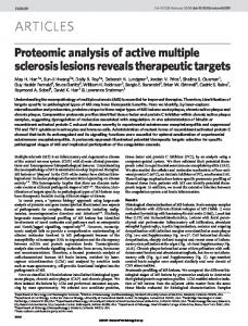
as well as new operations synchronized concurrence, exponentiation, product, and local product. The process operations of that paper are linearization, union, intersection, complement, star, augment closure, and prefix closure, whose definition we defer for now pending the appropriate integration of our framework with the current understanding of nondeterminism. We now illustrate and define three forms of sum: concurrence p|q, concatenation p;d q, and local concatenation p;d q. In these examples all edges are labeled with reals or ∞, with absence of an edge interpreted as distance −∞. These examples may be taken as pomset examples by ignoring the edge labels (equivalent to taking −∞ as 0 and everything else as 1), and as automata examples by treating distance d as the set of all strings of length at most d (making −∞ the empty language). In all of these forms of sum, the set of points of the sum is the disjoint union of those of p and q. That is, the basic step in forming the sum is to juxtapose p and q. Concurrence p|q is the least constrained form of sum. Labels on points, and distances within p and q, remain unchanged, while the distance from an event of p to one of q is −∞, and likewise from q to p. Disjoint concurrence differs from concurrence in that the labels from p and q are “marked” to distinguish them: the label a becomes a0 or a1 according to whether the point it labels is from p or q. c •
a 3 b
| • d
?
a c • = 3 ?• b d
Concurrence (a;3 b)|(c|d)
a
c •
a 5 -c @ = 3 @� ;2 3 5 R ? ?2 @ • b d b 2 d Concatenation (a;3 b);2 (c|d)
c •
a 3 ? B
;2
a 2 -c = 3
• D
? B2 D
Local Concat. (a;3 B);2 (c|D)
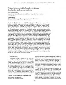
Figure 1. Additive Operations. Concatenation p;d q is like p|q, differing only with respect to the distances from p to q, which are the least possible distances no less than d. Disjoint concatenation is to concatenation as disjoint concurrence is to concurrence. Local concatenation p;d q is intermediate in strength between concurrence and concatenation: it only imposes the additional distance constraints of concatenation between colocated elements of p and q. For the above example we have identified location with case of label: lower case at one location, upper at the other. We now illustrate and define three forms of product, namely orthocurrence p ⊗ q, product p × q, and local product p×q.
a
c
ac
2 - ad
a
c
ac
2 - ad
a
c �B
ac 1- ae
@5 3 ⊗ 2 = 3 @ 3 R ? @ ? ? ? b d bc 2 bd
@2 3 × 2 = 3 @ 3 R ? @ ? ? ? d bc 2 bd b
3 × 2� B 1 = ? � BN B D e
Orthocurrence (a;3 b) ⊗ (c;2 d)
Product (a;3 b) × (c;2 d)
Local Prod. (a;3 b)×c(;2 D, ;1 c)
• BD
Figure 2. Multiplicative Operations. The underlying set of each of these products is the cartesian product of the underlying sets of their arguments (or a subset thereof in the case of local product), while their labels are corresponding tuples: thus if µ assigns labels to points then the label µ(hu, vi) in a product is hµp (u), µq (v)i. 5
Orthocurrence p|q is distinguished from other products by the distance from hu, vi to hu0 , v 0 i being d(u, u0 ) + d(v, v 0 ). Product p × q takes this distance to be min(d(u, u0 ), d(v, v 0 )). Local product p×q is obtained from product by deleting all points with mixed locations (again indicated by case in the example), and reducing the distance between tuples at distinct locations to −∞. For pomsets orthocurrence and product coincide, both combining the distances d(u, u0 ) and d(v, v 0 ) via conjunction. For automata they differ: orthocurrence uses concatenation, product intersection. Basic Constants. The empty schedule, denoted 0, has no events. It is the identity for all sums: concurrence, concatenation, and local concatenation. The unit schedule, denoted I, has one event with self-distance 0, and has the singleton alphabet {•}, whence that one event is labeled •. Up to isomorphism I is the identity for orthocurrence. The top schedule, denoted 1, differs from I in having self-distance ∞. Up to isomorphism it is the identity for product. (The isomorphism is not only between events but between labels, via the evident isomorphism between Σ and Σ × {•}.) We have illustrated these operations and constants for (dual) metric spaces, and indicated how to derive the corresponding pomset and automata examples. However these operations and constants also admit of obvious interpretations for the metrics themselves. Concurrence is respectively max, disjunction, and union for each of the ordered monoids consisting of truth values, reals, and languages, and is the same operation as concatenation and local concatenation. Orthocurrence is respectively arithmetic sum, conjunction, and concatenation. Product is respectively min, conjunction, and intersection, and is the same operation as local product.
3
Monoidal Categories and their Functors
Monoidal categories and enrichment are less well established in the computing literature than such other aspects of category theory as adjunctions. We therefore recall here enough details of these notions to make this paper self-contained at least on a first reading by those familiar with at least adjunctions. In addition our treatment will serve to define the perspective on these topics that we will assume of the reader, and to coordinate this perspective with the rest of the paper. Considerably more information on these topics can be found in the books of Mac Lane [Mac71] and Kelly [Kel82].
3.1
Monoidal Categories
Informally, a monoidal category amounts to a structure that is both a monoid and a category. Formally a strict monoidal category D = (D, ⊗, I) is a category D together with a functor ⊗: D2 → D called the tensor product 2 and an object I of D called the unit, such that the object part and the morphism part of D each form a monoid under ⊗ with respective identities I and 1I . We refer to (⊗, I) as a monoidal structure for the category D. The structure (Set, ×, {•}) with × cartesian product is not strict monoidal because in general X × (Y × Z) is not equal to (X × Y ) × Z, they are merely isomorphic. Moreover there is a particular isomorphism we would like to be able to assume is the one meant when we say that they are isomorphic, namely αXY Z : (X×Y )×Z → X × (Y × Z) defined as α(hhx, yi, zi) = hx, hy, zii. Similarly particular isomorphisms take the place of the two identity laws for the unit I = {•}. We therefore define a more general notion. A monoidal category D = (D, ⊗, I, α, λ, ρ) is as for strict monoidal 2 Mac
Lane writes ⊗ as 2.
6
categories but specifying natural isomorphisms α: (c ⊗ d) ⊗ e ∼ = c ⊗ (d ⊗ e), λ: I ⊗ d ∼ = d and ρ: d ⊗ I ∼ = d in place of the usual three-axiom basis for the theory of monoids. A symmetric monoidal category specifies an additional natural isomorphism γ: d ⊗ e ∼ = e ⊗ d. We shall confine ourselves to symmetric monoidal categories throughout, and understand “monoidal” to mean symmetric monoidal at all times. The intent of these isomorphisms is that they be canonical: if an element of one set corresponds to an element of another set at all, this is a universal or global correspondence. In particular there may be at most one such isomorphism between two sets, and in the case of a set in isomorphism with itself that isomorphism must be the identity. This intuition is formalized via certain coherence conditions, whose effect is that if there are multiple ways to infer by transitivity two isomorphisms between two sets, those isomorphisms must be the same. A strict monoidal category amounts to a monoidal category in which such isomorphisms are all identities. A monoidal category C is left closed (right closed) when − ⊗ b (a ⊗ −) has a right adjoint. When both exist it is called biclosed. When C is symmetric, either left closed or right closed implies biclosed, and in this case we simply call it closed. The right adjoint to − ⊗ b is notated −b : C → C and defined by an isomorphism Hom(a ⊗ b, c) and Hom(a, cb ) natural in a and c. Setting a to I yields via λ the natural isomorphism Hom(I,−) −− b→c∼ = I → cb , that is, Hom is naturally isomorphic to Hom0 : C op × C → C −→ Set. In this sense −− represents Hom(b, c), making it the internal hom(functor). As Rop ≥ in example (3) below shows, I need not determine ⊗ and hence the internal hom even up to isomorphism, showing that it is possible for the internal hom to contain information not present in the external hom even together with I. Since left adjoints preserve colimits, we have in any closed category (A + B) ⊗ C ∼ = A ⊗ C + B ⊗ C and C ⊗ (A + B) ∼ = C ⊗ A + C ⊗ B when the coproduct A + B exists and A ⊗ 0 ∼ =0∼ = 0 ⊗ A when the initial object 0 exists. A category D with all finite products determines the cartesian symmetric monoidal category (D, ×, 1). When the latter is closed (common but not universal, e.g. Top), D is said to be cartesian closed.
3.2
Examples of Monoidal Categories
We illustrate the above definitions with the monoidal categories we will be using in KL. Most of these will be closed and bicomplete, the kind we are most interested in. � (1) Each successor ordinal n+1, as an n+1-object category with n+2 morphisms i → j where 0 ≤ i ≤ j ≤ n, 2 forms the cartesian closed category algebraic topologists call [n]. That is, the symmetric monoidal structure is (n+1, ∧, n), and the right adjoint of ∧, the internal hom −− , must be the largest a such that a ∧ b ≤ c, namely n when b ≤ c and c otherwise. The product of two such cartesian closed ordinals or cco’s is the cco [m] × [n] = [m + n]. But the category n+1 = [n] admits other monoidal structures, all strict since n+1 has no nonidentity isomorphisms, and all bicomplete. Of these, 2n are idempotent (x ⊗ x = x), since each is representable as a permutation of {0, 1, . . . , n} whose domain partitions into two blocks on one of which the permutation is monotone and on the other antimonotone. Such a permutation can be written down by writing 0, 1, 2, . . . , I (the monotone block) from left to right and then reversing direction so as to write I + 1, I + 2, . . . , n (the antimonotone block) from right to left interleaved arbitrarily with the monotone block, leaving I at the far right. For n = 3 this can be done in eight ways, namely 0123, 013 2, 03 12, 032 1, 3 012, 3 02 1, 32 01, 321 0, here distinguishing the two blocks by writing the second as subscripts. Then x ⊗ y is taken to be the earlier of x and y in the permutation. Since
7
I is always at the right end of the permutation it will always be the identity of x ⊗ y. For ⊗ to be a functor it suffices that it be monotone, which the reader may verify. For n > 0 exactly half of these are closed. For to be closed we require that for any b and c there be a largest a for which a ⊗ b ≤ c. Setting c = 0 shows that 0 ⊗ b must be 0 for all b, whence a necessary condition is that the permutation start with 0. But this is also sufficient since there then exists a solution in a to a ⊗ b ≤ c, namely a = 0; finiteness then ensures a largest solution. These then are the idempotent closed ordinals or ico’s. There is therefore a unique ico 2, namely [1]. Here ⊗ is ∧ and I = 1. (The nonclosed one has ⊗ = ∨ and I = 0.) This category provides the metric for preordered sets. This two-valued cartesian closed logic is that of ordinary precedence, where for any pair u, v of events there are two cases: either u is constrained to precede v, or not. There are two closed categories on 3, each appearing implicitly in one of H. Gaifman’s two papers on concurrency. In each, the elements of 3 represent strengths of temporal precedence constraint between two events, with 0 representing no constraint. In the noncartesian case, call it 30 , 1 represents nonstrict temporal precedence and 2 strict, with 1 ⊗ 2 = 2 (u ≤ v < w → u < w). This structure is hidden in the two-relation “prosset” model [GP87] used in the proof of Kahn’s principle relative to a pomset-based semantics of nets [Pra86]. For the cartesian closed 3, 1 denotes “temporal” or accidental order and 2 causal [Gai89]. Here 1 ⊗ 2 = 1, that is, if u accidentally precedes v whereas v causes (necessarily precedes) w, then we may only infer that u accidentally precedes w. Thus one may identify the logic of causal and accidental precedence with the cartesian closed category 3. Of the four idempotent closed categories on 4, described by the first four permutations on the list five paragraphs above, the second and third have the same I, namely 2, but their internal homfunctors differ at 11 . Composing Hom(I, −) with either yields the external homfunctor for 4, whence the category and I together are not sufficient to determine either ⊗ or the internal homfunctor. However neither of these are cartesian closed, and in fact for all n the cartesian closed structure is the unique one with I = n. We do not as yet have a natural application for any of the structures on 4. (2) We have already discussed Set with ⊗ taken to be cartesian product, as a basic example of a nonstrict category. This monoidal structure for Set is cartesian closed, and will always be the one we have in mind when referring to Set as a monoidal category. In the case of Set the internal homfunctor is identified with its external one. (3) Let R∧ denote the real numbers together with ∞ and −∞ with the usual ordering and considered as a category in the usual way. Now R∧ is bicomplete, and furthermore is cartesian closed with a ⊗ b = a ∧ b, I = ∞, and internal homfunctor cb = ∞ for b ≤ c and c otherwise (cf. the cartesian closed ordinals above). op R∧ is isomorphic to its opposite Rop ∨ , the reals with their order reversed and with ⊗ now ∨. R∨ is the metric used for so-called ultrametric spaces. However a more useful closed structure for our purposes will be that obtained by taking tensor product to be not min but +, making the unit 0, and with ∞ + (−∞) = −∞, necessary in order to be closed. We denote it by R, or R+ when there might be confusion. To be closed requires cb satisfying a + b ≤ c ∼ = a ≤ cb , for which cb = c − b is the patently obvious solution. Hence R is bicomplete and closed, but of course not cartesian closed since, as we saw with the ordinals, a category admits at most one cartesian closed structure. We use R to represent lower bounds on delay. A distance of 5 units from event u to event v means that v must wait at least 5 units after u. Thus a delay of 0 from u to v simply asserts that v follows u, not necessarily strictly. 8
Now a delay of -5 units from u to v indicates that v may precede u by at most 5 units. Hence we can express upper bounds as negative lower bounds in the opposite direction. So to indicate that v must follow u by 2 to 5 units we bound from below the delay from u to v by 2 and that from v to u by -5. Combining these two directions, we may read the two oppositely oriented edges between u and v as together defining an interval. Here as with R∧ , R is isomorphic to its opposite Rop , the reals with their order reversed, however this time with the only change to the monoidal structure being ∞ + (−∞) = ∞, this being the one bit of asymmetry in R. As we have seen, Rop is the monoidal structure associated with ordinary metric spaces. A sometimes useful closed subcategory of Rop , namely Rop ≥ , is obtained by omitting the negative reals and −∞ [Law73]. The internal homfunctor then becomes truncated subtraction, in which negative differences are rounded up to 0. This is the category of generalized metric spaces; if the further restrictions are made that distances be symmetric and distinct points are a nonzero distance apart then we have the usual category of metric spaces and their contractions, modulo a detail about constant factors in the contractions. Rop ∨ may be similarly truncated and its I set to 0 to yield Lawvere’s basic example [Law73] of a cartesian and a noncartesian closed structure on the same category with the same I. (4) Take SR to be the category with objects arbitrary sets of reals and with morphisms X → Y just when X ⊆ Y . This poset is cartesian closed when we take ⊗ = ∩ and I = R. As with R however we shall prefer a different, hence noncartesian, closed structure, namely X ⊗ Y = {x + y | x ∈ X, y ∈ Y } with I = {0}, and with internal homfunctor Z Y = {x ∈ R | {x} + Y ⊆ Z}. The meaning of a set as a delay is that it consists of the disallowed actual delays. Thus ∅, like −∞ in R, is no constraint while R, like ∞, disallows all delays. We may now find R and Rop , as well as Rop truncated at 0, as subcategories of SR. We note in particular that R + ∅ = ∅, corresponding to ∞ + −∞ = −∞ in R. (5) Any monoid (M, ·, �) automatically forms a strict monoidal category by taking the set M as a discrete category. Alternatively M may be taken as indiscrete (the maximal preorder on M ). We refer to these as discrete and indiscrete monoids respectively. For a discrete monoid to be closed means simply that for all b, c, a + b = c has a solution in a, whence closed discrete monoids coincide with groups. No nontrivial discrete monoid has finite products or coproducts. An indiscrete monoid on the other hand is trivially closed with all limits and colimits. Only the fact that it is strictly monoidal saves it from total anarchy. A nonstrict monoidal codiscrete category is no more than an arbitrary binary operation on a pointed but otherwise indiscrete set; nevertheless all such are bicomplete and closed. (6) The category Pos of partially ordered sets forms a subcategory of the cartesian closed category Pros of preordered sets. The tensor product is direct or cardinal [Bir42] product of preorders. The cartesian closed structure of Pros is inherited from that of its underlying metric, namely the cartesian closed 2. The following section on enrichment treats the passage from the metric to the spaces in this example and the next two. By the same token Gaifman’s computations with distinct accidental and causal orders [Gai89] form a subcategory of a cartesian closed category of such computations with cycles allowed. As with Pros the cartesian closed structure is inherited from that of its underlying metric, here 3.
9
The Gaifman-Pratt “prossets” or preordered specification sets [GP87], each consisting of a set with an irreflexive partial order < and a preorder ≤, with u < v ≤ w → u < w, form a subcategory of a noncartesian closed category of “preprossets” in which < is itself just a preorder, but still meeting the condition u < v ≤ w → u < w.
3.3
Monoidal Functors
Monoidal functors, as the appropriate morphisms of monoidal categories, should preserve both the monoidal and category structure. Just as strict monoidal categories motivate monoidal categories, so do strict monoidal functors motivate monoidal functors. A strict monoidal functor F : D → D0 between monoidal categories D, D is a functor F : D → D0 between their underlying categories satisfying F x ⊗0 F y = F (x ⊗ y) and I 0 = F I for objects and similarly for morphisms. (The unit morphism is often written 1 instead of I or 1I .) Definition A lax monoidal functor (F, τ, t): (D, ⊗, I, α, λ, ρ, γ) → (D0 , ⊗0 , I 0 , α0 , λ0 , ρ0 , γ 0 ) consists of a functor F : D → D0 , a natural transformation τxy : F x ⊗0 F y → F (x ⊗ y), and a morphism t: I 0 → F I of D0 , with certain coherence conditions requiring that natural transformations constructed from τ and t commute with α, λ, ρ, γ and all the other natural transformations corresponding to the equations of the theory of commutative monoids [EK65]. When τ and t are both isomorphisms or both identities we call F respectively strong or strict. For the remainder of this paper the default will be strong, that is, we take “monoidal functor” to mean “strong monoidal functor.” In particular we take the morphisms of the category SMON of large (symmetric) monoidal categories to be the strong monoidal functors. We wish to be able to refer to the “points” of spaces. This is accomplished by the next definition. Definition. The category COSMON is the slice (comma) category SMON ↓ Set. Its objects are pairs (D, U ) called semiconcrete monoidal categories, where D is a (large) monoidal category and UD : D → Set is a monoidal “forgetful functor” for D. The morphisms F : (D, U ) → (D0 , U 0 ) of COSMON are monoidal functors satisfying U = U 0 F , τU = τU 0 τF , tU = tU 0 tF . Our interest in COSMON is that its members carry enough structure to support the definitions of the operations D! and D � E constructing categories of spaces and labeled spaces. While this adds some complexity to the development of enrichment, it does demonstrate the feasibility of adding such structure when needed. It would be particularly useful to have a characterization of what structures can be so added. All the examples of monoidal categories in our list above belong to COSMON; of these, only the discrete monoids are not bicomplete. Set, Pos, etc. are large objects in COSMON. The ordinal 1 is the null object of COSMON. Our insistence on the identity U = U 0 F , as opposed to just a natural transformation from U to U 0 F , makes for a clean division of labor between COSMON, where the kind language KL operates, and the objects of COSMON, where PSL operates. The significance of this identity is that, via functors of COSMON, KL may act on kinds without disturbing the underlying sets of objects of those kinds. For example when we replace a numeric metric by a Boolean one we identically preserve the vertex sets of the affected behaviors; only the distances between their elements change, from numbers to truth values. In PSL on the other hand we work in a fixed object D of COSMON, where we may do violence to vertex sets and alphabets via morphisms of D, but where we cannot change to another D and so have no control over the metric or the kind of alphabet.
10
As a pleasant fringe benefit the bidirectionality of the identity in U = U 0 F permits the domain of � to consist of all pairs F, G of functors of COSMON, not just those for which there exists a natural transformation from U 0 F to U . However this benefit would accrue even from a natural isomorphism h: U → U 0 F (assuming h commutes with both τ and t), whereas identity results in total separation of the domains of KL and PSL.
3.4
Examples of Monoidal Functors
(1) Consider functors F, G: R → 2, defined by F (x) = (x ≥ 0) and G(x) = (x > −∞). Each functor equips its target with an interpretation. F interprets u ≤ v as saying that u must precede v, while G makes it say that v can only precede u by a bounded amount. Only G however is strong monoidal, since F (1 + −1) = F (0) = 1 while F (−1) ∧ F (1) = 0. It is straightforward to show that G and the constantly true functors are the only strong monoidal functors from R to 2. In fact with the obvious order on the functors from R to 2 to make 2R a category, we have 2R ∼ = 2 in COSMON, with the constant functor in 2R corresponding to 1 in 2. Now consider any functor F from 2 to R. F must send 1 to 0, so F (0) cannot be positive. Moreover F (0) = F (0 ∧ 0) = F (0) + F (0) whence F (0) must be either −∞ or 0. Hence R2 ∼ = 2 (again with R2 made a category via the obvious order on its two functors), with the constant functor in R2 corresponding to 1 in 2. (2) The endofunctor x/2 from R to R that simply halves its argument is clearly monoidal. This is a “speedup” functor that allows one to pass to a world where everything happens twice as fast. In fact from F (a + b) = F (a) + F (b) and F (0) = 0 we infer that the linear speedups and slowdowns and their negations (time reversals) are the only functors, and thus we have RR ∼ = R. The ∞ and −∞ slowdowns are included, with the convention that 0 ⊗ ∞ = 0 = 0 ⊗ −∞. Their range in each case is isomorphic to the noncartesian closed ordinal 30 with the convention that ∞/∞ = ∞, −∞/∞ = −∞, ∞/n = 0 for all other n ∈ R and likewise for the / − ∞ speedup. (3) We leave it to the reader to verify that 22 ∼ = 2 with the constant functor corresponding to 1 as always.
4
Enriched Categories and the ! Operator
We now introduce the basic notions of enriched categories. Our hope is that these will be made more accessible via definitions that are not only close at hand but presented from the same perspective as the applications. Enriched categories or V -categories are treated briefly by Arbib and Manes [AM75] and exhaustively and precisely by Kelly [Kel82]. Section I-8 of Mac Lane also touches on them, without calling them such. As far as we are aware ours is the first proposed engineering application of Lawvere’s vision [Law73] of enriched categories as a combined generalized metric and logic.
4.1
D-categories
The essence of an enriched category may be found in an ordinary category C. Write δ(u, v) for the set of morphisms from u to v. Associated with each triple u, v, w of objects of C is a function muvw : δ(u, v) × δ(v, w) → δ(u, w) defining composition. And to each object u there is a function ju : {·} → δ(u, u) picking out the identity element 1u ∈ δ(u, u).
11
We pass from this account of an ordinary category C to the notion of a category C enriched in D, or Dcategory, by requiring each δ(u, v) to be an object of D instead of a set, and each muvw and ju be a morphism of D instead of a function. The class of objects of C do not participate in this passage: the objects of C remain a class. A functor F : A → B participates partially in this passage: when we view it as the D-functor F : A → B, its object part remains unchanged but its action on morphisms, viewed for each pair uv of objects of A as a function Fuv : δ A (u, v) → δ B (F (u), F (v)), becomes a morphism of D between homobjects δ A (u, v) and δ B (F (u), F (v)) of A, B respectively. From this viewpoint, ordinary categories and functors between them are Set-categories and Set-functors, that is, categories and functors enriched in Set. Definition. A D-category A = (V, δ, m, j), or category enriched in D, consists of a set V , a function δ: V 2 → ob(D), and families of morphisms of D, namely compositions muvw : δ(u, v) ⊗ δ(v, w) → δ(u, w) and identities ju : I → δ(u, u), such that for all objects u, v, w in V the following diagrams commute. These diagrams express associativity of composition, and the left and right identity laws, explained below.
For D = 2 the diagrams expressing the associativity and identity laws hold vacuously since D is an ordered set. Thus composition and identity become muvw : u ≤ v ∧ v ≤ w → u ≤ w ju : u ≤ u expressing respectively transitivity and reflexivity. Thus 2-categories (categories enriched in 2, as opposed to 2-categories which here are Cat-categories) are just preorders. For D = Rop , also an ordered set, we again may ignore the associativity and identity laws. Here we get muvw : d(u, v) + d(v, w) ≥ d(u, w) ju : 0 ≥ d(u, u)
For D = Cat we obtain ordinary 2-categories, along the same lines as for D = Set but with the addition of 2-cells between morphisms of the same homset.
4.2
D-functors
Definition. A D-functor F : A → B where A and B are D-categories consists of a function F : VA → VB between object sets together with a family Fuv : δA (u, v) → δB (F u, F v) of morphisms between homobjects satisfying the following conditions stating that compositions and identities are preserved.
The elements of a D-functor are depicted on the left of the following figure, and compose in the obvious way as shown on the right.
12
u δA (u, v) u ============⇒ v F
Fuv ∨
∨
δA (u, v) ===============⇒
F
Fuv
v F
∨ ∨ ∨ δB (F u, F v) F u ===============⇒ F v
F ∨
G ∨
GF u,F v ∨
G ∨
It can be seen that 2-functors are monotone functions, R-functors and Rop -functors are expanding and contracting maps respectively, and Set-functors are ordinary functors. In our computational application a D-functor is an event map which maintains all temporal constraints, though the result may have more constraints than the source.
4.3
Enrichment as a Function
We now define the object part of the functor −!: COSMON → COSMON. Given a semiconcrete monoidal D define D! to be the category D-Cat of small categories enriched in D. D! is symmetric monoidal as follows [EK65]. The tensor product of two D-categories A and B is defined to have as objects the cartesian product VA × VB , and homobjects δ((u, v), (u0 , v 0 )) = δA (u, u0 ) ⊗D δB (v, v 0 ). The symmetry of D ensures that appropriate composition morphisms can be defined and that D! is symmetric to boot. The corresponding unit I is the one-object category with homobject δI (·, ·) = ID . To make D! semiconcrete we define the forgetful functor UD! : D! → Set mapping each D-category A to its underlying set VA of objects and each D-functor to its object map. UD! is monoidal by the above definition of ⊗ for D!. In our application U yields the event set U (b) of a behavior b. We summarize the above as follows.
Lemma 1 If D is an object of COSMON then so is D!.
4.4
Enrichment as a Functor
We now define the action of ! on morphisms of COSMON. Definition Given a monoidal functor (F, τ, t): D → E, define the functor (F, τ, t)! = (F !, τ !, t!): D! → E! as follows:
13
F ! takes a D-category A to the E-category F !A = (V, δ, m, j) defined by V = VA (that is, UD! = UD0 ! F !) δ(u, v) = F (δA (u, v)) muvw = F (mA uvw )τδA (u,v)δA (v,w) ju = F (juA )t F ! takes a D-functor G: A → B, to that E-functor F !G which has the same object function and takes (F !G)uv to F (Guv ). Thus F ! acts only on the distances within a behavior, and on the “distance comparison” part of a morphism of behaviors. For D-categories A and B and objects u and u0 or A, and v and v 0 of B, define (τ !)(u,v)(u0 ,v0 ) = τδA (u,u0 ),δB (v,v0 ) . By the definition of F !, F !ID! is an E-category with a single object. Thus there is a unique possible object map for t!: IE ! → F !ID! . t! on homobjects must be a map from IE → F ID ; define this map to be t. Lemma 2 If (F, τ, t): D → E is a morphism of COSMON then so is (F !, τ !, t!): D! → E!.
We omit the straightforward, though tedious, proof. Finally, by checking that ! preserves composition and identities, we obtain the following.
Theorem 3 ! is an endofunctor on COSMON.
4.5
Examples
(1) Section 2 contains a figure illustrating the example (a;3 b) ⊗ (c;2 d) of orthocurrence. The triangle inequality requires the upper bounds on diagonals across squares and rectangles to be at most the sum of the bounds encountered along any path around the sides, e.g. 5 from ac to bd. This is exactly the effect obtained by defining tensor product of spaces (enriched categories) in terms of the addition (tensor product) of the underlying metric. Had we defined tensor product of spaces in terms of ordinary product in the metric (min), we obtain the next example, ordinary product of spaces. (2) Consider the monoidal functor F : R → 2 which takes −∞ to 0 and all else to 1. Application of F ! to each of the illustrated examples of Section 2 with vertex labels deleted to make them objects of R!, produces the corresponding object of 2!, a poset, in effect by erasing the edge labels.
4.6
Continuity of !
We now show that ! enjoys certain continuity properties. These will be used in section 7 to show that all KL kinds are bicomplete and closed, which in turn ensures that PSL is well-defined. Proposition 4 If D has an initial object 0 and a natural isomorphism A ⊗ 0 ∼ = 0 then D! has coproducts. 14
The natural isomorphism A ⊗ 0 ∼ = 0 always exists when D is closed. A discrete category is a copower in Cat of 1, that is, the coproduct of a set of one-object categories, yielding the following similar result: Proposition 5 If D has an initial object 0 and 0 ⊗ A ∼ = A ⊗ 0, then the forgetful functor UD! : D! → Set =0∼ has a left adjoint D: Set → D! taking a set S to the corresponding discrete D-category (δDS (u, v) = I if u = v, 0 otherwise). The dual result to this, though not with a dual proof, is: Proposition 6 If D has a final object 1, UD! : D! → Set has a right adjoint E: Set → D! taking the set X to the corresponding chaotic (codiscrete) D-category (δDS (u, v) = 1 for all u, v). Meanwhile, for the case of general colimits we refer to a result of [BCSW83]. Theorem 7 If D is cocomplete and D is closed then D! is cocomplete. There is also a similar but much easier result about limits. PSL needs limits for local product and hence local concatenation. Theorem 8 If D has limits of (small) type J, then so does D!. If any one theorem could be considered at the heart of enriched categories it is the following. Kelly’s proof ([Kel82] p.55, see also Lawvere [Law73] p.153) is dauntingly formal, to which we offer an informal counterpart. Theorem 9 If D is complete and closed then D! is closed.
Proof: The objects of the D-category C B are of course just the D-functors from B to C. What is less obvious is the appropriate homobject δC B (U, V ) abstracting the homset of natural transformations between Q any two D-functors U,RV of C B . The natural and unnatural transformations are given by b∈B δC (U b, V b); we seek its subobject b∈B δC (U b, V b) (an end [Mac71] p.219) consisting of just the natural ones. Now for D = Set such a transformation τ determines, for all b, b0 , two functions ρτ , στ : δB (b, b0 ) → δC (U b, V b0 ), 0 that is, two elements of δC (U b, V b0 )δB (b,b ) . Here ρτ takes f : b → b0 to V (f ) ◦ τb , while στ takes the same f to τb0 ◦ U (f ). But these are just the two sides of the square
which must be equal for τ to be natural. Encapsulating “for all b, b0 ” as a product over b, b0 ∈ B and generalizing to arbitrary D (formalized in Kelly’s proof), we may therefore obtain the desired homobject δC B (U, V ) as the equalizer of Y Y 0 δC B (U, V ) δC (U b, V b) δC (U b, V b0 )δB (b,b ) . b,b0 ∈B
b∈B
15
This construction required an exponential, two products, and an equalizer, for which it suffices that D be complete and closed.
5
Comma Categories and the � Operator
Given a space p and a labeling set or alphabet Σ, we label the underlying set U (p) of points of p with a function µ: U (p) → Σ. For p a poset this is the notion of pomset or partially ordered multiset as a labeled partial order. Our framework can be simplified by dropping the assumption that Σ is set and instead associating with the category supplying Σ a functor V that somehow interprets Σ as a set. Our labeling function then becomes µ: U (p) → V (Σ). But this is what it means to be an object of the comma category (U ↓V ). Moreover the morphisms of this comma category from µ: U (p) → V (Σ) to µ0 : U (p0 ) → V (Σ0 ), namely pairs of maps f : p → p0 and t: Σ → Σ0 such that V (t)µ = µ0 U (f ), turn out to be just what we need.
5.1
The Function �
Given categories D, E in COSMON (i.e., both symmetric monoidal equipped with monoidal functors (U, τU , tU ): D → Set, (V, τV , tV ): E → Set, respectively), we define D � E to be the comma category U ↓ V . Recall that this is the category whose objects are triples hx, µ, ui where µ: U x → V u, and whose morphisms are pairs hf, gi such that the following square commutes:
D � E can be made symmetric monoidal by defining the tensor product
⊗ to be the outer square of
The unit object of D � E is taken to be ID � E = hID , h, IE i, where h = tV t−1 U
(In fact one may use these definitions for ⊗ and I in the case where V is only lax monoidal; U must still be strong monoidal). Now we must show that this product is associative and symmetric, and has I for its identity. We treat only associativity, the other natural transformations being treated similarly. Recall that associativity in a monoidal category D is a natural isomorphism αzz0 z00 mapping the functor (z ⊗ z 0 ) ⊗ z 00 : D3 → D to the functor z ⊗ (z 0 ⊗ z 00 ): D3 → D. 16
Take αµµ0 µ00 in D�E, where µ: x → y, µ0 : x0 → y 0 , µ00 : x00 → y 00 , to be the pair hαxx0 x00 , αyy0 y00 i of associativity transformations in respectively D and E. This is a well-defined morphism because V (α)(µ⊗(µ0 ⊗µ00 )) is equal to ((µ ⊗ µ0 ) ⊗ µ00 )U (α), using properties of monoidal functors and natural transformations. The coherence conditions on αD � E are established similarly. We complete the definition of the object D � E by defining its underlying set, via the following functor to Set. We shall derive the properties of this functor that we shall need at the end of this section.
5.2
� as a Functor
To complete the description of the functor � we describe its action on morphisms (i.e., functors) F, G of COSMON. Recall that we impose the condition U = U 0 F in the definition of the morphisms F of COSMON as well as the condition that F be strong monoidal. The functor F � G: COSMON 2 → COSMON acts thus: >� where π0 projects onto D as before and F � G takes each morphism hf, gi of D � E to hF f, Ggi = hU 0 F f, V 0 Ggi.
We now need to verify that F � G is strong monoidal. This involves exhibiting a morphism τF � G : (F � G)hx, µ, ui⊗ (F � G)hy, ν, vi → (F � G)(hx, µ, ui⊗hy, ν, vi) of D0 � E 0 for any pair hx, µ, ui, hy, ν, vi both in D � E, namely that given by pairing τF : F x × F y → F (x ⊗ y) with the corresponding τG . That this is indeed a morphism of D0 � E 0 depends on the commutativity of the squares appearing in
which follows from the τU = (U 0 τF )τU 0 condition in the definition of COSMON. That the morphisms τF � G constitute a natural transformation and that they satisfy the appropriate coherence conditions directly follows from the corresponding naturality and coherence conditions on τF and τG .
5.3
Continuity of �
We now wish to lift limits and colimits that exist in the component categories to comma categories defined from them. To do this we must deal with functors into comma categories. The following lemma can be applied whenever functors into a comma category are to be defined. It states that defining a functor from a category J into (U ↓V ), where U : A → C and V : B → C, is essentially equivalent to defining functors F : J → A and G: J → B and a natural transformation from U F to V G. Furthermore, natural transformations between such functors are essentially equivalent to a pair of natural transformations satisfying a certain commutativity condition. For any functor F : X → Y denote by F J the functor from the functor category X J to Y J defined by “left-composition with F ”. Then we have: Lemma 10 (U ↓ V )J ∼ = (U J ↓ V J ). 17
Outline of Proof: The comma category U ↓ V has the projections π0 : U ↓ V → A and π1 : U ↓ V → B, and defines a natural transformation ν: U π0 → V π1 . (In fact this is an alternative definition of the concept of a comma category.) Hence, given a functor, F : J → U ↓ V , we can define functors π0 F : J → A and π1 F : J → B, and a natural transformation ν ◦ F : U π0 F → V π1 F . This defines an object of the comma category (U J ↓ V J ). It is routine to extend this mapping to a functor (U ↓ V )J → (U J ↓ V J ) and show that it is an isomorphism of categories.
From this lemma we may obtain the following very useful theorem. Tarlecki [Tar85] proves the weaker version of this theorem in which J is not a parameter of the theorem, in that A and B are required to have all limits rather than just J-limits. The lemma in Mac Lane’s treatment of Freyd’s Adjoint Functor Theorem [Mac71, V.6]) treats only the case A = 1 of Tarlecki’s theorem.
Theorem 11 Let U : A → C and V : B → C be functors, and J be a category. If A and B have all J-limits and V preserves J-limits then the comma category (U ↓ V ) has all J-limits
Proof: Let F : J → (U ↓ V ) be an J-diagram in (U ↓ V ). Then by lemma 10, F can be considered as a triple, hF1 , µ, F2 i where F1 : J → A F2 : J → B µ: U F1 → V F2 Since A and B have J-limits, both F1 and F2 have limits. Denote their limiting cones by λ1 : lim F1 → F1 and λ2 : lim F2 → F2 respectively. Since V preserves J-limits, V (lim F2 ) is a limit of V F2 , with limiting cone V λ2 . Now the composite natural transformation U (lim F1 ) → U λ1 U F1 → µV F2 is a cone from U (lim F1 ) to V F2 , so by the universal property of limits there exists a unique arrow p such that the following diagram of functors and natural transformations commutes. (Note: in this and the following diagrams an object of C represents the constant functor to that object and an arrow of C represents the “constant” natural tranformation between such constant functors.)
U (lim F1 )
U λ1
p
? V (lim F2 )
- U F1 µ
V λ2
? - V F2
Now we claim that hlim F1 , p, lim F2 i is the limit of F , and that the limiting cone is defined by the pair of natural transformations hλ1 , λ2 i.
18
For suppose we have an object, hA, f, Bi and a cone κ: hA, f, Bi → F . κ can be considered as a pair of natural transformations, κ1 : A → F1 and κ2 : B → F2 . Since F1 and F2 have limits there must exist unique maps a: A → lim F1 and b: B → lim F2 which factor κ1 and κ2 through λ1 and λ2 respectively. Consider the following diagram of natural transformations.
f
UA
- VB
A
U κ1
A Ua AU U (lim F1 ) � � U λ1 �� ?�
U F1
� � �� V (lim F2 ) V κ2 A A V λ2 AAU ? -V F2 Vb
p
-
µ
The outer square of this diagram commutes because κ is an arrow in the comma category. The two inner triangles commute by definition of a and b. The lower inner square commutes by definition of p. Now we wish to show that the upper inner square commutes. We do this by showing that the cone (V λ2 ).(V b).f is identical to the cone (V λ2 ).p.(U a). Since there must be a unique arrow which factors this cone through the limiting cone V λ2 , we can conclude that the arrows (V b).f and p.(U a) must be identical. This is the required commutativity condition. But we have (V λ2 ).(V b).f
= (V κ2 ).f = µ.(U κ1 ) = µ.(U λ1 ).(U a) = (V λ2 ).p.(U a)
definition of b outer square commutes definition of a lower square commutes
This proves the required commutativity, which shows that ha, bi is an arrow in U ↓ V and that it factors κ. That ha, bi is the unique such arrow follows from the fact that a must factor κ1 through the limiting cone λ1 , so a is the unique such arrow. Similarly, b must factor κ2 through λ2 , and so is unique. Note that the proof gives an explicit construction of limits in a comma category when the conditions of the theorem are satisfied. The same technique allows us to construct colimits:
Corollary 12 If A and B have all J-colimits and U preserves J-colimits then U ↓ V has all J-colimits.
Proof:
For any functor U : A → C, let U op be the corresponding functor U op : Aop → C op . Observe that (U ↓ V )op = (V op ↓U op ).
With rather more work we may show that under appropriate conditions U ↓ V is closed. 19
Theorem 13 Suppose that A and B are monoidal closed, and that C is monoidal. Suppose further that F : A → C is a strong monoidal functor, that G: B → C is (lax) monoidal, and that A has all pullbacks. If F admits a right adjoint, R, then F ↓ G is closed.
Proof Outline: The proof is in three stages. Under the assumptions of the theorem we show: 1. R is monoidal and hence that RG is monoidal; 2. F ↓ G is isomorphic to 1A ↓ RG; and finally 3. For any monoidal functor H: A → B, 1A ↓ H is closed.
We adopt the following notation. Suppose that F has right adjoint R. For any arrow g: F A → B denote the adjoint transpose by g ] : A → RB. Dually, denote the adjoint transpose of f : A → RB by f [ : F A → B. Observe that for appropriate arrows f, g and g 0 we have (g 0 g)] �] g(F f ) The dual results, (f f 0 )[ = (f [ )(F f 0 ) and (Rg 0 )f
�[
= (Rg 0 )g ] = g ] f. = g 0 f [ will also be useful.
We now proceed with the proofs of the three lemmas which prove the theorem.
Lemma 14 Let F : A → C be strong monoidal and have a right adjoint, R. Then R is monoidal.
Proof:
b I → F I be the isomorphisms which make F monoidal. Let φ: F A ⊗ F B → F (A ⊗ B) and φ:
Define ψ: RX ⊗ RY → R(X ⊗ Y ) to be the adjoint transpose of the composite φ−1
�⊗�
F (RX ⊗ RY ) −→ F RX ⊗ F RY −→ X ⊗ Y ; b I → RI to be (φb−1 )] . and ψ: To show that φ and φb make R into a monoidal functor, we must show that they satisfy the coherence conditions. We give here the proof of the associativity condition. The proofs of the other two conditions are similar. F is monoidal, so we know that the following commutes:
(F RX ⊗ F RY ) ⊗ F RZ
φ⊗1 - F (RX ⊗ RY ) ⊗ F RZ
φ - F (RX ⊗ RY ) ⊗ RZ �
α ? F RX ⊗ (F RY ⊗ F RZ)
Fα 1⊗φ - F RX ⊗ F (RY ⊗ RZ) 20
φ
? - F RX ⊗ (RY ⊗ RZ)�
Rearrange to obtain the equation α(φ−1 ⊗ 1)φ−1 = (1 ⊗ φ−1 )φ−1 F α. Compose both sides of the equation with � ⊗ (� ⊗ �). Then the left hand side of the new equation is: � � ⊗ (� ⊗ �) α(φ−1 ⊗ 1)φ−1 = = = =
α(ψ [ ⊗ �)φ−1 α((�(F ψ)) ⊗ �)φ−1 α(� ⊗ �)φ−1 F (ψ ⊗ 1) αψ [ F (ψ ⊗ 1)
The right side of the new equation is � � ⊗ (� ⊗ �) (1 ⊗ φ−1 )φ−1 (F α) = (� ⊗ ψ [ )φ−1 (F α) �� = � ⊗ �(F ψ) φ−1 (F α) = (� ⊗ �)φ−1 F (1 ⊗ ψ)(F α) = ψ [ F (1 ⊗ ψ)(F α)
Apply ] to both sides of the new equation and simplify using the properties of ] to obtain the required condition (Rα)ψ(ψ ⊗ 1) = ψ(1 ⊗ ψ)α.
Lemma 15 Let R: C → A be a right adjoint of F , considered as a monoidal functor as described in the previous lemma. Under the conditions of the theorem F ↓ G and 1A ↓ RG are isomorphic monoidal categories.
f]
f
Proof: To each object F A −→ GB associate the corresponding object A −→ RGB. It is straightforward to show that this correspondence can be extended to an isomorphism of categories. Now we show that the tensor product of the two categories coincide. Let γ be the natural transformation GB1 ⊗ GB2 → G(B1 ⊗ B2 ). Let φ be the natural isomorphism F A1 ⊗ F A2 → F (A1 ⊗ A2 ). Denote the corresponding transformation for R by ψ, recalling that ψ = ((� ⊗ �)φ−1 )] . Hence, the transformation for the composite functor RG is (Rγ)ψ. f1
f2
Consider two objects, F A1 −→ GB1 and F A2 −→ GB2 . Applying ] and then taking the tensor product in 1 ↓ RG results in the composite arrow f ] ⊗f ]
(Rγ)ψ
1 2 A1 ⊗ A2 −→ RGB1 ⊗ RGB2 −→ RG(B1 ⊗ B2 ).
We want to show that this arrow is identical to the result of first taking tensor product in F ↓ G and then applying ], namely (γ(f1 ⊗ f2 )φ−1 )] .
21
But we have
(Rγ)ψ(f1] ⊗ f2] ) = (Rγ)((� ⊗ �)φ−1 )] (f1] ⊗ f2] ) �] = γ(� ⊗ �)φ−1 F (f1] ⊗ f2] ) �] = γ(� ⊗ �)(F (f1] ) ⊗ F (f2] ))φ−1 �] = γ(�F (f1] ) ⊗ �F (f2] ))φ−1 � ] = γ(f1 ⊗ f2 )φ−1 ,
definition of ψ properties of ] φ is natural
as required.
Lemma 16 Let A and B be closed monoidal categories, and H: A → B be a monoidal functor. Suppose that A has pullbacks. Then the monoidal category 1A ↓ H is closed.
Proof:
Denote the natural transformation HB1 ⊗ HB2 → H(B1 ⊗ B2 ) by γ.
Let hA1 , f1 , B1 i and hA2 , f2 , B2 i be two objects of 1 ↓ H. We show that tensor product has a right adjoint by constructing an object universal from the functor hA1 , f1 , B1 i ⊗ − to hA2 , f2 , B2 i. Consider the pullback
π2 - H[B1 , B2 ]
X
((H�)γ)] ? [HB1 , HB2 ]
π1
? [A1 , A2 ]
[f1 , 1] ? [A1 , HB2 ]
[1, f2 ]
We will show that the top line of this diagram is the required universal object. Firstly, we claim that the universal arrow to hA2 , f2 , B2 i is given by
A1 ⊗ X
f1 ⊗ π2 - HB1 ⊗ H[B1 , B2 ]
π1[
γ - H(B1 ⊗ [B1 , B2 ]) H�
? A2
f2
? -HB2
To see that this square commutes, apply [ to both directions around the pullback square. It is immediate that ([1, f2 ]π1 )[ equals (f2 π1[ ). For the other direction, observe from standard properties of adjunctions that [f1 , 1] = (�(f1 ⊗ 1))] . Hence, [f1 , 1]((H�)γ)] π2
�[
22
= [f1 , 1][ (1 ⊗ ((H�)γ)] )(1 ⊗ π2 ) = �(1 ⊗ ((H�)γ)] )(f1 ⊗ π2 ) = (H�)γ(f1 ⊗ π2 ), as required. Suppose now that there exists a commuting square f1 ⊗ g - HB1 ⊗ HC
A1 ⊗ Y
γ - H(B1 ⊗ C)
p
Hq ? A2
? - HB2
f2
� B is closed, so q can be factored into �(1 ⊗ q ] ). By the naturality of γ, H(1 ⊗ q ] ) γ is equal to γ(1 ⊗ Hq ] ), so we obtain � f2 p = (H�)γ f1 ⊗ (Hq ] )g . Applying ] to both sides of this equation shows that the following square commutes.
g Y
- HC
H(q ] ) - H[B1 , B2 ] (f1 ⊗ 1)] ? [A1 , HB1 ⊗ H[B1 , B2 ]
p]
? [A1 , A2 ]
[1, (H�)γ] ? [A1 , HB2 ]
[1, f2 ]
Consider the right side of this square. Observe that [1, (H�)γ](f1 ⊗ 1)] = ((H�)γ(f1 ⊗ 1))] . Now consider the right side of the pullback square that defines X. [f1 , 1]((H�)γ)]
= = = =
(�(f1 ⊗ 1))] ((H�)γ)] (�(f1 ⊗ 1)(1 ⊗ ((H�)γ)] ))] (�(1 ⊗ ((H�)γ)] )(f1 ⊗ 1))] ((H�)γ(f1 ⊗ 1))]
So we know that the right arrow of this square is the same as the right arrow of the pullback square defining X. But then there must exist a unique map r: Y → X such that π2 s = (Gq ] )g and π1 s = p] . The first equation is precisely the condition that hs, q ] i be a well-defined map from hY, g, Ci to hX, π2 , [B1 , B2 ]i. The second shows that hs, q ] i factors the original map hp, qi through the counit of the adjunction. Uniqueness follows from the unique factorization of q through � and properties of pullbacks. Our original application of the D � E construct was to partially ordered multisets or pomsets. A pomset p = hP, µ, Σi is just a poset P , labeled by a function µ: V (P ) → Σ for some set Σ, where V (P ) is the set of 23
vertices or points of P . This makes it an object of Pom = Pos � Set (following the convention whereby the identity functor 1Set is contracted to Set in this context). A morphism of pomsets f : hP, µ, Σi → hP 0 , µ0 , Σ0 i consists of a monotone event map f : P → P 0 on the underlying posets together with an alphabet map or translation t: Σ → Σ0 from Σ to Σ0 , such that tµ = µ0 f (i.e., the event map and translation are consistent with respect to the labelings). We can view Pom as the full subcategory of Prom = 2! � Set, the latter generalizing the notion of pomsets by allowing P to be a preorder.
5.4
The Forgetful Functor for D � E
We have already defined the forgetful functor U : D � E → Set as
This makes the underlying sets of objects of D � E those of objects of D. If the objects of D are spaces while those of D � E are labeled spaces, the underlying sets of the latter are the same as those of the former, i.e. the labels are ignored. We now give conditions under which this forgetful functor has a left adjoint. We have no information on right adjoints.
Lemma 17 Let F : A → C and G: B → C be functors having left adjoints F 0 and G0 , respectively. Suppose further that F F 0 is the identity functor on A (so that C can be seen as a coreflective subcategory of A.) Then π the projection functor (F ↓ G) −→ A has a left adjoint.
Proof: Let η G : C → GG0 C be the unit of the adjunction G0 a G. I claim that the “free (F ↓ G) object on an object C” can be defined by ηG
F F 0 C = C −→ GG0 C, and the unit of this adjunction is the unit of the adjunction F 0 a F , denoted η F : C → F F 0 C = πhF 0 C, η G , G0 Ci.3 For suppose that p: C → πhA, f, Bi is an arrow of C. By definition of π, the codomain of p is F A, hence p corresponds to an arrow p[
F 0 C −→ A. The adjunction G0 a G then ensures the existence of a unique q making the following diagram commute
C
ηF - F F 0C S p S S w S
ηG
F p[ ? FA
- GG0 C . . . Gq . . ? - GB
f 3F F 0C
= C but it is not necessary that η F be the identity arrow of C, although it is always an automorphism.
24
Thus hp[ , qi is an arrow factoring p. Properties of the two adjunctions ensure that it is the unique such arrow. This completes the proof.
Corollary 18 Let D and E be objects of COSMON, and suppose that D has an initial object 0 preserved by tensor product with any object. Let UE have a left adjoint. Then the forgetful functor from D! � E also has a left adjoint.
Proof: By proposition 5 UD! has a left adjoint D taking any set X to the discrete category DX. Note that π UD! DX = X. So the lemma applies, and the projection D � E −→ D has a left adjoint. By composition with D we obtain a left adjoint to UD�E .
6
Abstract Specification of the Operations
Having established the categorical framework for our abstract treatment of time, we now define the operations of our algebras of behaviors. The sense in which time is abstract is that a fixed category D of spaces is assumed to be given as a parameter. The definitions may therefore refer to D, but will not assume that D has any a priori structure such as labels on points or a metric between points. Each choice of D determines an algebra of behaviors, really a class of behaviors since we impose no cardinality bounds on the number of events in a behavior, other than the requirement that the events of a behavior form a set. Most operations are of arity a small integer. On occasion however, e.g. when certain arguments are required to have the same domain or the same codomain, the arity will be a graph, meaning that the arguments will be organized as a functor from that graph. For example if the arity is the 3-vertex 2-edge graph of shape < (two edges pointing to the right) then the arguments are two morphisms with a common domain. This is made uniform by regarding each integer arity n as a discrete (edge-less) graph with vertices 1 through n. Disjoint Concurrence, dconcur(p, q), notation p + q. The disjoint concurrence of behaviors p and q performs both p and q concurrently, that is, unconstrained in time. It is defined as the coproduct p + q in D. Disjoint Concatenation, dconcat(p, d, q), notation p;d q. The disjoint concatenation of behaviors p and q with delay d performs both p and q as in disjoint concurrence, but in the order p, then a delay d: I + I → d0 , then q. It is defined by the pushout where the top morphism is the sum πp + πq : p × q + p × q → p + q of the two projections πp : p × q → p and πq : p × q → q from p × q, and (I + I) ⊗ r ∼ =I ⊗r+I ⊗r ∼ = r + r. Concurrence, concur(p → k ← q), notation p||k q, or p||q when k is supplied by context. The concurrence of behaviors p and q over k performs both p and q concurrently, coordinated by k. It is defined as the coproduct of the morphisms p → k and q → k in D/k, the comma or slice category of morphisms to k (“objects over” k), itself a morphism to k and thus retaining the coordination. Concatenation, concat((p, d, q) → k), notation p;dk q. The concatenation of p with q performs both p and q concurrently, coordinated by k, but in the order p, then a delay d, then q. It is defined as for disjoint concatenation, with the pushout formed in D/k. Local disjoint concatenation, ldconcat(d, p → L ← q), notation p;dL q. The local disjoint concatenation of behaviors p and q with delay d performs p and q concurrently except that events of p at a given location 25
must be followed by a delay d: (I + I) → d0 before performing events of q at that location. It is defined analogously to disjoint concatenation via the pushout
where L= : p ×L q → p × q is the standard embedding, namely the equalizer Lp ◦ πp and Lq ◦ πq , and the rest is as for disjoint concatenation. Local concatenation, p;dkL q, is the appropriate combination of concatenation and local disjoint concatenation. Orthocurrence, orthocur(p, q), notation p ⊗ q. The orthocurrence of behaviors p and q consists of the flow of p and q past each other. It is defined as their tensor product p ⊗ q. Unit, unit, notation I. The unit is a one-event behavior that flows by unnoticed. It is defined as the unit I of D, being the unit for orthocurrence. Observation, observe(q, r), notation rq . The observation of behavior q by behavior r is the result of observing every stage of every event of q, where the stages of an event of q are defined as the events of r. It is defined by the adjunction p ⊗ q → r ∼ = p → rq , that is, −q is right adjoint to − ⊗ q. Product, product(p, q), notation p × q. The product of behaviors p and q consists of all pairs (a, b) of constituents a of p and b of q, with all the structure of p and q preserved coordinatewise. It is defined as their ordinary (categorical) product p × q. Local product, lproduct(p → L ← q), notation p ×L q. The local product of behaviors p and q consists of all pairs (a, b) such that a and b are L-colocated (conceptually, at the same location l ∈ L). It is defined as the pullback
7
The Kind Language KL
The kind language KL consists of terms naming certain kinds in COSMON. KL terms are among those terms that can be built up from ground terms 1, 2, 3, 30 , R, Rop , and SR using the operations ! and �. We make each ground kind semiconcrete by taking its underlying set functor U to be the constant functor yielding a singleton. Some terms in this language are neither useful nor well-behaved, for example 2�1!, which denotes a category that is not closed. In forming D � E we shall restrict D to terms built using ! and �. That is, we forbid D to be a ground term, as in 2 � 2. In addition, in forming E 0 � E we shall restrict E to terms of the form D! and ground terms. That is, we forbid E to be built using �. The reasons for these restrictions have to do with which adjoints the various forgetful functors have. The forgetful functor we defined for ground types two paragraphs back has a left adjoint, namely the constant functor yielding the initial object. However it cannot have a right adjoint since it does not preserve the initial object. While we could easily fix this by redefining U (0), we could not as easily fix the fact that U must map I to a singleton (being monoidal) but I + I to a doubleton if U has a right adjoint, impossible since I + I = I in all our ground types. Moreover the forgetful functor we defined for D � E has a right adjoint, but we have no guarantee that it has 26
a left adjoint, and no guarantee (needed for Theorem 11) that the forgetful functor of E in D � E preserves all limits. These two considerations therefore warrant our restrictions on KL terms.
Theorem 19 Every KL term names a closed bicomplete category.
Proof: This follows by induction on the structure of terms of KL. For the base case, ground kinds are closed and cocomplete by definition. For compound terms the theorem follows by induction from Theorems 7, 8, 9, and 11, Corollary 12, Theorem 13, and the fact that the forgetful functors of the basic kinds and those constructed by ! and � have the necessary continuity properties and adjoints. KL kinds include 1! = sets, 2! = preordered sets, 1! � 1! = multisets, 2! � 1! = ordered multisets, 1!! = categories, 2!! = order-enriched categories, 1!!! = 2-categories, 3! = causal spaces, 30 ! � 1! = prossets, and Rop ! = premetric spaces. It should be straightforward to verify these correspondences from what has been said thus far about the ground kinds and the operations. This language provides a succinct system of names for a usefully broad range of categories of datatypes. It suffices to name such a category D to be assured of the presence of all operations definable by universal constructions (limits, colimits, adjunctions, etc.) from the monoidal category structure of D.
8 8.1
Conclusion Directions For Further Work
We mention briefly some projects we have in mind. Working over Cat. Our techniques would appear to extend straightforwardly to monoidal 2-categories, where the forgetful functors are not to Set but to Cat. This turns the labeling function from the underlying set of a behavior to (the underlying set of) an alphabet into a labeling functor. Its functoriality can be put to good use, as in conveniently naming the closed category of order ideals. Extensions to KL. Currently, methods for specifying subkinds of dynamic kinds are somewhat ad hoc, e.g., posets are acyclic 2-categories. It would be useful to have operators that would produce subkinds for a wide variety of D, such as a single approach to producing partial orders (as opposed to preorders) and say symmetric metric spaces. It would also be useful to have operators for constructing new metrics. Indeed the present supply of metrics has been constructed ad hoc. Some uniform way of constructing them would be useful. Such operators would be additions to the kind language KL. The only operations we have admitted thus far to KL are ! and �. We do not however intend by any means that these be all. To fit in with ! and � however these operations would need similar continuity properties. Stochastic delay. Another possible choice for D is that of a category of probability distributions. In other words for each pair of events u, v we specify a probability density function ρuv : R → [0, 1] for the associated
27
delay. Consecutive delays would be combined using convolution Z ∞ ρuv ⊗ ρvw (y) = ρuv (x)ρvw (y − x)dxdy −∞
The main problems include finding a suitable ordering on distributions and dealing with the fact that the various distributions on delays are not independent. There is also the question of the proper treatment of distributions which are not well behaved and continuous (e.g., the Dirac delta function).
8.2
Summary
We have described a model of concurrency consisting of two orthogonal parts, one dealing with kinds of behaviors, the other with the behaviors themselves. Kinds are taken to be semiconcrete monoidal categories, objects of COSMON. A “kind language” KL is provided for naming a few basic kinds and combining them with operations ! and � to form compound kinds. The ! operation turns a metric into a category of spaces with that metric. The � operation combines two kinds by using one as a source of structures and the other as a source of alphabets with which those structures may be labeled. Kinds namable in this way are called KL kinds. Behaviors are taken to be objects of a given kind D an object of COSMON. A “behavior language” PSL is provided for naming basic behaviors and combining them with a useful library of operations suitable for concurrent programming. Although typical behaviors contain much structure, including a metric and a labeling function, this is only typical and not required. In general nothing is assumed about the “internal” structure of a behavior, which may well be just a simple atomic value. We are however given operations for assembling behaviors to form larger behaviors, namely limits, colimits, and a tensor product. These operations belong to the language PSL. PSL is thus a true algebra of behaviors. Even though the PSL operations are defined uniformly across the spectrum of KL kinds, their action on complex KL kinds would appear to be as useful as if PSL had been defined to operate explicitly on spaces with metrics and labeling functions. Yet the meaning of PSL is defined no differently for “atomic” behaviors than for behaviors with complex structures. Thus PSL acts as an algebra of behaviors in assuming no structure within its elements yet being able to recreate that internal structure “from outside.” The division of labor between KL and PSL is completely orthogonal. “Motion” via functors of COSMON, from which KL operations are drawn, has no influence on the point sets of spaces and individual alphabets making up any given object D of COSMON. This independence finds its expression in the identity U = U 0 F relating underlying sets, which says that underlying sets of points and functions between them pass through F completely unscathed. Conversely, motion via functors of D, from which PSL operations are drawn, takes place relative to a fixed D and hence has no influence on the metrics and alphabet kinds making up COSMON. That PSL operates on the “individuals”—objects and arrows—of a fixed D gives it the character of a first order language. Since formation of D-functor spaces is an operation of PSL, the proper analogy is with ZF as a first order theory, where sets of individuals are also individuals. That is, ZF and PSL are both “internally closed,” both by virtue of working in a closed universe. Unlike ZF however, which operates in the cartesian closed universe of sets, PSL operates in a closed universe that is not presumed to be cartesian closed, whence the need to distinguish between tensor product ⊗ and ordinary product × in PSL.
28
This distinction arises in a natural and inevitable way from an elementary and familiar observation: the temporal accumulation operator need not be product. That it is product (conjunction) in the two-valued metric logic underlying ordered time is not a necessary facet of the logic of time. A recent noncartesian logic is Girard’s linear logic [Gir87]. Like PSL, linear logic distinguishes ordinary and tensor product. Like Boolean logic but unlike PSL, Girard’s linear logic is self-dual, giving rise by de Morgan’s law to two binary operations dual to the two products. This prompts the following question. Why should self-duality survive the diverging of the two products? To bring the concepts of PSL together we have drawn heavily on some basic techniques that have evolved in category theory within the past three decades, most notably those of closed categories and enriched categories. These techniques in the dry context of a mathematics text can seem dauntingly abstract. But just as there are good and bad cholesterols so it is with abstractions: the bad daunt and the good clarify. In adapting these techniques to computing practice we have tried to leave the good abstractions intact, namely those that simplified matters or seemed to bear on computation. One defect of our account is that it has put relatively little emphasis on the logical character of PSL. The adjunctions and compositions pervading our framework contain all the essential elements of a modern logic, yet we have not made this logical character as explicit as we might. This may just be a reflection of the algebraic perspective which nurtured this work. We hope that the proper balance of algebra and logic here will become clear in due course. [Added in press: Since writing the above more than a year ago, we have made considerable progress towards understanding the roles of duality and linear logic in this model. From one point of view there is a duality between order in schedules and geometry in automata [Pra91], whereby true concurrency in schedules has a natural representation in automata in terms of surfaces and volumes. From a slightly different viewpoint a more symmetric duality ideally suited to modeling linear logic as envisaged above may be obtained by the trick of moving some of the automaton structure over to the schedule side to make the two sides of the duality perfectly symmetric [Pra92]. This symmetry then permits both sides of the duality to be regarded as elements of a single model, by analogy with the negative and positive propositions of propositional logic, which are mixed in together.]
Acknowledgments We are indebted to F.W. Lawvere both for his paper [Law73] clarifying the topic of enriched categories and for much helpful advice. We also appreciate the help we have received from the Sydney Category Seminar, especially A.J. Power and R.F.C. Walters. The paper was typeset using D. Knuth’s TeX, L. Lamport’s LaTeX macros, and P. Taylor’s diagram macros.
References [AHU74]
A.V. Aho, J. E. Hopcroft, and J.D. Ullman. The Design and Analysis of Computer Algorithms. Addison-Wesley, Reading, Mass, 1974.
[AM75]
M. Arbib and E. Manes. Arrows, Structures, and Functors: The Categorical Imperative. Academic Press, 1975. 29
[BCSW83] R. Betti, A. Carboni, R. Street, and R. Walters. Variation through enrichment. J. Pure and Applied Algebra, 29:109–127, 1983. [Bir37]
G. Birkhoff. An extended arithmetic. Duke Mathematical Journal, 3(2), June 1937.
[Bir42]
G. Birkhoff. Generalized arithmetic. Duke Mathematical Journal, 9(2), June 1942.
[CCMP91] R.T Casley, R.F. Crew, J. Meseguer, and V.R. Pratt. Temporal structures. Math. Structures in Comp. Sci., 1(2):179–213, July 1991. [Con71]
J.H. Conway. Regular Algebra and Finite Machines. Chapman and Hall, London, 1971.
[EK65]
S. Eilenberg and G.M. Kelly. Closed categories. In S. Eilenberg, D. K. Harrison, S. MacLane, and H. R¨ ohrl, editors, Proceedings of the Conference on Categorical Algebra, La Jolla, 1965, pages 421–562. Springer-Verlag, 1965.
[Flo62]
R.W. Floyd. Algorithm 97: shortest path. Communications of the ACM, 5(6):345, 1962.
[Gai89]
H. Gaifman. Modeling concurrency by partial orders and nonlinear transition systems. In Proc. REX School/Workshop on Linear Time, Branching Time and Partial Order in Logics and Models for Concurrency, pages 467–488, Noordwijkerhout, The Netherlands, 1989. Springer-Verlag.
[Gir87]
J.-Y. Girard. Linear logic. Theoretical Computer Science, 50:1–102, 1987.
[GP87]
H. Gaifman and V.R. Pratt. Partial order models of concurrency and the computation of functions. In Proc. 2nd Annual IEEE Symp. on Logic in Computer Science, pages 72–85, Ithaca, NY, June 1987.
[Kel82]
G.M. Kelly. Basic Concepts of Enriched Category Theory: London Math. Soc. Lecture Notes. 64. Cambridge University Press, 1982.
[Koz80]
D. Kozen. A representation theorem for models of *-free PDL. In Proc. 7th Colloq. on Automata, Languages, and Programming, pages 351–362, July 1980.
[Koz81]
D. Kozen. On induction vs. *-continuity. In D. Kozen, editor, Proc. Workshop on Logics of Programs 1981, volume 131 of Lecture Notes in Computer Science, pages 167–176. Spring-Verlag, 1981.
[Law73]
W. Lawvere. Metric spaces, generalized logic, and closed categories. In Rendiconti del Seminario Matematico e Fisico di Milano, XLIII. Tipografia Fusi, Pavia, 1973.
[Lew90]
H. Lewis. A logic of concrete time intervals. In Proc. 5th Annual IEEE Symp. on Logic in Computer Science, Philadelphia, July 1990.
[Mac71]
S. Mac Lane. Categories for the Working Mathematician. Springer-Verlag, 1971.
[Pra84]
V.R. Pratt. The pomset model of parallel processes: Unifying the temporal and the spatial. In Proc. CMU/SERC Workshop on Analysis of Concurrency, volume 197 of Lecture Notes in Computer Science, pages 180–196, Pittsburgh, 1984. Springer-Verlag.
[Pra86]
V.R. Pratt. Modeling concurrency with partial orders. Int. J. of Parallel Programming, 15(1):33– 71, February 1986.
[Pra89]
V.R. Pratt. Enriched categories and the Floyd-Warshall connection. In Proc. First International Conference on Algebraic Methodology and Software Technology, pages 177–180, Iowa City, May 1989.
[Pra91]
V.R. Pratt. Modeling concurrency with geometry. In Proc. 18th Ann. ACM Symposium on Principles of Programming Languages, pages 311–322, January 1991.
[Pra92]
V.R. Pratt. Event spaces and their linear logic. In AMAST’91: Algebraic Methodology and Software Technology, Workshops in Computing, pages 1–23, Iowa City, 1992. Springer-Verlag. 30
[RF68]
P. Robert and J. Ferland. G´en´eralisation de l’algorithme de Warshall. d’Informatique et de Recherche Operationnelle, 2(7):13–25, 1968.
[Roy59]
B. Roy. Transitivit´e et connexit´e. Comptes Rendues Acad. Sci., 249:216–218, 1959.
[Tar85]
Andrzej Tarlecki. Bits and pieces of the theory of institutions. In Category Theory and Computer Programming, Lecture Notes in Computer Science 240, pages 334–363, Guildford, UK, 1985. Springer-Verlag.
[Vic89]
S. Vickers. Topology via Logic. Cambridge University Press, 1989.
[War62]
S. Warshall. A theorem on Boolean matrices. Journal of the ACM, 9(1):11–12, 1962.
31
Revue Fran¸caise