Tensegrity spline beam and grid shell structures - Form Finding Lab ...

Engineering Structures 23 (2001) 29–36 www.elsevier.com/locate/engstruct

Tensegrity spline beam and grid shell structures S.M.L. Adriaenssens, M.R. Barnes

*

Department of Architecture and Civil Engineering, The University of Bath, Claverton Down, Bath, BA2 7AY, UK Received 16 November 1998; accepted 12 December 1999

Abstract This paper considers a class of tensegrity structures with continuous tubular compression booms forming curved splines, which may be deployed from straight by prestressing a cable bracing system. A free-form arch structure for the support of prestressed membranes is reviewed and the concepts are extended to a two-way spanning system for double layer grid shell structures. A numerical analysis based on the Dynamic Relaxation (DR) method is developed which caters specifically for the form-finding and load analysis of this type of structure; a particular feature of the analysis is that bending components are treated in a finite difference form with three degrees of freedom per node rather than six. This simplifies the treatment of sliding collar nodes which may be used along the continuous compression booms of deployable systems. © 2000 Elsevier Science Ltd and Civil-Comp Ltd. All rights reserved. Keywords: Tensegrity; Spline; Grid

1. Cable braced spline arches Arch structures are frequently used for the support of tensile membrane structures, and for small-scale structures they can be very slender because they are stabilised by the prestress in the membranes. The simplest and smallest examples are the tubular “battens” used for stressing out igloo form camping tents, but mediumscale and slender arch systems have also been used for structures such as canopies for stages or stadia cladding such as the arch ribs at the Don Valley Stadium [1:88– 91]. For these medium spans, of say 15 m, simple cable bracing in the arch plane may be used to prevent asymmetric distortion, but lateral bracing by the membrane means that the arch rib can be slender though flexible. The aspects of lightness and flexibility for supporting arches fits well with the concepts of prestressed surface structures, which are flexible and accommodate to applied loads. For large-scale structures, slender arch ribs stabilised solely by a prestressed membrane are not feasible; the membrane fabric is too flexible to provide adequate brac* Corresponding author. Tel.: +44-1225-826826; fax: +44-1225826691. E-mail addresses: [email protected] (S.M.L. Adriaenssens), [email protected] (M.R. Barnes).

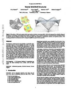
ing. Consequently the arches need to be stiff and can become quite massive structures. In contrast, the design concept for the Oleada main entrance structure at the Seville EXPO (Fig. 1) was intended to employ arches with a slender pin-jointed compression boom surrounded by a prestressed cable bracing system to provide adequate bending stiffness [2]. To sustain asymmetric loading due to cross winds however, the required torsional bracing became quite stiff and complex in the sense that separate rod members with close construction

Fig. 1.

Oleada main entrance structure at Seville EXPO.

0141-0296/01/$ - see front matter © 2000 Elsevier Science Ltd and Civil-Comp Ltd. All rights reserved. PII: S 0 1 4 1 - 0 2 9 6 ( 0 0 ) 0 0 0 1 9 - 5

30

S.M.L. Adriaenssens, M.R. Barnes / Engineering Structures 23 (2001) 29–36

Fig. 2. Perspective of Tensegrity Arch supporting large-span membrane.

tolerances would be required; entailing expensive joints and construction methods. The system was therefore abandoned in preference to the use of welded tubular arches. The main span of 80 m required tubes of 810 mm diameter; still slender, but far less so than the impression which would have been given by the cable braced system which required central compression booms of only 280 mm diameter. The ideas for the above system have since been revisited, and in particular the construction problems of potential lack-of-fit in members have been alleviated by a torsion free cable braced arch [3]. The system is illustrated in Figs. 2 and 3. Apart from simplifying construction, in the sense that only the longitudinal cable chords or potentially only one chord needs to be prestressed, the structural system is also more able to deform to accommodate loadings and avoid stress concentrations in the membrane — because of the torsional freedom the membrane stresses either side of the tensegrity arch equilibrate each other. Fig. 4 shows an extreme cross wind case demonstrating the stability of the system. Although the idea of pin-jointed boom members (with surrounding tensegrity yokes and cable bracing) may be attractive, and feasible for long spans, the cost of the

Fig. 3. Detail of Tensegrity Arch.

Fig. 4. Stability of Tensegrity Arch under extreme cross wind case.

pinned or sphere joints would still be high. For medium span systems it should be preferable to use a continuous tubular compression boom (rather than one which is cut into discrete lengths and then joined again). This idea of a less interrupted flow of direct (axial) forces is also crucial to the concept of grid shells with simple jointing of continuous members [4]; these are considered in a later section. However, to borrow another idea from grid shell systems, which are erected into a doubly curved form with lathes bent from an initially straight state, the central tubular boom in a medium span tensegrity arch might also be bent from straight. For larger spans a centre core bundle (for example of three tubes) might be used; the principal aim being to reduce the bending stiffness and stresses without reduction of the axial stiffness and strength. The bending stiffness is subsequently provided by prestressing out cable bracing around the central boom or core. The numerical form-finding of these systems requires a procedure which allows for the lengths or tensions of component links to be controlled either elastically or held at specified values. In addition, slip links are required in which forces in consecutive elements are equal; for example the tensions in one or more continuous cable chord members which during form-finding (and erection) may slide through the apex nodes of the triangular yokes; or compressions in adjacent links of the central tube or tube bundle may need to be equalised because the diagonal cables are attached to sliding collars. The latter would be required for systems which may be deployed and prestressed by drawing out a cable, yoke and collar system along the central boom. All of these features are readily incorporated in most tensile structures CAD systems, the simplest of which is probably a Dynamic Relaxation (DR) scheme which is summarised below, and described in detail in ref. [5]. A further aspect required, or at least desirable, in the numerical analysis is the treatment of the spline beams as a finite difference continuum, and this is developed in Section 3 of this paper.

S.M.L. Adriaenssens, M.R. Barnes / Engineering Structures 23 (2001) 29–36

with any applied load components, to give the updated residuals:

2. Dynamic relaxation numerical scheme The basis of the method is to trace step-by-step for small time increments, ⌬t, the motion of each node of a structure until, due to artificial damping, the structure comes to rest in static equilibrium. In form-finding the process may be started from an arbitrary specification of geometry, with the motion caused by imposing a stress or force specification in some or all of the structure components. The form-finding is usually carried out for a weightless state since, after obtaining an equilibrium state, this allows a subsequent factoring of the prestress forces in all components without affecting the geometry. For load analyses, which must start from the prestress equilibrium state, the motion is caused by suddenly applying the loading. The description of DR summarised briefly below for skeletal structures with strut and cable links assumes “kinetic” damping of the structural system to obtain a static equilibrium state [5]. In this procedure the undamped motion of the structure is traced and when a local peak in the total kinetic energy of the system is detected, all velocity components are set to zero. The process is then restarted from the current geometry and repeated through further (generally decreasing) peaks until the energy of all modes of vibration have been dissipated and static equilibrium is achieved. Newton’s second law governing the motion of any node i in direction x at time t is: Rtix⫽Mi.Vtix

⫽Pt⫹⌬t ⫹ Rt⫹⌬t ix ix

冘冉 冊 T L

t⫹⌬t

.(xj ⫺xi)t⫹⌬t

(4)

m

all links m connecting to i where Tm is the tension in link m connecting node i to an adjacent node j, and Lm is the current length of link m. The procedure is thus time stepped using Eqs. (2)–(4) until a kinetic energy peak is detected. Velocity components are then reset to zero (with a small adjustment made to the geometry to correct to the true kinetic energy time peak), and the process is repeated until adequate convergence. In skeletal structures the link tensions for use in Eq. (4) are given by: s s t+⌬t s T t+⌬t m ⫽T m⫹K m(L m ⫺Lm)

(5)

Where T sm,K sm,Lsm are respectively the “initial” or specified tension, elastic stiffness and length of a link m. In load analyses the initial state will be the prestress equilibrium geometry and tensions and K sm is the elastic stiffness; but in form-finding, any of the properties with superscript s can be used to control the form [6] — for example, tensions can be held constant by setting K to zero. (For continuous compression members with sliding collar nodes, compression throughout are based on elastic stiffness and overall contraction.)

(1)

where Rix is the residual force and Mi is the (fictitious) lumped mass at node i, which is set to optimise convergence and ensure stability of the numerical process [5]. Expressing the acceleration term in Eq. (1) in finite difference form and rearranging gives the recurrence equation for updating velocity components: Vt+⌬t/2 ⫽Vt−⌬t/2 ⫹ ix ix

31

⌬t t .R Mi ix

(2)

Whence the updated geometry projected to time (t+⌬t) is: xt+⌬t ⫽xti⫹⌬t.Vt+⌬t/2 i ix

(3)

Similar Eqs. (2) and (3) apply for all unconstrained nodes of the structure in each co-ordinate direction, and the equations are nodally decoupled in the sense that updated velocity components are dependent only on previous velocity and residual force components at a node. They are not directly influenced by the current (t+⌬t/2) updates at other nodes. Having obtained the complete updated geometry the new link forces can be determined and resolved, together

3. Spline beam elements The spline beam element described below is useful for modelling spline beams or grid shells employing continuous tubular members, and also for membranes in which flexible battens are employed to give shape control (usually for small span systems). It has significant advantages in a DR scheme since it requires only three translational degrees of freedom per node. Rotational degrees of freedom are not required, and it is often the coupling of these with axial stiffnesses and translational degrees of freedom, which can cause conditioning problems in explicit numerical methods such as DR. Furthermore, the treatment of sliding collars along continuous tubes is considerably simplified. The scheme adopted is, in effect, a finite difference modelling of a continuous spline beam traverse, and a similar scheme has been used for two-dimensional dynamic problems by Pian et al. [7]. Fig. 5a represents consecutive nodes along an initially straight tubular beam traverse, and Fig. 5b two adjacent deformed segments, a and b, viewed normal to the plane of nodes ijk which are assumed to lie on a circular arc of radius R. The spacings of nodes along the traverse must be sufficiently close to model this, but the segment lengths need not be equal.

32

S.M.L. Adriaenssens, M.R. Barnes / Engineering Structures 23 (2001) 29–36

vided the spline is initially straight and with EI constant about any axis: Considering an initially straight spline bent into a closed ring of radius R, and subject to equal and opposite loads P applied at the quarter points normal to the plane of the ring (Fig. 6): If the bending moment about a radial axis at A is M and the torsion at this location is T, then moment equilibrium about axes parallel to x and y through A gives: PR (1⫺ sin q)⫽M cosq⫹T sinq 2 Fig. 5. (a) Consecutive nodes along an initially straight tubular beam traverse; (b) Two adjacent deformed segments, a and b, viewed normal to the plane of nodes ijk.

and

(7)

PR (1⫺ cosq)⫽T cosq⫺M sinq 2

thus: From the geometry of Fig. 5b, the radius of curvature through i j k and the consequent Moment M are: R⫽

PR PR (sinq⫹cosq⫺1); M⫽ (cosq⫺ sinq) 2 2

(8)

dT and M⫽ dq

lc EI and M⫽ 2sina R

(Note that EI is assumed constant along the traverse) The free body shears of elements a and b are therefore: 2EI.sina 2EI.sina Sa⫽ ; Sb⫽ la.lc lb.lc

T⫽

(6)

These must be taken as acting normal to the chords and in the local plane of i j k. The calculations and transformations required in a DR scheme are thus very simple, with sets of three consecutive nodes being considered sequentially along the entire traverse; each set lying in different planes when modelling a spatial curve. If the traverse is pin-ended, as would normally be the case for traverses in grid shells, no special numerical treatment for end conditions is required. If the traverse is a closed loop then overlapping end segments are required. (A similar finite difference type of modelling would be required for fixed-ended traverses using extended end segments). If the stiffnesses used when setting nodal masses in the DR process [5] are unfactored, the minimum length of any traverse segment should not be less than the radius of gyration of the cross-section. In practice this limit is not likely to be approached; but if so, appropriate factoring of the bending stiffness must be applied when setting mass components in order to allow for coupling of the axial displacements with bending stiffnesses. Although the above analysis would clearly apply to a spline beam traverse bent into a single plane, with accuracy dependent only on the number of segments, it might be questioned whether it is applicable to a spatially twisted spline since apparently no torsional stiffness enters into the analysis; yet in fact this is the case pro-

but the prestressing moment (about an axis normal to the plane of the ring) is EI/R, and the component of this along the axis of T is: EI dw T⫽ . R Rdq

(9)

where w is the normal displacement. Differentiating this gives the full elastic stiffness moment: M⫽EI

d 2w R2dq2

(10)

Fig. 6. Closed Ring with equal and opposite loads P at the quarter points normal to the plane of the ring.

S.M.L. Adriaenssens, M.R. Barnes / Engineering Structures 23 (2001) 29–36

33

Thus the whole torsion T is due to the prestressing effect (of bending the initially straight spline tube into a closed ring), and there is no component due to twisting and the elastic torsion constant GJ. A more general proof for splines with uniform second moment of area bent into any spatial curve has been developed by Williams and is given in ref. [8]. Substituting T or M from Eq. (8) into Eq. (9) or Eq. (10), and integrating gives: PR3 w⫽ (⫺ cosq⫹sinq⫺q)⫹constant 2EI

(11)

If ⌬ is the displacement of the downward loads relative to the upwards loads then:

冉 冊

PR3 ⌸ ⌬⫽ 1⫺ EI 4

(12a) Fig. 7.

For the same ring, but unstrained in its initial circular state, the displacements(s) corresponding to the same out-of-plane loading can be shown to be:

冉 冊

PR3 ⌸ PR3 ⌬⫽ ⫺1 ⫹ (⌸⫺3) 2EI 2 2GJ

(12b)

It is interesting to note that the out-of-plane stiffness given by Eq. (12a) which is due principally to geometric stiffening by initial straining, is greater than that given by Eq. (12b) (in contrast, the in-plane-stiffness is identical for both, provided EI is the same).

4. Test cases 4.1. Out-of-plane loading of a closed ring The prestressed ring provides a useful test for examining convergence and the effect of unequal segment lengths. In the following, the ring is divided into four quadrants: 1–2, 2–3, 3–4, 4–1, with respectively: n, 2n, 4n, and 8n segments; Fig. 7 shows a subdivision density of n=2. The test ring has a diameter of 10 m, EI=100 kNm2, EA=100 MN, and loads of 1 kN applied in the z (normal) direction at nodes 1 and 3, with nodes 2 and 4 restrained in the z direction only. Table 1 gives values of normal displacement ⌬ at nodes 1 and 3 with increasing subdivision density n. For comparison, corresponding values ⌬e obtained using equivalent numbers of equal segments are also shown (n=8 corresponds to 120 segments). The fully converged solution of ⌬=0.2680 m is slightly stiffer than the figure of 0.2683 m given by Eq. (12a) due to the axial tension stiffening effect.

Ring with segments distributed non-uniformly.

4.2. Strut buckling into the elastica Buckling of a pin-ended strut into the elastica also provides a useful comparison for testing convergence of the numerical process. An appropriate analytical function and tabulated results defining the shape of the elastica (Fig. 8) are given by Timoshenko [9:79]. The numerical test example is a tubular strut of length L=10 m and the same section properties as used for the previous test case (Section 4.1). The strut, supported on end rollers and restrained to lie in the xy plane, is subject to increasing pairs of end axial loads, all above the Euler load. The four states of loading used for comparing the analytical results with numerical values obtained using increasing number of segments are shown in Fig. 9, and the results are tabulated in Table 2. The table gives x y values for and at the central node and shows good L L correlation and convergence. Note that state 4 is a particularly sensitive test: the end loads must be applied symmetrically and the model must remain symmetric at all stages, otherwise when it has passed through from state 3 to state 4 it is possible for the elastica to unwrap. For example when the load is applied at one end with the other end pinned, some lack of symmetry is induced during the numerical process. The system inverts to the stage shown in Fig. 10a but then unwraps around the pinned end to stage 10b and finally converges to a straight member in tension.

5. Applications The application of the foregoing spline analysis to tensegrity arches with continuous spline booms has been

34

S.M.L. Adriaenssens, M.R. Barnes / Engineering Structures 23 (2001) 29–36

Table 1 Normal displacements ⌬ for non-uniformly distributed segments and ⌬e for uniformly distributed segments with increasing subdivision density n

2

4

8

16

24

⌬ (m) ⌬e (m)

0.3009

0.2762 0.2698

0.2700 0.2684

0.2684 0.2680

0.2681 0.2680

Fig. 8.

Diagram showing,

x y and and P. L L

Fig. 10. (a) Elastica with load applied at one end, other end pinned during converging process; (b) Elastica unwraps around pinned end.

Fig. 9. Elastica in four buckled states. Table 2 Analytical and numerical values of displacement for central node of beam under four buckled states Buckled states Load

1 10.48 kN

2 12.67 kN

Central node

x/L

y/L

x/L

y/L

Analytical Numerical 8 segments 16 segments 32 segments 64 segments

0.4405

0.2110

0.2800

0.3595

0.4176 0.4363 0.4402 0.4413

0.2466 0.2184 0.2116 0.2099

0.2388 0.2752 0.2829 0.2848

0.3830 0.3630 0.3583 0.3572

referred to in Section 1, and indeed the three degree of freedom numerical procedure was developed in order to cater in a simple way with sliding collars along a bent spline (specifically, during deployment). Using a more normal six degree of freedom procedure (with both rotational and translational degrees of freedom at each node) would be complex when the lengths of member segments are effectively changing due to the sliding collars. Other useful applications of the numerical procedure are discussed in the following sections.

3 18.46 kN x/L

4 39.48 kN y/L

x/L

y/L

0.0615

0.4015

⫺0.1700

0.3125

⫺0.0194 0.0495 0.0614 0.0614

0.4080 0.4032 0.4022 0.4019

⫺0.2030 ⫺0.1916 ⫺0.1738 ⫺0.1699

0.3175 0.3077 0.3120 0.3130

5.1. Slender hoop rib supported membranes For prestressed membrane structures supported by circular arches, or slender hoop ribs, of radius R0 which are initially unstrained at this radius, the three degree of freedom spline analysis can be used provided “initial state” shears S1 and S2 are applied to the two end segments throughout the analysis, as shown in Fig. 11. In order to allow for rigid body rotations of the circular arc during analyses (when calculating nodal residuals) these

S.M.L. Adriaenssens, M.R. Barnes / Engineering Structures 23 (2001) 29–36

Fig. 11. Shear forces S1 and S2 are applied to the two end segments throughout the analysis for circular arches initially unstrained.

shears must always be applied in the plane containing the two end vectors ␫1 and ␫2. Note that if these shears were applied to the end segments of an originally straight spline, all nodes along the spline would lie exactly on an arc of radius R0; the shears are required in the analysis to give the initial arc state, and although it is clearly highly strained in this state, all of the interior shears cancel — so the effect is the same as an unstrained arc. When calculating in-plane moments at the end of an analysis the effect of R0 must obviously be accounted for using M=EI(1/R⫺1/R0), where R is the local radius of the deformed arc. Out-of-plane moments are determined using displacements normal to the average plane of the deformed arc. The analysis for unstrained arcs (rather than arcs bent from straight) is clearly approximate since the value of EI would correspond to the stiffness in only one direction (e.g. the radial direction for in plane bending), but it is useful for structures such as battened or hoop supported membranes. For both of these systems bending or snap through bucking behaviour is significant in only one direction — radially for hoop supported systems and normal to the (average) membrane plane for battened systems.

35

grid enable the dominant membrane stiffness to be gained after light prestressing. The concepts of the tensegrity arch referred to in Section 1 can be extended to two-way spanning double layer grids as shown in Fig. 12a and b. The two sets of tubular members can be either straight or bent from straight by prestressing the cable bracing system to form a curved structure. The cables are braced apart by flying struts and the tubular members are continuous with sliding collars to which the diagonal bracing is attached. The latter could enable deployment of the system from an initial bundled state with the tubes extended by slotting on additional sections as the cable bracing system is drawn out. Physical and numerical studies of these systems are being undertaken at the University of Bath, Department of Architecture and Civil Engineering [11].

6. Concluding remarks The bending routine explained in this paper is based upon a translational three degree of freedom approach

5.2. Grid shells In numerically modelling the form and behaviour of grid shell structures, one approach is to derive an initial form by means of a hanging funicular net [10] and subsequently to analyse the structure for various load states with a model employing six degrees of freedom at each node [4]. These analyses should clearly include the initial curvature from straight as an initial strain state, and indeed the correct initial self weight geometry can only be accurately obtained when this is accounted for. Grid shells are a particular class of structure in which a two-way grid of continuous members is deployed from straight, and the foregoing analysis provides an elegant technique for their form-finding and analysis. Conventionally they are single layer systems, although the continuity of members through nodes necessitates a finite separation of the two sets of grid members, with a connector between. Diagonal cables lying in the mean plane of the

Fig. 12. (a) Two-way spanning double layer tensegrity grid computer model; (b) Two-way spanning double layer tensegrity grid physical model.

36

S.M.L. Adriaenssens, M.R. Barnes / Engineering Structures 23 (2001) 29–36

developed for spatially curved continuous tubular splines bent from straight. The results for the test cases of a ring bent normal to its initial plane and a strut buckling into the elastica have demonstrated the stability and convergence of the process within a DR scheme. The method is particularly useful when applied to systems such as grid shells and cable braced splines with sliding collars. References [1] Ishii K. Membrane designs and structures in the world. Tokyo: Shinkenchiku-sha Co. Ltd, 1999. [2] Barnes MR, Renner W, Kiefer M. Case studies in the design of wide-span EXPO structures. In: Conceptual design of structures. Stuttgart: IASS, October 1996:814–821. [3] Adriaenssens SML, Barnes M, Mollaert M. Deployable torsion free tensegrity spines. Conf. Engineering and New Architecture. Denmark: Aarhus, May 1998:93–101.

[4] Happold E, Liddell WI. Timber lattice roof for the Mannheim Bundesgartenshau. The Struct Engr 1975;53:99–135. [5] Barnes MR. Form and stress engineering of tension structures. Struct Engng Rev 1994;6(3/4):175–202. [6] Barnes MR. Form-finding and analysis of prestressed nets and membranes. Comp Struct 1988;30(3):685–95. [7] Pian THH, Balmer HA, Bucciarelli LL. Dynamic buckling of a circular ring constrained in a rigid circular surface. In: Herrmann G, editor. Int. Conf. on Dynamic Stability of Structures. Illinois, 1965. [8] Adriaenssens SML, Barnes MR, Williams CJK. A new analytic and numerical basis for the form-finding and analysis of spline and gridshell structures. In: Kumar B, Topping BHV, editors. Computing developments in civil and structural engineering. Edinburgh: Civil-Comp Press, 1999:83–90. [9] Timoshenko SP. Theory of elastic stability. New York: McGrawHill Book Company, 1961. [10] Frei Otto, Grid Shells IL10, Stuttgart, 1974:180–181. [11] Adriaenssens SML, Keverne M, Stessels S. Research reports on studies in the modelling of tensegrity grid shells. The University of Bath, 1998 and 1999.