Tensor-based methods for system identification

9th International conference on Sciences and Techniques of Automatic control & computer engineering

Tensor-based methods for system identification Gérard Favier1 and Alain Y. Kibangou2 1

Laboratoire I3S, University of Nice Sophia Antipolis, CNRS, Les Algorithmes- Bât. Euclide B, 2000 Route des lucioles, B.P. 121 - 06903 Sophia Antipolis Cedex, France [email protected] 2 LAAS-CNRS, University of Toulouse, 7 avenue Colonel Roche, 31077 Toulouse, France [email protected]

Abstract. This paper first aims at introducing the main notions relative to tensors, also called multi-way arrays, with a particular emphasis on tensor models, uniqueness properties, tensor matricization (also known as unfolding) and the alternating least squares (ALS) algorithm that is the most used method to estimate the matrix components of a tensor. The interest for tensors in signal processing will be illustrated by means of some examples (tensors of statistics, Volterra kernels, tensors of signals), and we will show how a tensor approach allows to solve the parameter estimation problem for both linear and nonlinear models, by means of deterministic or stochastic methods. Key words: Tensor models; System identification.

1

Brief historic review and motivations

The word tensor was introduced in 1846 by William Rowan Hamilton, irish mathematician famous for his discovery of quaternions and very well known in the automatic control community for his theorem (Cayley-Hamilton’s theorem) stating that any square matrix cancels its characteristic polynomial. The tensor notion and the tensor analysis began to play an important role in Physics with the introduction of the theory of relativity by Albert Einstein, around 1915, then in mechanics for representing the constraint and deformation state of a volume subject to forces by means of a stress tensor and a deformation tensor respectively. Tensor decompositions were introduced by Hitchcock in 1927 [1], then developed and applied in psychometrics by Tucker [2] in 1966, and Carroll and Chang [3] and Harshman [4] in 1970, who introduced the most common tensor models, respectively called Tucker, CANDECOMP and PARAFAC models. Such tensor models became very popular tools in chemometrics in the nineties [5]. Tensors, also called multi-way arrays, are very useful for modeling and interpreting multidimensional data. Applications of tensor tools can now be found in many scientific areas, including image processing, computer vision, numerical analysis, data mining, neuroscience and many others. Tensors first appeared in signal processing (SP) applications in the context of the blind source separation problem solved in using cumulant tensors [6, 7]. Indeed, moments STA'2008-SP-001, pages 1-36 Academic Publication Center of Tunis, Tunisia

2

and cumulants of random variables or stochastic processes can be viewed as tensors [8], as will be illustrated later on by means of some examples. First SP applications of the PARAFAC model were made by Sidiropoulos and his co-workers in the context of sensor array processing [9] and wireless communication systems [10], in 2000. The motivation for using tensor tools in the SP community was first connected to the development of SP methods based on the use of high-order statistics (HOS). Another motivation follows from the multidimensional nature of signals, as it is the case, for instance, with the emitted and received signals in wireless communication systems [11]. Another illustration is provided by the kernels of a Volterra model. The tensor algebra, also called multilinear algebra, constitutes a generalization of linear algebra. Whereas this last one is based on the concepts of vectors and vector spaces, the multilinear algebra relies upon the notions of tensors and tensor spaces. As matrices arise for representing linear applications, the tensors are associated with the representation of multilinear applications. Nowadays, there exist several mathematical approaches for defining a tensor. In a simplified way, a tensor can be viewed as a mathematical object described by means of a finite number of indices, this number being called the tensor order, and satisfying the multilinearity property. So, a tensor H ∈ K I1 ×I2 ×···×In , of order n, with elements in the field K = ℜ or C , depending on whether the tensor elements are real-valued or complex-valued, and dimensions (I1 , I2 , · · · , In ), will have for entries hi1 i2 ···in with i j = 1, 2, · · · , I j , j = 1, 2, · · · , n. Each index i j is associated with a coordinate axis, also n

called a mode or a way. The tensor H is characterized by ∏ I j elements, also called j=1

coefficients or scalar components. Particular cases – A scalar h is a tensor of order zero (without index). – A vector h ∈ K I is a first-order tensor, with coefficients hi , i = 1, · · · , I, and a single index. – A matrix H ∈ K I×J is a second-order tensor, with coefficients hi j and two indices. – A third-order tensor, also called a three-way array, H ∈ K I×J×K , of dimensions I × J × K, with entries hi jk , can be viewed as a hyper rectangle, the indices i, j, and k being associated with the horizontal, lateral, and frontal coordinate axes (modes) respectively (see Fig. 1). Fig. 1 represents a third-order tensor with its decompositions in matrix slices (two-dimensional sections of the tensor, also called slabs) obtained by slicing the tensor along each mode, i.e. by fixing an index and varying the two other ones. The horizontal, lateral, and frontal slices of a third-order tensor H are denoted by Hi.. , H. j. , and H..k respectively. In the sequel, vectors and matrices are represented by boldface lowercase (x) and boldface capital (X) letters, respectively, whereas tensors are denoted by capital blackboard letters (X).

3

H

Mode 1 i=1,...,I

Mode 3 k=1,...,K

Mode 2 j=1,...,J

i=1,...,I

H.1. H.j.

H.J.

HI..

...

Mode 1 fixed

j=1,...,J

... ... H..1

...

... ...

...

Hi..

...

H1..

... ...

Matricization

Mode 2 fixed

H..K H..k

...

... k=1,...,K

Mode 3 fixed Fig. 1. Geometrical representation and slice decompositions of a third-order tensor.

4

Symmetric and diagonal tensors A third-order tensor X is said to be square if every mode has the same dimension I, i.e. X ∈ K I×I×I . A square third-order tensor X ∈ K I×I×I is said to be symmetric if its elements do not change under any permutation of its indices, i.e.: xi jk = xik j = x jik = x jki = xki j = xk ji , ∀ i, j, k = 1, ..., I. A third-order tensor X can be partially symmetric in two modes. For instance, X is symmetric in the modes i and j if its frontal slices X..k are symmetric matrices. A third-order tensor X is diagonal if xi jk 6= 0 only if i = j = k. The diagonal tensor with ones on its superdiagonal is called the identity tensor. The above definitions can be easily extended to tensors of any order n > 3.

2 Examples of tensors in SP 2.1

Tensors of statistics

Third-order cumulants of three real vector random variables Let x, y, and z be three real-valued vector random variables, of respective dimensions M1 , M2 , and M3 . The cumulant Cx,y,z = cum(x, y, z) is a third-order tensor, with elements [Cx,y,z ]m1 ,m2 ,m3 = cum(xm1 , ym2 , zm3 ). The modes 1, 2, and 3 correspond to the components of each vector x, y, and z respectively. Fourth-order cumulants of a real scalar stochastic process Let x(k) be a discrete-time, stationary, real-valued, scalar stochastic process. Its fourthorder cumulants define a third-order tensor, with entries [C4x ]τ1 ,τ2 ,τ3 = cum(x(k), x(k − τ1 ), x(k − τ2 ), x(k − τ3 )). The modes 1, 2, and 3 are associated with the time lags τ1 , τ2 , and τ3 . Spatio-temporal covariances of a real-valued vector stochastic process Let x(t) ∈ ℜM be the vector of signals received on an M sensor array, at¤the time instant £ t. The spatio-temporal covariance matrices Cxx (k) = E x(t + k)xT (t) , k = 1, · · · , K, define a third-order M × M × K tensor, with entries [Cxx ]i, j,k = E [xi (t + k)x j (t)]. The two first modes i and j are spatial (sensor numbers) whereas the third mode k is temporal (covariance time lag).

5

Third-order space cumulants of a real-valued vector stochastic process Let x(t) ∈ ℜM be the vector of signals received on an M sensor array, at the time instant t. The third-order space cumulants cum(x, x, x) define a third-order M × M × M tensor Cxxx , with elements [Cxxx ]i, j,k = cum (xi (t), x j (t), xk (t)). The three modes i, j, and k are spatial, the signals being considered at the same time instant t. 2.2

Kernels of Volterra models

SISO Volterra models A P-th order Volterra model for a single-input single-output (SISO) system, is given by: P

y(n) = h0 +

Mp

∑ ∑

Mp

p=1 m1 =1

···

∑

p

m p =1

h p (m1 , · · · , m p ) ∏ u(n − m j ) j=1

where u(n) and y(n) denote respectively the input and output signals, P is the nonlinearity degree of the Volterra model, M p is the memory of the pth-order homogeneous term, and h p (m1 , · · · , m p ) is a coefficient of the pth order kernel. This kernel can be viewed as an pth order M p × Mp × · · · × Mp tensor. MIMO Volterra models In the case of a multi-input multi-output (MIMO) Volterra model, with u(n) ∈ ℜnI and y(n) ∈ ℜnO , where nI and nO denote respectively the number of inputs and outputs, the input-output relationship, for s = 1, ...no , is given by: ys (n) = hs0 +

P

nI

nI

p=1 j1 =1

Mp

Mp

∑ ∑ ··· ∑ ∑

j p =1 m1 =1

···

∑

m p =1

p

hsj1 ,··· , j p (m1 , · · · , m p ) ∏ u jk (n − mk ) k=1

where hsj1 ,··· , j p (m1 , · · · , m p ) is the kernel of the sth output, acting on the product of p delayed input signals (with time delays m1 , · · · , m p ), these signals being possibly associated with different inputs ( j1 , · · · , j p ). This Volterra kernel is now of order 2p and dimensions Mp × · · · × Mp × nI × · · · × nI with p temporal modes corresponding to the delays m1 , · · · , m p and p space modes associated with inputs j1 , · · · , j p . 2.3

Tensors of signals

Signals received by a communication system oversampled at the receiver The signals received on an M antennas array, with an oversampling rate equal to P, and over a time duration of N symbol periods, constitute a tensor X ∈ C M×N×P , with entries xm,n,p , m = 1, · · · , M, n = 1, · · · , N, p = 1, · · · , P, the three modes being associated with an antenna number (m), a symbol period (n), and an oversampling period (p).

6

Signals received by a CDMA (Code Division Multiple Access) system At the transmitter, each symbol to be transmitted is spread by means of a spreading code of length J, with a period Tc = T /J, where T is the symbol period. So, each symbol is converted into J chips. A block of N signals received by M antennas can then be viewed as a third-order tensor X ∈ C M×N×J , with entries xm,n, j , m = 1, · · · , M, n = 1, · · · , N, j = 1, · · · , J. Signals received by an OFDM (Orthogonal Frequency Division Multiplexing) system In an OFDM system, the symbol sequence to be transmitted is organized into blocks of F symbols in the frequency domain. In this case, the received signals constitute a thirdorder tensor X ∈ C M×N×F , with entries xm,n, f , m = 1, · · · , M, n = 1, · · · , N, f = 1, · · · , F. We can conclude that these three received signals have two modes in common (m and n), and differ from one another in the third mode (p, j, or f ). An unified tensor model of PARAFAC type was put in evidence for these three communication systems [11].

p, j, or f m

n

X

Mode 1 m=1,..., M

Mode 2 n=1,..., N

Mode 3 p=1,..., P or j=1,..., J or f=1,..., F

Fig. 2. Tensors of signals received by the three communication systems.

For illustrating these tensors of received signals, let us consider the case of a CDMA system [10]. In presence of Q users and in absence of noise, the signal received by the m-th antenna (m = 1, · · · , M), at the n-th symbol period (n = 1, · · · , N), can be written as: Q

xm,n, j =

∑ amq snq c jq

q=1

(1)

7

where amq denotes the fading coefficient of the channel between the q-th user and the m-th receive antenna, snq is the symbol transmitted by the q-th user, at the n-th symbol period and using the j-th spreading code c jq . The set of signals received by the M receive antennas, during N symbol periods and using J spreading codes per user, constitutes a third-order tensor X ∈ C M×N×J . Equation (1) corresponds to a PARAFAC model ( See Section 4.1).

3 Some recalls on matrices and matrix decompositions In this section, we recall some definitions relative to matrices and some matrix decompositions. For a matrix A ∈ C I×J , we denote by Ai. and A. j its i-th row vector and j-th column vector respectively. 3.1

Column-rank and row-rank

For a matrix A ∈ ℜI×J , the number of linearly independent rows (columns) of A is called the row-rank (column-rank) of A. The row-rank and the column-rank of a matrix are equal. This number, denoted by r(A), is called the rank of A. We have: r(A) ≤ min(I, J) – A is said to be full rank if r(A) = min(I, J) and rank-deficient if r(A) < min(I, J). – A is said to be full column-rank if r(A) = J, i.e. if the J columns are independent. – Analogously, A is said to be full row-rank if r(A) = I, i.e. if the I rows are independent. For a square matrix A ∈ ℜI×I , if r(A) < I, then det(A) = 0 and A is called singular; if A is full-rank, then det(A) 6= 0 and A is called nonsingular. For A ∈ ℜI×J , we have:

r(AAT ) = r(AT A) = r(A)

For any full column-rank matrix C and full row-rank matrix B, with appropriate dimensions, we have : r(A) = r(AB) = r(CA) = r(CAB). A rank-one matrix A can be written as the outer product of two vectors: A = u ◦ v = uvT where the symbol ◦ denotes the vector outer product defined as follows: u ∈ ℜI , v ∈ ℜJ → u ◦ v ∈ ℜI×J ↔ (u ◦ v)i j = ui v j

8

3.2

The rank theorem

For any matrix A ∈ ℜI×J , we have: dimR(A) + dimN (A) = J where R(A) = {Ax/x ∈ ℜJ } is the column space, also called the range space, of A, and N (A) = {x/Ax = 0} is the nullspace of A, with dimR(A) = r(A). From this theorem, we can conclude that: – If A is full column-rank (dimR(A) = J), we have dimN (A) = 0 and consequently N (A) = {0}. – If A is rank-deficient (dimR(A) < J), we have dimN (A) > 0, which implies N (A) 6= {0}. 3.3

k-rank (or Kruskal-rank)

The notion of k-rank was introduced by Kruskal [12] for studying the uniqueness of the PARAFAC decomposition of a given tensor. Consider a matrix A ∈ ℜI×J of rank r(A). The k-rank of A is the largest integer k such that any set of k columns of A is independent. It is denoted by kA . The k-rank is more constraining than the column-rank in the sense that kA = k means that any set of k columns of A is independent, whereas r(A) = k implies that there exists at least one set of k independent columns and any set of k + 1 columns is dependent. So, we have: kA ≤ r(A). – If A ∈ ℜI×J is full column-rank, then kA = J. – If A ∈ ℜI×J has no all-zero column, but contains at least two proportional columns, then kA = 1. – If A ∈ ℜI×J has an all-zero column, then kA = 0. Examples  111 A1 = 1 1 0 ⇒ r(A1 ) = 2, kA1 = 1 110   101 A2 = 0 1 1 ⇒ r(A2 ) = kA2 = 2 000   100 A3 = 0 1 0 ⇒ r(A3 ) = 2, kA3 = 0 000 

9

3.4

The vectorization operator vec(.)

The vec-operator put the matrix A ∈ K I×J in the form of a column vector of dimension IJ, denoted by vec(A), by stacking all the column vectors of A:   A.1 ¡ ¢  ..  I×J A = A.1 · · · A.J ∈ K ⇒ vec(A) =  .  ∈ K IJ A.J

The matrix A is said to be vectorized, and we have:

v = vec(A) ⇔ v(i−1)J+ j = ai j . 3.5

Kronecker and Khatri-Rao products

These matrix products are used for matricizing tensors. The Kronecker product of two matrices A ∈ K I×J and B ∈ K is the partitioned matrix C ∈ K IK×JL defined as:   a11 B a12 B · · · a1J B a21 B a22 B · · · a2J B   C = A⊗B =  . ..  .. . .  .. . .  .

K×L ,

denoted by A ⊗ B,

aI1 B aI2 B · · · aIJ B

The Kronecker product of two vectors u ∈ ℜI and v ∈ ℜJ is the vector w ∈ ℜIJ such that: w(i−1)J+ j = ui v j The Khatri-Rao product of two matrices A ∈ K I×J and B ∈ K K×J having the same number of columns, is the IK × J matrix denoted by A ⊙ B and defined as: ¡ ¢ A ⊙ B = A.1 ⊗ B.1 A.2 ⊗ B.2 · · · A.J ⊗ B.J (2)

This product is also called the column-wise Kronecker product. It can be written in the form of I row-blocks:  A BD1 BDA   2 A⊙B =  .  (3)  ..  BDA I

matrix, ¢with the elements of the i-th row of A on its main diagwhere DA i is a diagonal ¡ a a · · · aiJ . onal: DA = diag i1 i2 i

We have the following properties: for v ∈ K J , A ∈ K vec(ABC) = (CT ⊗ A)vec(B) T

I×J ,

B∈K

J×K ,

C∈K

vec(Adiag(v)B) = (B ⊙ A)v ¡ ¢ ¡ ¢ (Adiag (v)) ⊙ BT = A ⊙ BT diag (v) = A ⊙ BT diag (v)

K×L ,

(4) (5) (6)

10

where the operator diag(.) forms a diagonal matrix from its vector argument. For A ∈ K

I×R

and B ∈ K

J×R ,

we have:

r(A ⊙ B) ≤ r(A ⊗ B) = r(A)r(B) and if neither A nor B contains a zero column [13]: kA⊙B ≥ min(kA + kB − 1, R) As a consequence, we have [9]: A ⊙ B is full column-rank if kA + kB ≥ R + 1. We have to note that: – This condition is satisfied, in particular, if one matrix is full column-rank R and the other one contains no zero column. – This condition implies I + J ≥ R + 1 and therefore IJ ≥ R, i. e. A ⊙ B is tall. 3.6

Moore-Penrose matrix pseudo-inverse

The Moore-Penrose pseudo-inverse of a matrix A ∈ K A† , that satisfies the four following conditions: AA† A = A,

A† AA† = A† ,

I×J

(AA† )T = AA† ,

is a J × I matrix, denoted by (A† A)T = A† A.

The Moore-Penrose pseudo-inverse always exists and is unique. See its expression in terms of the SVD in the next section. If A ∈ C I×J is full column rank, its Moore-Penrose pseudo-inverse is given by: A† = (AH A)−1 AH . The calculation of A† needs to inverse a J × J matrix. If A is a nonsingular matrix, then A† = A−1 . 3.7

Principal component analysis (PCA)

Consider a matrix A ∈ ℜI×J . Ifªr(A) = R, then there exists a set of R pairs of vectors © I ur ∈ ℜ , vr ∈ ℜJ ; r = 1, · · · , R such that: R

A=

∑ ur vTr =

r=1

R

∑ ur ◦ vr

(7)

r=1

The scalar writing of this matrix decomposition is the following: R

ai j =

∑ uir v jr ,

r=1

i = 1, · · · , I, j = 1, · · · , J.

(8)

11

This writing corresponds to a bilinear decomposition of A by means of R components, each term ur vTr , called a dyad, being a rank-one matrix. That means that any matrix of rank R can be written as a sum of R rank-one matrices. The decomposition (7) is called a PCA model of A. It can also be written as: ¡ ¢¡ ¢T A = UVT = u1 · · · uR v1 · · · vR , with U ∈ ℜI×R , V ∈ ℜJ×R .

(9)

The set of vectors {ur , vr ; r = 1, · · · , R} is not unique. Indeed, for any nonsingular ma¯ = UΛ and V ¯ = VΛ −T are such that: trix Λ , the matrices U ¡ ¢ ¯V ¯ T = UΛ VΛ −T T = UVT . U

The only uniqueness case (up to a scaling factor) occurs when A is of rank one. Uniqueness can be obtained in imposing structural constraints on the matrix factors U and V (orthogonality, Toeplitz, Vandermonde, constant modulus, finite alphabet).

3.8

Singular value decomposition (SVD) and PCA

Given matrix A ∈ ℜI×J with rank R, its reduced SVD is: A = UR SR VTR , ¡ ¢ ¡ ¢ where UR = u1 · · · uR ∈ ℜI×R and VR = v1 · · · vR ∈ ℜJ×R are column-orthonormal matrices and SR ∈ ℜR×R is diagonal: UTR UR = VTR VR = IR

;

¢ ¡ SR = diag σ1 · · · σR

where the σi > 0, i = 1, · · · , R, are the nonzero singular values of A, that are the positive square roots of the nonzero eigenvalues of AT A (and also of AAT ), the columns ui of UR are the eigenvectors of AAT , also called the left singular vectors of A, whereas the columns vi of VR are the eigenvectors of AT A, also called the right singular vectors of A. Equivalently, we have: R

A=

∑ σr ur vTr ,

(10)

r=1

which shows that the SVD decomposes A into R rank-1 matrices. Consequently, the rank of A is the smallest number R of rank-1 matrices whose the sum equals A. By defining U = UR SR and V = VR , we find again the PCA decomposition (9) with the column orthogonality constraint on the factors. The Moore-Penrose pseudo-inverse of A is given by: T A† = VR S−1 R UR .

12

3.9

LS solutions of a set of linear equations

The least squares (LS) solutions of the set of linear equations Ax = y, with x ∈ ℜJ , y ∈ ℜI , A ∈ ℜI×J , are such that kAx − yk22 is minimized with respect to x. The LS solutions, denoted by xˆ LS , are solutions of the normal equations: AT AˆxLS = AT y. It is important to mention that, even if the set of equations Ax = y is inconsistent, i.e. it admits no exact solutions, which corresponds to y ∈ / R(A), the set of normal equations AT Ax = AT y is always consistent, i.e. it always admits at least one solution [14]. Indeed, AT y ∈ R(AT ) = R(AT A) implies that the second member of the normal equations belongs to the column space of its coefficient matrix (AT A), which is the condition to satisfy for ensuring the consistency of a system of linear equations. The LS solution is unique if and only if A is full column-rank. In this case, we have: xˆ LS = (AT A)−1 AT y = A† y

(11)

When A is rank-deficient, there exists an infinite number of LS solutions and the general solution of the normal equations is given by: xˆ LS = A† y + (I − A† A)z

(12)

where z is any vector of ℜJ . The second term of this sum belongs to the nullspace of A, which means R(I − A† A) = N (A). Indeed, we have: A(I − A† A)z = (A − AA† A)z = 0 and consequently: ¡ ¡ ¢ ¢ AT AˆxLS = AT A A† y + I − A† A z = AT AA† y = AT AA† Ax = AT Ax = AT y

which shows that xˆ LS defined in (12) satisfies the normal equations.

We have to note that xˆ LS = A† y is the LS solution of minimal Euclidean norm. 3.10

Low-rank approximation of a matrix using its SVD[15]

Let us consider a matrix A ∈ ℜI×J of rank R, admitting UR SR VTR as reduced SVD, with the singular values σ1 ≥ σ2 ≥ · · · ≥ σR > σR+1 = · · · = σmin(I,J) = 0 and denote by kAk2F its Frobenius norm3 . Its best rank-K approximation (K ≤ R), in the sense min kA − Bk2F , is given by the sum of the K rank-one matrices of its SVD (10) B/r(B)=K

associated with the K largest singular values: K

AK =

∑ σk uk vTk

k=1 3

The Frobenius norm of

A ∈ ℜI×J

is defined as: kAk2F = ∑ a2i j = trace(AT A). i, j

13

and we have kA − AK k2F =

R

∑ σk2 .

k=K+1

This property is not valid for higher-order tensors.

4 Main tensor models It is important to notice that, in SP applications, tensor models are generally deduced from the underlying structure of the system under study and not from algebraic transforms applied to the data tensors. So, in the sequel, we will use the terms tensor model (also called multiway model or multilinear model) instead of tensor decomposition. We first present the most well-known and used tensor model, the so called PARAFAC (Parallel Factor) model. Then, we will briefly describe several other tensor models (Tucker, PARATUCK2, CONFAC). 4.1

The PARAFAC model

The following decomposition of the third-order tensor X ∈ ℜI×J×K : R

xi jk =

∑ air b jr ckr ,

r=1

i = 1, · · · , I, j = 1, · · · , J, k = 1, · · · , K,

(13)

is called the PARAFAC decomposition of X. Equation (13) is a generalization of equation (8) to the third-order. It is a trilinear decomposition with R components that can be also written as: R

X=

∑ A.r ◦ B.r ◦ C.r , with A ∈ ℜI×R , B ∈ ℜJ×R , C ∈ ℜK×R .

(14)

r=1

Each term of the sum, called a triad, is a third-order rank-one tensor, i.e. the outer product of three vectors, also called an indecomposable tensor. So, PARAFAC corresponds to a decomposition of the tensor into a sum of R rank-one tensors. This is illustrated in Fig.3 . The column vectors A.r , B.r , and C.r are of respective dimensions I, J, and K. They contain the coefficients air , b jr , and ckr of the three matrix factors (also called loadings or components) A, B, and C of the PARAFAC decomposition. The PARAFAC model can be easily extended to any order N > 3: R

xi1 i2 ...iN =

∑ ∏ ain r , in = 1, ..., In , n = 1, ...N, (n)

r=1 n

or equivalently R

X=

∑ A.r

r=1

(1)

(2)

(N)

◦ A.r ◦ · · · ◦ A.r , with A(n) ∈ C In ×R , n = 1, · · · , N.

(15)

14

K I

X

C.1 B.1

C.R B.R + ... +

= A.1

A.R

J Fig. 3. PARAFAC decomposition of a third-order tensor.

In certain applications, the matrix factors are used to interpret the underlying information contained in the data tensors. In other applications, these factors contain the information of interest on the system under study. So, in wireless communication applications, tensors of transmitted and received signals are decomposed into matrix factors that contain both the structure (design) parameters and the information of interest on the communication system. For instance, with future multiuser MIMO systems where a base station will simultaneously transmit data via multiple transmit antennas to several users equipped with multiple receive antennas, tensor modeling can be used for block space-time spreading, i.e. each data stream is spread across both space (antennas) and time (symbols) dimensions [16]. In this case, the design parameters corresponding to the tensor dimensions, are the number of transmit/receive antennas, the temporal spreading factor (number of spreading codes), the number of data streams transmitted per block, and the number of symbol periods, whereas the information of interest to be recovered concerns the channel, the transmitted symbols and eventually the spreading codes. In the case of tensor-based blind identification methods for FIR linear systems, like the ones described in sections 5.1 and 5.2 that are based on the use of fourth-order output cumulants, the cumulant tensor admits a PARAFAC model that is directly obtained from the transformation of the output signals into fourth-order cumulants. In the same way, with the tensor-based approach for Wiener-Hammerstein nonlinear system identification, presented in section 5.4, the tensor corresponding to the thirdorder Volterra kernel associated with the Wiener-Hammerstein system to be identified, admits a PARAFAC model that directly results from the underlying structure of the original nonlinear system. It is important to notice that the PARAFAC model captures the trilinear structure in the data, but this model is linear in its parameters, i.e. the coefficients of each matrix factor. This property is exploited in the ALS algorithm for estimating the PARAFAC parameters (see section 4.4).

15

In practice, a tensor of data is always represented as the sum of two terms : a structural term corresponding to the tensor model and a residual term containing both the measurement noise and the modeling error, which means that (13) is in general replaced by: R

xi jk =

∑ air b jr ckr + ei jk ,

r=1

i =, · · · , I, j = 1, · · · , J, k = 1, · · · , K,

where ei jk denotes the components of the residual tensor E. An analysis of these residuals allows to quantify the fit of the tensor model with the data. The sum of squares of these residuals ( kEk2F = ∑ e2i jk ) is often used as an objective function for estimating i, j,k

the PARAFAC parameters, and as a test for stoping the ALS algorithm. Tensor rank The rank of a third-order tensor X ∈ ℜI×J×K is the smallest number R of trilinear factors in its PARAFAC decomposition, i.e. the smallest number R such that (13) is exactly satisfied. Other definitions exist for the rank of a tensor: symmetric rank, maximum rank, typical rank, generic rank. Any symmetric tensor X ∈ C I×I×···×I of order N can be decomposed as a sum of R symmetric rank-1 tensors [17]: R

X=

∑ A.r ◦ A.r ◦ · · · ◦ A.r ,

(16)

r=1

with the matrix factor A ∈ C I×R . The symmetric rank (over C ) is defined as the minimum number R of symmetric rank-1 factors in the decomposition (16). The maximum rank is defined as the largest achievable rank for a given set of tensors. For instance, the set of all third-order tensors X ∈ ℜI×J×K has a maximum rank, denoted by Rmax (I, J, K), such that [18]: max(I, J, K) ≤ Rmax (I, J, K) ≤ min(IJ, IK, JK). Typical and generic ranks of tensors are more abstract concepts that are outside the scope of this paper ( See [19]). Remarks – Unlike matrices, the rank of a tensor can be larger than its largest dimension, i.e. R can be larger than max(I, J, K). – Kruskal [18] showed that the maximum possible rank of a third-order 2 × 2 × 2 tensor is equal to 3.

16

– The maximum possible rank of a third-order 3 × 3 × 3 tensor is equal to 5. – From a practical point of view, the rank of a tensor is difficult to determine. Uniqueness properties Uniqueness is a key property of the PARAFAC decomposition. Four kinds of uniqueness can be defined [20]: – Strict uniqueness: The matrix factors can be obtained without any ambiguity. – Quasi-strict uniqueness: The matrix factors can be obtained up to column scaling. – Essential uniqueness: The matrix factors can be obtained up to column permutation and scaling. – Partial uniqueness: One or two matrix factors are essentially unique, while the other(s) matrix factor(s) is (are) not. Consider the third-order tensor X ∈ ℜI×J×K . The PARAFAC decomposition of X is ¯ B, ¯ of the ¯ C) said to be essentially unique if two sets of matrix factors (A,B,C) and (A, PARAFAC decomposition are linked by the following relations: ¯ = AΠ ∆ 1 , A

¯ = CΠ ∆ 3 , B¯ = BΠ ∆ 2 , C ¡ i ¢ i , i = 1, 2, 3, are diagonal where Π is a permutation matrix, and ∆ i = diag d11 · · · dRR matrices such that: 1 2 3 ∆ 1∆ 2∆ 3 = IR , i.e. drr drr drr = 1, r = 1, · · · , R.

These permutation and scaling ambiguities are evident from the writings (13) or (14). The permutation matrix Π is associated with a reordering of the rank-one component tensors, whereas the diagonal matrices ∆ i , i = 1, 2, 3, correspond to a scaling of the 1 , d 2 , and d 3 respectively, so that columns A.r , B.r , and C.r by the diagonal elements drr rr rr the PARAFAC decomposition can be rewritten as: R

X=

∑ (drr1 A.r ) ◦ (drr2 B.r ) ◦ (drr3 C.r ).

r=1

The first uniqueness results are due to Harshman [4, 21]. The most general sufficient condition for essential uniqueness is due to Kruskal [12, 18] and depends on the concept of k-rank. Kruskal’s theorem A sufficient condition for essential uniqueness of the PARAFAC decomposition (13), with (A, B, C) as matrix factors, is: kA + kB + kC ≥ 2R + 2.

(17)

17

Remarks – Condition (17) does not hold when R = 1. Uniqueness was proved by Harshman [21] in this particular case. – Condition (17) is sufficient but not necessary for essential uniqueness. However, it has recently been proved in [22] that (17) is also a necessary condition for R = 2 and R = 3. – Other sufficient uniqueness conditions for the case where one of the matrix factors is full column rank are given in [23]. – The Kruskal’s condition was extended to complex-valued tensors in [10] and to N-way tensors (N>3) in [24]. The PARAFAC model (15) of order N, with matrix factors A(n) , n = 1, · · · , N, is essentially unique if:

∑ kA(n) ≥ 2R + N − 1. n

4.2

Other third-order tensor models

Tucker models [2] The Tucker model decomposes a tensor into a core tensor multiplied by a matrix along each mode. For a third-order tensor X ∈ ℜI×J×K , we have: P

xi jk =

Q

R

∑ ∑ ∑ g pqr aip b jq ckr , i = 1, · · · , I,

p=1 q=1 r=1

j = 1, · · · , J, k = 1, · · · , K.

(18)

g pqr being an element of the third-order core tensor G ∈ ℜP×Q×R . The Tucker model can also be written as : P

X=

Q

R

∑ ∑ ∑ g pqr A.p ◦ B.q ◦ C.r

p=1 q=1 r=1

showing that X is decomposed into a weighted sum of PQR outer products, each weight corresponding to an element of the core tensor. This kind of tensor model is more flexible due to the fact that it allows interactions between the different matrix factors, the weights g pqr representing the amplitudes of these interactions. When P, Q , and R are smaller than I, J, and K, the core tensor G can be viewed as a compressed version of X. The Tucker model can be viewed as the generalization of SVD to higher-order tensors, and a Tucker model with orthogonal matrix factors is called an higher-order SVD (HOSVD) [25]. For an Nth-order tensor, the computation of its HOSVD leads to the calculation of N matrix SVDs of unfolded matrices. It is important to notice that the PARAFAC model with orthogonal matrix factors occurs only if the tensor is diagonalizable, but, in general, tensors cannot be diagonalized [26].

18

R

C

K P

X

=

I

R

A

P

G

B

Q

J

Q

Fig. 4. Representation of the Tucker model for a third-order tensor.

The PARAFAC model is a special Tucker model corresponding to the case where P = Q = R and the core tensor is diagonal (g pqr = 1 if p = q = r and = 0 otherwise). The Tucker model can be easily extended to any order N > 3: R1

xi1 ,··· ,iN =

∑

r1 =1

RN

···

∑

rN =1

N

gr1 ,··· ,rN ∏ ai j r j , j=1

i j = 1, · · · , I j ,

j = 1, · · · , N.

From equation (18), it is possible to deduce two simplified Tucker models: Tucker 2 model P

xi jk =

Q

∑ ∑ h pqk aip b jq , i = 1, · · · , I,

p=1 q=1

j = 1, · · · , J, k = 1, · · · , K.

(19)

Comparing (19) with (18), we can conclude that a Tucker2 model is a Tucker model with one matrix factor equals to the identity matrix (C = IK ) and R = K. Tucker 1 model P

xi jk =

∑ h p jk aip , i = 1, · · · , I,

p=1

j = 1, · · · , J, k = 1, · · · , K.

(20)

Tucker1 model is a Tucker model with B = IJ , C = IK , J = Q and R = K. In this case, two of the matrix factors are equal to the identity matrix. It is important to notice that, unlike PARAFAC, Tucker models are not unique in the sense that each matrix factor can be determined only up to a rotation matrix. Indeed, if a matrix factor is multiplied by a rotation matrix, application of the inverse of this rotation matrix to the core tensor gives the same tensor model.

19

PARATUCK2 model The PARATUCK2 model of a third-order tensor X ∈ ℜI×J×K is given by [27]: Q

P

xi jk =

∑ ∑ aip cAkp g pq cBkq b jq , i = 1, · · · , I,

p=1 q=1

j = 1, · · · , J, k = 1, · · · , K.

(21)

This model allows interactions between the columns of the matrix factors A and B, along the third-mode, through the interaction matrices CA ∈ ℜK×P and CB ∈ ℜK×Q , the matrix G ∈ ℜP×Q defining the amplitude of these interactions. The PARATUCK2 model was recently used for blind joint identification and equalization of Wiener-Hammerstein communication channels [28] and for space-time spreadingmultiplexing in the context of MIMO wireless communication systems [29]. CONFAC model For a third-order tensor X ∈ ℜI×J×K , the CONFAC model is given by [30] N

xi jk =

P

Q

R

∑ ∑ ∑ ∑ g pqr aip b jq ckr , i = 1, · · · , I, (n)

n=1 p=1 q=1 r=1

j = 1, · · · , J, k = 1, · · · , K.

(22)

(n)

with N ≥ max(P, Q, R) and g pqr = ψ pn φqn ωrn . The matrices Ψ ∈ ℜP×N , Φ ∈ ℜQ×N , and Ω ∈ ℜR×N , with respective elements ψ pn , φqn , and ωrn , are called constraint matrices. They define the existence or not of interaction (coupling) between the different modes. The constraint matrices are chosen such that: – Their elements ψ pn , φqn , and ωrn are equal to 0 or 1, the value 1 implying the existence of an interaction whereas the value 0 implies no interaction. – The columns of Ψ , Φ , and Ω , are canonical basis vectors of the Euclidean spaces ℜP , ℜQ , and ℜR respectively. – Ψ , Φ , and Ω are full rank, which implies that each basis vector is contained at least once in each constraint matrix.

The CONFAC model illustrated in Fig. 5, can be viewed as a constrained Tucker model the core tensor of which admits a PARAFAC decomposition. Indeed, equation (22) is (n) identical to (18) with: g pqr = ∑ g pqr = ∑ ψ pn φqn ωrn , which corresponds to a PARAFAC n

n

model for the core tensor that depends on the constraint matrices Ψ , Φ , and Ω . The CONFAC model was used for designing new MIMO communication systems [30]. Another constrained tensor model that can be viewed as a simplified version of the CONFAC tensor model, is proposed in [31].

20

R

C

K P

X G

= I

R

A

P

G

B

Q

J

Ω.1 =

Ψ.1

Q

Ω.Ν Φ.1 + ... +

Φ.Ν

Ψ.Ν

Fig. 5. Representation of the CONFAC model for a third-order tensor.

4.3

Matricization of a third-order tensor

The transformation that consists in putting a tensor of order larger than two under the form of a matrix is called matricization and the tensor is then said to be matricized. Slice matrix representations As illustrated in Fig. 1, a third-order I × J × K tensor H, with entries hi jk , can be matricized in matrix slices along each mode. Each matrix slice, denoted by Hi.. , H. j. , and H..k , contains the elements of a horizontal, lateral and frontal slice, respectively. These matrices can be explicited as follows:     h1 j1 h2 j1 · · · hI j1 hi11 hi12 · · · hi1K  h1 j2 h2 j2 · · · hI j2  hi21 hi22 · · · hi2K      K×I J×K ∈ K , H = Hi.. =  .  ..  .. . . ..  ∈ K .. . . .. . j.     .. . . . . . . . h1 jK h2 jK · · · hI jK

hiJ1 hiJ2 · · · hiJK

 h11k h12k h21k h22k  H..k =  . ..  .. . hI1k hI2k

 · · · h1Jk · · · h2Jk   ∈K . . ..  . .  · · · hIJk

I×J

.

In the case of the PARAFAC model with matrix factors (A, B, C), these matrix slices are given by: T Hi.. = BDA i C ,

H. j. = CDBj AT ,

T H..k = ADC kB ,

(23)

21 B C where DA i , D j , Dk are the following diagonal matrices of dimension R × R: ¡ ¢ DA i = diag ai1 ai2 · · · aiR = diag(Ai. ) ¡ ¢ DBj = diag b j1 b j2 · · · b jR = diag(B j. ) ¡ ¢ DC k = diag ck1 ck2 · · · ckR = diag(Ck. )

Unfolded matrix representations By stacking the matrices associated with a same type of slices, we get three different unfolded matrix representations of the tensor H. These unfolded matrices, denoted by H1 , H2 , and H3 , are defined as follows:       H..1 H1.. H.1.       H1 =  ...  ∈ K IK×J , H2 =  ...  ∈ K JI×K , H3 =  ...  ∈ K KJ×I . (24) H..K

HI..

H.J.

The three unfolded matrix representations of H are different from the point of view of the organization of their elements but they are equivalent in terms of information they contain since each one contains all the elements of the tensor: (H1 )(k−1)I+i, j = (H2 )(i−1)J+ j,k = (H3 )( j−1)K+k,i = hi jk

In the case of the PARAFAC model, applying formula (3) to equations (23) and (24) leads to: H1 = (C ⊙ A)BT , H2 = (A ⊙ B)CT , H3 = (B ⊙ C)AT . (25) Another way for unfolding the tensor consists in columnwise stacking the matrix slices, which leads to the following unfolded matrix representations: ¡ ¢ H1 = H..1 · · · H..K = A(C ⊙ B)T ∈ K I×JK , ¡ ¢ H2 = H1.. · · · HI.. = B(A ⊙ C)T ∈ K J×KI , ¡ ¢ H3 = H.1. · · · H.J. = C(B ⊙ A)T ∈ K K×IJ .

In the case of the CONFAC model with matrix factors (A, B, C) and constraint matrices (Ψ , Φ , Ω ), we have:

H1 = (CΩ ⊙ AΨ ) (BΦ )T , H2 = (AΨ ⊙ BΦ ) (CΩ )T , H3 = (BΦ ⊙ CΩ ) (AΨ )T . (26) Comparing (26) with (25), we can conclude that the CONFAC model can be viewed as a constrained PARAFAC model in the sense that the factors (A, B, C) are replaced by the constrained factors (AΨ , BΦ , CΩ ). Indeed, (22) can be rewritten as: !Ã !µ Ã ¶ φ ω b = ∑(AΨ )in (BΦ ) jn (CΩ )kn , c xi jk = ∑ ∑ aip ψ pn qn rn jq ∑ ∑ kr n

p

q

r

n

which is a PARAFAC model with matrix factors (AΨ , BΦ , CΩ ).

22

4.4

Alternating Least Squares (ALS) algorithm

Identifying a PARAFAC model consists in estimating its matrix factors (A, B, C) from the knowledge of the data tensor H or equivalently its unfolded matrix representations. This parameter estimation problem can be solved in the LS sense, i.e. in minimizing the Frobenius norm of the residual tensor E, or equivalently the Frobenius norm of one of its unfolded matrices deduced from (25). So, for instance, the LS cost function to be minimized can be written as : ° °2 (27) min kE3 k2F = min °H3 − (B ⊙ C)AT °F A,B,C

A,B,C

The ALS algorithm originally proposed in [4] and [21], consists in replacing the minimization of the LS criterion (27) by an alternating minimization of three conditional LS cost functions built from the three unfolded representations (25). Each cost function is minimized with respect to one matrix factor conditionally to the knowledge of the two other matrix factors, this knowledge being provided first by the initialization and then by the estimates obtained at the previous iteration : °2 ° min °H3 − (Bt−1 ⊙ Ct−1 )AT °F ⇒ At A

° °2 min °H1 − (Ct−1 ⊙ At )BT °F ⇒ Bt B

° °2 min °H2 − (At ⊙ Bt )CT °F ⇒ Ct . C

So, the initially trilinear LS problem that needs to use a nonlinear optimization method, is transformed into three linear LS problems that are successively solved by means of the standard LS solution. As we recalled in Section 3.9, these three LS problems admit an unique solution if anf only if A ⊙ B, B ⊙ C, and C ⊙ A are full column-rank, which directly leads to the following LS solution uniqueness condition [32]: min {r(A ⊙ B), r(B ⊙ C), r(C ⊙ A} = R. We have to note that the sufficient Kruskal’s condition (17) implies the above condition. The ALS algorithm is summarized as follows: 1. Initialize B0 and C0 and set t = 0. 2. Increment t and compute: ³ ´T (a) At = (Bt−1 ⊙ Ct−1 )† H3 . ´T ³ (b) Bt = (Ct−1 ⊙ At )† H1 . ³ ´T (c) Ct = (At ⊙ Bt )† H2 .

3. Return to step 2 until convergence.

23

So, ALS is an iterative algorithm that successively estimates, at each iteration, one matrix factor in keeping the two other ones fixed to their previous estimated value. The computation loop is repeated until a convergence test is satisfied. This test is built either from the estimated parameters, or using a criterion based on the tensor reconstructed with the estimated parameters. It generally consists in detecting if an estimated parameter variation between two consecutive iterations or a model fit error becomes smaller than a predefined threshold. The ALS algorithm can be easily extended to both higher-order PARAFAC models and to Tucker models with orthogonality constraints on the matrix factors. The main advantage of the ALS algorithm is its simplicity. However, its convergence can be very slow and convergence towards the global minimum is not guaranteed. That is much depending on the initialization. Different solutions exist for improving the ALS algorithm in terms of speed of convergence and stability [33–35]. Tensor model identification consists in estimating all or partially the matrix factors that contain the information on the system under study. This identification can be carried out in a supervised or unsupervised (blind) way depending if a training sequence (i.e. a known input signal) is used or not.

5 Tensor-based system identification methods 5.1

Blind identification of Single-Input Single-Output (SISO) FIR linear channels [36].

Let us consider a SISO FIR channel with input-output relation given by L−1

y(n) =

∑ hl x(n − l) + v(n),

(28)

l=0

where x(.), y(.), and v(.) denote respectively the input, the output and the additive noise signals. The additive noise is assumed to be zero-mean, Gaussian with unknown autocorrelation function, and independent from the input signal. The non-measurable input signal x(.) is assumed to be stationary, ergodic, independent and identically distributed (iid) with symmetric distribution, zero-mean, and non-zero kurtosis γ4,x . The FIR filter with impulse response coefficients hl is assumed to be causal with memory L and h0 = 1. Using the channel model (28) and taking the multilinearity property of cumulants and the assumptions on the input and noise signals into account, the 4th-order cumulant of the output signal y(.) is given by: C4,y (τ1 , τ2 , τ3 ) , Cum [y∗ (n), y(n + τ1 ), y∗ (n + τ2 ), y(n + τ3 )] = γ4,x

L−1

∑ h∗l hl+τ1 h∗l+τ2 hl+τ3 .

l=0

(29)

24

Due to the FIR assumption with memory L for the channel, we have c4,y (τ1 , τ2 , τ3 ) = 0, ∀ |τ1 | , |τ2 | , |τ3 | ≥ L, which means that the possible nonzero values of the fourthorder cumulants are obtained for τn = −L + 1, −L + 2, · · · , L − 1, n = 1, 2, 3. Making the coordinate changes τn = in − L and l = m − 1, we can rewrite (29) as: C4,y (i1 − L, i2 − L, i3 − L) = γ4,x

L

∑ h∗m−1 hm+i1 −L−1 h∗m+i2 −L−1 hm+i3 −L−1 .

(30)

m=1

Defining the third-order tensor X of fourth-order cumulants, with entries xi1 ,i2 ,i3 = C4,y (i1 − L, i2 − L, i3 − L), in = 1, · · · , 2L − 1, n = 1, 2, 3, we have: L

xi1 ,i2 ,i3 =

∑ ai1 ,m bi2 ,m ci3 ,m ,

(31)

m=1

with ai1 ,m = hm+i1 −L−1 , bi2 ,m = h∗m+i2 −L−1 , and ci3 ,m = γ4,x h∗m−1 hm+i3 −L−1 . We recognize in (31) the scalar writing of the PARAFAC model associated with the third-order tensor X of dimensions I1 × I2 × I3 , with I j = 2L − 1, j = 1, 2, 3. The coefficients ai1 ,m , bi2 ,m , and ci3 ,m are the respective entries of the three matrix factors A, B and C. Defining the channel coefficient matrix H ∈ C (2L−1)×L as follows:   0 0 · · · h0  .. .. . . .   . . ..  .    0 h0 · · · hL−2     H , H (h) =  (32)  h0 h1 · · · hL−1  ,  .  . . . .. . . ..   ..   hL−2 hL−1 · · · 0  hL−1 0 · · · 0

where H (.) is an operator that builds a Hankel matrix from its vector argument as ¡ ¢T shown above and h = h0 · · · hL−1 denotes the channel coefficient vector, one can note that the matrix factors depend on the channel coefficient matrix as follows: A = H,

B = H∗ ,

C = γ4,x Hdiag(h∗ ).

(33)

Using (25) with the correspondences (33) leads to the following unfolded matrix representation of X along its first dimension: X2 = γ4,x (H ⊙ H∗ ) diag(h∗ )HT .

(34)

Applying property (5) to this equation, we get: vec(X2 ) = γ4,x (H ⊙ H ⊙ H∗ ) h∗ .

(35)

The channel coefficient vector h can be obtained by iteratively minimizing the following conditional LS cost function: ° ³ ´ °2 ° ° ψ (h, hˆ (k−1) ) , °vec(X2 ) − γ4,x H (hˆ (k−1) ) ⊙ H (hˆ (k−1) ) ⊙ H (hˆ (k−1)∗ ) h∗ ° (36) 2

25

Starting from a random initialization, at iteration k, we get: hˆ (k) = arg min ψ (h, hˆ (k−1) ). h

In order to take the constraint h0 = 1 into account at each iteration k, the estimate of the channel coefficient vector is normalized with respect to its first entry. The so-called Single Step LS PARAFAC-based Blind Channel Identification (SS-LS PBCI) algorithm is summarized as follows, for k ≥ 1: ˆ (k−1) = H (hˆ (k−1) ) as defined in (32). 1. Normalize hˆ (k−1) and build H (k−1) (k−1) ˆ ˆ ˆ (k−1) ⊙ H ˆ (k−1)∗ . 2. Compute G =H ⊙H −1 (k)∗ (k−1)† ˆ 3. Compute hˆ = γ4,x G vec(X2 ) ° ° ° ° ° ˆ (k) ˆ (k−1) ° ° ˆ (k) ° 4. Iterate until °h − h ° / °h ° ≤ ε , where ε is an arbitrary small positive constant. 5.2

Blind identification of instantaneous Multi-Input Multi-Output (MIMO) linear channels.

Let us now consider an instantaneous MIMO channel with Q source signals sq (.) and M receive antennas. The signals received at the front-end of the antenna array at the time-instant n are given by: Q

ym (n) =

∑ hmq sq (n) + vm (n),

m = 1, ..., M.

(37)

q=1

¡ ¢T Defining the complex-valued output vector y(n) = y1 (n) · · · yM (n) , the input-output relation of the MIMO system can be written as : y(n) = Hs(n) + v(n),

(38)

¡ ¢T where s(n) = s1 (n) · · · sQ (n) contains the source signals sq (.) assumed to be stationary, ergodic, mutually independent with symmetric distribution, zero-mean and known ¡ ¢T non-zero kurtosis γ4,sq , v(n) = v1 (n) · · · vM (n) contains the additive Gaussian noise at the output of the antenna array assumed to be independent from the source signals, and the elements of the instantaneous mixing matrix H ∈ CM×Q are the MIMO channel coefficients hmq assumed to be constant, complex valued with real and imaginary parts driven from a continuous Gaussian distribution4 . We now consider the blind MIMO channel identification issue using 4th-order output cumulants. It is well known that solutions to this issue only exist up to a column scaling and permutation indeterminacy. First of all, a reference antenna is arbitrarily selected and its output is denoted yr (.). Using the channel model (37) and taking the multilinearity property of cumulants and the assumptions on the source signals and the noise 4

Such a MIMO channel matrix represents a Rayleigh flat fading propagation environment.

26

into account, the 4th-order spatial cumulants of the array outputs with respect to the reference antenna are given by: £ ¤ C4,y (r, i1 , i2 , i3 ) , Cum y∗r (n), yi1 (n), y∗i2 (n), yi3 (n) Q

=

∑ γ4,sq h∗r,q hi1 ,q h∗i2 ,q hi3 ,q .

(39)

q=1

Defining the third-order tensor X with entries xi1 ,i2 ,i3 = C4,y (r, i1 , i2 , i3 ), in = 1, · · · , M, n = 1, 2, 3, we have: Q

∑ ai1 ,q bi2 ,q ci3 ,q ,

xi1 ,i2 ,i3 =

(40)

q=1

with ai1 ,q = hi1 ,q , bi2 ,q = h∗i2 ,q , and ci3 ,q = γ4,sq h∗r,q hi3 ,q . We recognize in (40) the scalar writing of the PARAFAC model associated with the third-order tensor X of dimensions M × M × M , where ai1 ,m , bi2 ,m , and ci3 ,m are the respective entries of the three matrix factors A, B, and C linked to the channel matrix as follows: B = H∗ , C = Hdiag(H∗r. )Γ 4,s , (41) ¢ · · · γ4,sQ . Using (25), the unfolded matrix of X along its first

A = H, ¡ with Γ 4,s = diag γ4,s1 mode is given by:

X2 = (H ⊙ H∗ )Γ 4,s diag(H∗r. )HT .

A single step LS algorithm can be derived for estimating the channel matrix H by iteratively minimizing the following conditional LS cost function: ° °2 ³ ´ ˆ (k−1) ⊙ H ˆ (k−1)∗ Γ 4,s diag(H ˆ (k−1) ) , ° ˆ r.(k−1)∗ )HT ° ψ (H, H (42) °X2 − H ° F

where k denotes the iteration number. After convergence, the estimated channel matrix equals the actual one up to column permutation and scaling. Although scaling and permutation ambiguities are not explicitly solved, these indeterminacies do not represent a concern in the context of blind mixture identification. The choice of an arbitrary reference antenna can influence the obtained results. So, alternatively, we can leave free the first dimension of the 4th-order cumulants, which gives rise to a 4th-order tensor X with entries Q

xi1 ,i2 ,i3 ,i4 = C4,y (i1 , i2 , i3 , i4 ) =

∑ γ4,sq h∗i1 ,q hi2 ,q h∗i3 ,q hi4 ,q .

(43)

q=1

By considering the equivalent writing Q

xi1 ,i2 ,i3 ,i4 =

∑ ai1 ,q bi2 ,q ci3 ,q di4 ,q ,

q=1

the matrix factors are given by: A = H∗ ,

B = H,

C = H∗ ,

D = HΓ 4,s .

(44)

27

The matricization of the 4th-order tensor X gives rise to the following M 3 × M unfolded matrix (see [36] for details): X = (H∗ ⊙ H ⊙ H∗ ) Γ 4,s HT .

(45)

So a 4D single step LS algorithm can also be derived for estimating the channel matrix H by iteratively minimizing the following conditional LS cost function: ° °2 ³ ´ ˆ (k−1)∗ ⊙ H ˆ (k−1) ⊙ H ˆ (k−1)∗ Γ 4,s HT ° ˆ (k−1) ) , ° ψ (H, H (46) °X − H ° F

where k denotes the iteration number. The iterative minimization of the above cost function yields the LS solution ³ ´† ˆ (k−1) ) = Γ −1 H ˆ (k)T , arg min ψ (H, H ˆ (k−1)∗ ⊙ H ˆ (k−1) ⊙ H ˆ (k−1)∗ X. H 4,s H

5.3

(47)

Supervised identification of homogeneous cubic Volterra systems [37].

Let us consider a third-order homogeneous discrete-time Volterra system, with memory M, the input-output relation of which is given by: M

M

M

y(n) =

∑ ∑ ∑ h3 (i1 − 1, i2 − 1, i3 − 1)u(n − i1 + 1)u(n − i2 + 1)u(n − i3 + 1).

(48)

i1 =1 i2 =1 i3 =1

One major drawback of the Volterra model for applications concerns the huge number of the parameters required for adequately representing a given system. One way for reducing this parameter number consists in approximating the Volterra kernel, viewed as a tensor, by a PARAFAC model. We get: R

h3 (i1 − 1, i2 − 1, i3 − 1) =

∑ ai1 ,r bi2 ,r ci3 ,r ,

(49)

r=1

where ai1 ,r , bi2 ,r , and ci3 ,r are the respective entries of the M × R matrix factors A, B, and C. So, the PARAFAC-Volterra model output can be written as: M

y(n) ˆ =

M

M

R

∑ ∑ ∑ ∑ ai1 ,r bi2 ,r ci3 ,r u(n − i1 + 1)u(n − i2 + 1)u(n − i3 + 1)

i1 =1 i2 =1 i3 =1 r=1 R

=

M

!Ã

∑ ∑ ai1 ,r u(n − i1 + 1)

r=1 R

=

Ã

∑

r=1

i1 =1

M

!Ã

∑ bi2 ,r u(n − i2 + 1)

i2 =1

¡ T ¢¡ ¢¡ ¢ u (n)A.r uT (n)B.r uT (n)C.r

M

!

∑ ci3 ,r u(n − i3 + 1)

i3 =1

(50)

¡ ¢T with u(n) = u(n) · · · u(n − M + 1) . One can note that provided R ≪ M, the number of parameters can be significantly reduced from M 3 for the standard Volterra model to 3MR for the PARAFAC-Volterra model. However, the linearity in parameters is lost,

28

A.1 B.1

X

C.1

. . .

u(n)

^y(n) +

A.R B.R

X

C.R

Fig. 6. Parallel realization of a cubic PARAFAC-Volterra model.

the resulting model being trilinear in its parameters. Fig. 6 illustrates the parallel computation of the cubic PARAFAC-Volterra model output. ¡ ¢¡ ¢ By defining φrA (n) = uT (n)B.r uT (n)C.r , we can rewrite (50) as:



 A.1 ¡ ¢  y(n) ˆ = ∑ φrA (n)uT (n)A.r = φ1A (n)uT (n) · · · φRA (n)uT (n)  ...  R

r=1

=

A.R

vTA (n)vec(A),

¡ ¢T where vA (n) = φ A (n) ⊗ u(n) and φ A (n) = φ1A (n) · · · φRA (n) . Similarly, we get: y(n) ˆ = vTB (n)vec(B) = vCT (n)vec(C),

(51)

(52)

with ¡ ¡ ¢¡ ¢ ¢T vB (n) = φ B (n) ⊗ u(n), φ B (n) = φ1B (n) · · · φRB (n) , φrB (n) = uT (n)A.r uT (n)C.r ¡ ¡ ¢¡ ¢ ¢T vC (n) = φ C (n) ⊗ u(n), φ C (n) = φ1C (n) · · · φRC (n) , φrC (n) = uT (n)A.r uT (n)B.r . Now, we consider a linearization around the current estimates of two matrix components, and we define three conditional LS cost functions: n ¡ ¢2 ηX (n) = ∑ λ n−t y(t) − vˆ TX (n/n − 1)vec(X) , with X = A, B, C, t=1

(53)

29

where λ is a forgetting factor, vˆ A (n/n − 1), vˆ B (n/n − 1), and vˆ C (n/n − 1) depend reˆ ˆ ˆ ˆ ˆ ˆ spectively on (B(n−1), C(n−1)) , (A(n), C(n−1)), and (A(n), B(n)). By alternatively minimizing these cost functions with respect to A, B, and C, we get the following alternating recursive least squares (ARLS) algorithm: ˆ ˆ − 1)) + εX (n)kX (n) vec(X(n)) = vec(X(n

(54)

ˆ − 1)) εX (n) = y(n) − vˆ TX (n/n − 1)vec(X(n QX (n − 1)ˆvX (n/n − 1) kX (n) = T 1 + vˆ X (n/n − 1)QX (n − 1)ˆvX (n/n − 1) ¡ ¢ QX (n) = λ −1 I − kX (n)ˆvTX (n/n − 1) QX (n − 1).

(55)

with

(56) (57)

The ARLS algorithm can be summarized as follows:

ˆ ˆ ˆ 1. Initialize B(0) and C(0) with random values, A(0) = 0, and QA (0) = QB (0) = QC (0) = α IMR , where α is a large arbitrary constant. Set n = 0. 2. Update the PARAFAC matrix factors: (a) Increment n. (b) Update of matrix factor A: i. Compute vˆ A (n/n − 1). ˆ ii. Compute A(n) using (54)-(57). (c) Update of matrix factor B: i. Compute vˆ B (n/n − 1). ˆ ii. Compute B(n) using (54)-(57). (d) Update of matrix factor C: i. Compute vˆ C (n/n − 1). ˆ ii. Compute C(n) using (54)-(57). 3. Go back to step 2 until convergence of the algorithm. 4. Reconstruct the Volterra kernel with the estimated PARAFAC loading factors: hˆ 3 (i1 − 1, i2 − 1, i3 − 1) = 5.4

R

∑ aˆi1 ,r bˆ i2 ,r cˆi3 ,r .

r=1

Supervised identification of Wiener-Hammerstein channels [38].

In communication channels, nonlinearities are often structured as combinations of dynamic linear time-invariant (LTI) blocks with zero-memory nonlinear (ZMNL) ones. The Wiener-Hammerstein model, i.e. a ZMNL subsystem sandwiched between two LTI subsystems, find application for modelling distortions in nonlinearly amplified digital communication signals (satellite and microwave links), among others. In the sequel, we consider the nonlinear communication channel depicted in Fig. 7 where the nonlinearity is due to the presence of a High Power Amplifier (HPA) at the transmitter of a mobile communication system. The linear filters l(.) and g(.) respectively characterize the transmit filter and the propagation bandpass channel whereas the memoryless nonlinear part C(.) represents the zero-memory HPA. It has been shown that the equivalent

30

Fig. 7. LTI-ZMNL-LTI channel

baseband representation of the ZMNL-HPA contains only odd-order terms [39, 40]: P

∑ α2p+1 [v1 (n)] p+1 [v∗1 (n)] p ,

v2 (n) = C(v1 (n)) =

(58)

p=0 Ml −1

where v1 (n) = ∑ l(i)u(n − i), u(.) being the input sequence. The received sequence i=0

y(.) is given by y(n) =

Mg −1

∑

i=0

g(i)v2 (n − i).

One can note that this representation is not linear with respect to the channel parameters. So, parameter estimation of such a channel is not a trivial task. However, this channel also admits a Volterra model, linear-in-parameters and given by [41, 42]: P

y(n) =

∑

M−1

∑

p=0 i1 ,··· ,i2p+1 =0

p+1

2p+1

k=1

k=p+2

h2p+1 (i1 , · · · , i2p+1 ) ∏ u(n − ik )

∏

u∗ (n − ik ),

(59)

where M = Mg +Ml −1 and h2p+1 (., · · · , .) denotes the (2p+1)th-order Volterra kernel. Estimators devoted to linear models can easily be applied to the Volterra model. Since we are interested with the estimation of each subsystem, once the Volterra kernels estimated, we can deduce the parameters of both linear and nonlinear subsystems. Indeed, the Volterra kernels and the parameters of the original Wiener-Hammerstein model are linked as follows [43]: h2p+1 (i1 , · · · , i2p+1 ) = α2p+1

Mg −1

∑

i=0

p+1

2p+1

k=1

k=p+2

g(i) ∏ l(ik − i)

∏

l ∗ (ik − i).

(60)

In particular, the third-order Volterra kernel is given by: h3 (i1 , i2 , i3 ) = α3

Mg −1

∑

i=0

g(i)l(i1 − i)l(i2 − i)l ∗ (i3 − i)

or equivalently Mg

h3 (i1 − 1, i2 − 1, i3 − 1) = ∑ ai1 ,i bi2 ,i ci3 ,i ,

(61)

i=1

with ai1 ,i = α3 g(i − 1)l(i1 − i), bi2 ,i = l(i2 − i), and ci3 ,i = l ∗ (i3 − i), ik = 1, · · · , M, k = 1, 2, 3.

31

We recognize in (61) the scalar writing of the PARAFAC decomposition of the M ×M × M tensor H3 the elements of which are the coefficients of the third-order Volterra kernel h3 (.). The number of factors involved in this decomposition is equal to the memory Mg of the second linear subsystem. The three matrix factors A, B, and C, with the respective entries ai1 ,i , bi2 ,i , and ci3 ,i , are given by: A = Ldiag(γ ), B = L, C = L∗ ,

(62)

with L = T (l) the M × Mg Toeplitz matrix whose first column and row are respectively ¡ ¢ ¡ ¢T ¢T ¡ L.1 = lT 01×(Mg −1) and L1. = l(0) 01×(Mg −1) , l = l(0) · · · l(Ml − 1) , γ = α3 g, ¡ ¢T and g = g(0) · · · g(Mg − 1) . In the sequel, we assume that l(0) = g(0) = 1.

Assuming that the matrix factors fulfill the Kruskal condition, then the PARAFAC decomposition is essentially unique. Moreover, by taking the Toeplitz structure of L into account, with l(0) = 1, we can remove all column scaling and permutation ambiguities, so that the PARAFAC decomposition of the third-order Volterra kernel associated with a LTI-ZMNL-LTI channel be strictly unique. Applying the formulae (25) with the correspondencies (62) and using the relation (6), we get the following M 2 × M unfolded matrices: H1 = (L∗ ⊙ L) diag(γ )LT , H2 = (L ⊙ L) diag(γ )LH , H3 = (L ⊙ L∗ ) diag(γ )LT .

(63) (64) (65)

The parameters of the linear subsystems can be estimated using a two-step alternating least squares algorithm based on the minimization of the LS criterion °2 ° J = °H3 − (L ⊙ L∗ ) diag(γ )LT °F .

(66)

J = kvec(H3 ) − (L ⊙ L ⊙ L∗ ) γ k22 .

(67)

Using the relation (5), this criterion can be rewritten as:

It follows that the LS update of γ conditionally to the previous estimate Lˆ is given by ¡ ¢† γˆ = Lˆ ⊙ Lˆ ⊙ Lˆ ∗ vec(H3 ).

(68)

¡ ¢ ¡ ¢ HT3 = LG = T (l)G.1 · · · T (l)G.M2 = T (G.1 )l · · · T (G.M2 )l .

(69)

° °2 J = °vec(HT3 ) − Γ l°2 ,

(70)

Defining G = diag(γ ) (L ⊙ L∗ )T , we have

So, we can rewrite the criterion J as

32

¡ ¢T with Γ = T (G.1 )T · · · T (G.M2 )T . The conditional least squares update of l given the previous estimate Γˆ is then given by ˆl = Γˆ † vec(HT3 ).

(71)

Once the linear subsystems estimated the channel model becomes linear in the unknown remaining parameters, i.e. those of the ZMNL subsystem. So, the LS algorithm can be used to complete the channel estimation. The overall estimation method is summarized as follows: 1. From input-output measurements, estimate the third-order Volterra kernel associated with the block structured nonlinear channel to be estimated and construct the unfolded matrix H3 . 2. Estimate the parameter vectors γ and l as follows: (a) k = 0, initialize ˆl0 with random values, except ˆl0 (1) = 1. (b) k = k + 1, ¡ ¢ ˆ k−1 ⊙ L ˆ ∗ † vec(H3 ). (c) Build Lˆ k−1 = T (ˆlk−1 ) and compute γˆ k = Lˆ k−1 ⊙ L k−1 ¢ ¡ ˆ k = diag(γˆ ) L ˆ k−1 ⊙ L ˆ ∗ T , and then (d) Deduce G k k−1 ¢T ¡ Γˆ k = T (Gk )T · · · T (Gk 2 )T . .1

(e)

(f) (g) 3. (a)

.M

† Compute ˆlk = Γˆ k vec(HT3 ) and normalize it by dividing its entries by the first one. Return to step 2b until a stop criterion is reached5 . Deduce the parameters of the second linear subsystem by dividing the entries of γˆ k by the first one, i.e. γˆ k (1). Generate the signals u¯2p+1 (n), n = 1, · · · , N, p = 0, · · · , P, as follows M−1

u¯2p+1 (n) =

∑

i1 ,··· ,i2p+1 =0

p+1

2p+1

k=1

k=p+2

hˆ 2p+1 (i1 , · · · , i2p+1 ) ∏ u(n − ik ) Mg −1

p+1

2p+1

i=0

k=1

k=p+2

∏

u∗ (n − ik ),

ˆ k −i) ∏ lˆ∗ (ik −i), where g(.) with hˆ 2p+1 (i1 , · · · , i2p+1 ) = ∑ g(i) ˆ and ˆ ∏ l(i ˆ are the estimated parameters obtained in step 2. l(.) (b) Calculate the LS estimate of the polynomial coefficient vector c = (α1 · · · α2P+1 )T ¡ ¢ ¯ † y, with y = y(1) · · · y(N) T , the vector of the measured outputs, as cˆ = U ¢T ¡ ¢T ¡ ¯ = u(1) ¯ ¯ ¯ · · · u(N) , and u(n) = u¯1 (n) · · · u¯2P+1 (n) . U

The third-order Volterra kernel can be estimated using a closed-form expression like that derived for third and fifth order Volterra channels with i.i.d. QAM and PSK input signals [42].

Now, we illustrate the above algorithm by means of simulations where the linear subsystems of the simulated LTI-ZMNL-LTI communication channel are given by l = (1, 1 + j, −1 + j)T and g = (1, 1.05 + 0.8 j)T respectively whereas the parameters 5

The stop criterion can be a given number of iterations

33

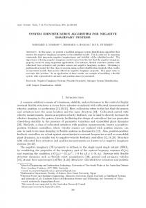
of the ZMNL part are α1 = 14.9740 + 0.0519 j and α3 = −23.0954 + 4.9680 j, which correspond to the parameters of a class AB power amplifier [40]. The input signal√was an i.i.d.√ 8-QAM ª sequence, i.e. drawn from the finite alphabet Λ = {±1 ± j , ±(1 + 3), ±(1 + 3) j , with length N = 16384. An additive, zero-mean, complex, white Gaussian noise was added to the channel output. The simulation results were averaged over 100 independent Monte Carlo runs. The performances were evaluated in terms of Normalized Mean Square Error (NMSE) on the output signal and on the estimated parameters. The third-order Volterra kernel was estimated using the method described in [42].

Figure 8 depicts the convergence behavior of the proposed two-steps ALS algorithm in terms of the estimated parameters of the two linear subsystems and the reconstructed third-order Volterra kernel in the noiseless case. From these simulation results, we can conclude that the two-steps ALS converges fast (about 30 iterations).

5

10

Third−order Volterra kernel First linear subchannel Second linear subchannel

0

10

−5

10

NMSE

−10

10

−15

10

−20

10

−25

10

−30

10

0

20

40 60 Number of iterations

80

100

Fig. 8. ALS convergence for the noiseless LTI-ZMNL-LTI communication channel.

In the noisy case, Figure 9 depicts the NMSE for different SNR values. We can note that the output NMSE corresponds approximately to the noise level, implying that the estimated model well approximates the simulated channel. We also note that the estimation performances of the two LTI subsystems are very close.

34

10 Output First linear subchannel Second linear subchannel ZMNL subchannel

0

NMSE (dB)

−10

−20

−30

−40

−50

−60

0

5

10

15 SNR (dB)

20

25

30

Fig. 9. Output NMSE and parameter NMSE for the estimated LTI-ZMNL-LTI communication channel.

6 Conclusion and future works In this paper, the main definitions and properties relative to tensors have first been recalled before giving a brief review of the most used tensor models. Then, some examples of tensors encountered in SP have been described for signal and system modeling. Finally, some applications of the PARAFAC model have been presented for solving the system identification problem for both linear and nonlinear systems. Tensors constitute a very interesting research area, with very promising applications in various domains. However, fundamental properties of tensors in terms of rank and uniqueness remain to be better understood. New tensor models and tensor decompositions are to be studied, and more robust parameter estimation algorithms are necessary to render tensor-based SP methods even more efficient and attractive. Low-rank approximation of tensors of rank larger than one is also a very important open problem with the objective of tensor dimensionality reduction, which is very useful for tensor object feature extraction and classification. More generally, tensor simplification, like diagonalization for instance, by means of transforms, is also an open issue. Finally, other applications of tensor tools can be considered as, for instance, for multidimensional filtering with application to noise reduction in color images and seismic data [44] and also to channel equalization.

References 1. Hitchcock, F.: The expression of a tensor or a polyadic as a sum of products. J. Math. Phys. Camb. 6 (1927) 164–189 2. Tucker, L.: Some mathematical notes of three-mode factor analysis. Psychometrika 31(3) (1966) 279–311 3. Caroll, J., Chang, J.: Analysis of individual differences in multidimensional scaling via an N-way generalization of "Eckart-Young" decomposition. Psychometrika 35 (1970) 283–319

35 4. Harshman, R.: Foundation of the PARAFAC procedure: models and conditions for an "explanatory" multimodal factor analysis. UCLA working papers in phonetics 16 (1970) 1–84 5. Bro, R.: PARAFAC. Tutorial and applications. Chemometrics and Intelligent Laboratory Systems 38 (1997) 149–171 6. Cardoso, J.F.: Eigen-structure of the fourth-order cumulant tensor with application to the blind source separation problem. In: Proc. Int. Conf. on Acoustics, Speech, and Signal Processing (ICASSP), Albuquerque, New Mexico, USA (3-6 April 1990) 2655–2658 7. Cardoso, J.F.: Super-symmetric decomposition of the fourth-order cumulant tensor. Blind identification of more sources than sensors. In: Proc. Int. Conf. on Acoustics, Speech, and Signal Processing (ICASSP), Toronto, Ontario, Canada, (14-17 May 1991) 3109–3112 8. McCullagh, P.: Tensor methods in statistics. Chapman and Hall (1987) 9. Sidiropoulos, N., Bro, R., Giannakis, G.: Parallel factor analysis in sensor array processing. IEEE Trans. on Signal Processing 48(8) (2000) 2377–2388 10. Sidiropoulos, N., Giannakis, G., Bro, R.: Blind PARAFAC receivers for DS-CDMA systems. IEEE Trans. on Signal Processing 48(3) (March 2000) 810–823 11. de Almeida, A.L.F., Favier, G., Mota, J.C.M.: PARAFAC-based unified tensor modeling for wireless communication systems with application to blind multiuser equalization. Signal Processing 87(2) (February 2007) 337–351 12. Kruskal, J.: Three-way arrays: rank and uniqueness of trilinear decompositions, with application to arithmetic complexity and statistics. Linear Algebra Applicat. 18 (1977) 95–138 13. Sidiropoulos, N., Liu, X.: Identifiability results for blind beamforming in incoherent multipath with small delay spread. IEEE Trans. on Signal Processing 49(1) (Jan. 2001) 228–236 14. Meyer, C.: Matrix analysis and applied linear algebra. SIAM (2000) 15. Eckart, C., Young, G.: The approximation of one matrix by another of lower rank. Psychometrika 1 (1936) 211–218 16. de Almeida, A.L.F., Favier, G., Mota, J.C.M.: Multiuser MIMO system using block spacetime spreading and tensor modeling. Signal Processing 88(10) (October 2008) 2388–2402 17. Comon, P., Golub, G., Lim, L.H., Mourrain, B.: Symmetric tensors and symmetric tensor ranks. SCCM technical report 06-02, Stanford University (2006) 18. Kruskal, J.: Rank, decomposition and uniqueness for 3-way and n-way arrays. In Coppi, R., Bolasco, S., eds.: Multiway data analysis. Elsevier, Amsterdam (1989) 8–18 19. Comon, P., ten Berge, J.: Generic and typical ranks of three-way arrays. Technical report, I3S (Sept. 2006) 20. Kibangou, A., Favier, G.: Blind equalization of nonlinear channels using tensor decompositions with code/space/time diversities. Signal Processing 89(2) (February 2009) 133–143 21. Harshman, R.: Determination and proof of minimum uniqueness conditions for PARAFAC 1. UCLA working papers in phonetics 22 (1972) 111–117 22. ten Berge, J., Sidiropoulos, N.: On uniqueness in CANDECOMP/PARAFAC. Psychometrika 67(3) (2002) 399–409 23. Jiang, T., Sidiropoulos, N.: Kruskal’s permutation lemma and the identification of CANDECOMP/PARAFAC and bilinear models with constant modulus constraints. IEEE Trans. on Signal Processing 52(9) (September 2004) 2625–2636 24. Sidiropoulos, N., Bro, R.: On the uniqueness of multilinear decomposition of n-way arrays. Journal of Chemometrics 14 (2000) 229–239 25. De Lathauwer, L., De Moor, B., Vandevalle, J.: A multilinear singular value decomposition. SIAM J. Matrix Anal. Appl. 21 (April 2000) 1253–1278 26. Kolda, T.: Orthogonal tensor decompositions. SIAM J. Matrix Anal. Appl. 23(1) (2001) 243–255 27. Harshman, R., Lundy, M.: Uniqueness proof for a family of models sharing features of Tucker’s three-mode factor analysis and PARAFAC/CANDECOMP. Psychometrika 61(1) (1996) 133–154

36 28. Kibangou, A., Favier, G.: Blind joint identification and equalization of Wiener-Hammerstein communication channels using PARATUCK-2 tensor decomposition. In: Proc. EUSIPCO, Poznan, Poland (September 2007) 29. de Almeida, A.L.F., Favier, G., Mota, J.C.M.: Space-time spreading-multiplexing for MIMO antenna systems using the PARATUCK2 tensor decomposition. In: Proc. EUSIPCO, Lausanne, Switzerland (August 2008) 30. de Almeida, A.L.F., Favier, G., Mota, J.C.M.: A constrained factor decomposition with application to MIMO antenna systems. IEEE Trans. on Signal Processing 56(6) (June 2008) 2429–2442 31. de Almeida, A.L.F., Favier, G., Mota, J.C.M.: Constrained tensor modeling approach to blind multiple-antenna CDMA schemes. IEEE Trans. on Signal Processing 56(6) (June 2008) 2417–2428 32. Liu, X., Sidiropoulos, N.: Cramer-Rao lower bounds for low-rank decomposition of multidimensional arrays. IEEE Trans. on Signal Processing 49(9) (September 2001) 2074–2086 33. Bro, R.: Multi-way analysis in the food industry. Models, algorithms and applications. PhD thesis, University of Amsterdam, Netherlands (1998) 34. Tomasi, G., Bro, R.: A comparison of algorithms for fitting the PARAFAC model. Comp. Stat. Data Anal. 50(7) (2006) 1700–1734 35. Rajih, M., Comon, P., Harshman, R.: Enhanced line search : a novel method to accelerate PARAFAC. SIAM J. Matrix Anal. (To appear) 36. Fernandes, C.E.R., Favier, G., Mota, J.C.M.: Blind channel identification algorithms based on the PARAFAC decomposition of cumulant tensors: The single and multiuser cases. Signal Processing 88(6) (June 2008) 1382–1401 37. Khouaja, A., Favier, G.: Identification of PARAFAC Volterra cubic models using an alternating recursive least squares algorithm. In: Proc. 12th European Signal Processing Conference (EUSIPCO), Vienna, Austria (September 2004) 1903–1906 38. Kibangou, A., Favier, G.: Matrix and tensor decompositions for identification of blockstructured nonlinear channels in digital transmission systems. In: Proc. IEEE Signal Proc. Advances in Wireless Communications (SPAWC), Recife, Brazil (July 2008) 39. Benedetto, S., Biglieri, E., Daffara, E.: Modeling and performance evaluation of nonlinear satellite links- a Volterra series approach. IEEE Trans. on Aerospace and Electronics Systems 15(4) (July 1979) 494–506 40. Tong Zhou, G., Raich, R.: Spectral analysis of polynomial nonlinearity with applications to RF power amplifiers. EURASIP Journal on Applied Signal Processing 12 (2004) 1831–1840 41. Tseng, C.H., Powers, E.: Identification of nonlinear channels in digital transmission systems. In: Proc. of IEEE Signal Processing Workshop on Higher-order Statistics, South Lake Tahoe, CA (June 1993) 42–45 42. Cheng, C.H., Powers, E.: Optimal Volterra kernel estimation algorithms for a nonlinear communication system for PSK and QAM inputs. IEEE Trans. on Signal Processing 49(1) (2001) 147–163 43. Prakriya, S., Hatzinakos, D.: Blind identification of linear subsystems of LTI-ZMNL-LTI models with cyclostationary inputs. IEEE Trans. on Signal Processing 45(8) (August 1997) 2023–2036 44. Muti, D., Bourennane, S.: Survey on tensor signal algebraic filtering. Signal Processing 87(2) (February 2007) 237–249