Tensor Field Visualisation using Adaptive Filtering of Noise Fields combined with Glyph Rendering Andreas Sigfridsson∗
Tino Ebbers
Einar Heiberg
Lars Wigström
Department of Medicine and Care, Linköpings Universitet, Sweden
A BSTRACT
Methods for visualisation of tensor fields include various generalisations of streamlines to tensor data, such as hyperstreamlines [4]. Their success is highly dependent on starting points, or seeding points. Line integral convolution (LIC), originally a method for visualising vector fields, was introduced by Cabral et al. [2] and further improved by Hege et al. [8]. It is a powerful method that shows direction (or, rather, tangent) of flow in a vector field. One of the advantages of the LIC algorithm is that it has a high spatial resolution. In contrast to the streamline family, no seeding points are needed; LIC visualises the vector field in every point, more or less. The key to the success of LIC is that it creates a continuous representation. To be able to do that, it assumes that the data itself is continuous, and exploits that fact. Mostly, though, physical data has this property, given sufficient resolution. LIC is really designed for vector fields, and not tensor fields. Dickinson [5] suggested that tensors could be visualised as vector fields with the vector being the eigenvector corresponding to the largest eigenvalue. Hsu [9] extended this, suggesting two LIC images to be calculated, one for the largest eigenvalue and one for the next largest eigenvalue, where the image corresponding to the second largest eigenvalue uses a shorter filter length. The images are then added together to form the resulting image. Unfortunately, since the ratio between the eigenvalues is not taken into account, it fails to describe the degree of anisotropy of the tensor field, which is often very useful. Related to LIC is spot noise, introduced by van Wijk [17] and later enhanced by de Leeuw and van Wijk [3]. It can be performed in 3D, but is not adapted to tensor visualisation without modifications. Laidlaw et al. introduced brush strokes as an alternative [13]. This method can convey the degree of anisotropy, but it lacks continuity. Also, it is oriented towards 2D visualisation. A volume rendering approach, designed for 3D diffusion tensors, which shares ideas with the work described in this paper, was proposed by Kindlmann et al. [10]. While being good at visualising diffusion tensors, it is unclear whether it would perform well on strain-rate tensors. It uses a reaction/diffusion method to create a scalar 3D texture, later applied to a shaded surface. This scalar texture has similarities to the scalar overview field we propose, though computed in a different way.
While many methods exist for visualising scalar and vector data, visualisation of tensor data is still troublesome. We present a method for visualising second order tensors in three dimensions using a hybrid between direct volume rendering and glyph rendering. An overview scalar field is created by using three-dimensional adaptive filtering of a scalar field containing noise. The filtering process is controlled by the tensor field to be visualised, creating patterns that characterise the tensor field. By combining direct volume rendering of the scalar field with standard glyph rendering methods for detailed tensor visualisation, a hybrid solution is created. A combined volume and glyph renderer was implemented and tested with both synthetic tensors and strain-rate tensors from the human heart muscle, calculated from phase contrast magnetic resonance image data. A comprehensible result could be obtained, giving both an overview of the tensor field as well as detailed information on individual tensors. CR Categories: I.3.3 [Computer Graphics]: Picture/Image Generation—Viewing algorithms; I.3.8 [Computer Graphics]: Applications; J.2 [Physical Sciences and Engineering]: Engineering; J.3 [Life and Medical Sciences]: Medical Information Systems; Keywords: Tensor, Visualisation, Volume rendering, Glyph rendering, Hybrid rendering, Strain-rate
1
I NTRODUCTION
Visualisation of tensor data has become even more important with the ability to acquire tensor metrics. This can be done with, for example, diffusion tensor magnetic resonance imaging (MRI) [1] or strain-rate calculation from phase-contrast MRI [18, 15, 16]. Add to that the various kinds of simulations that output a tensor field. This paper tries to address some of the problems that arise when visualising symmetric second order tensors in three dimensions.
1.1
Previous Work
One common way of visualising tensors is to represent the tensor with an icon or glyph. The glyph can then represent some or all degrees of freedom from the tensor, depending on it’s type. When visualising tensor fields with one glyph per tensor, it is difficult to make out continuity, because two adjacent glyphs do not form a continuous shape. This gets even more difficult when a 3D tensor field is studied, where occlusion becomes a problem.
2
M ETHODS
We suggest a hybrid visualisation method, consisting of volume rendering of a scalar field for overview visualisation, retaining continuity, and a glyph rendering for detailed tensor analysis with a much smaller region of interest (ROI), showing all degrees of freedom of the tensors while at the same time avoiding occlusion problems. A 3D cursor is then used to position the ROI where the glyph is rendered.
∗ Correspondence to:
[email protected], Department of Medicine and Care, Clinical Physiology, Linköpings Universitet, SE-581 85 Linköping, SWEDEN
IEEE Visualization 2002 Oct. 27 - Nov. 1, 2002, Boston, MA, USA 0-7803-7498-3/02/$17.00 © 2002 IEEE
371
2.1
Scalar Overview Visualisation
For the overview visualisation, the tensor volume is decomposed into a scalar volume, retaining a few, but important, properties of the tensor volume. The scalar volume is created by iterated adaptive filtering of a noise texture, inspired by image enhancement using adaptive filtering, introduced by Knutsson et al. [7, 12]. The noise field is low pass filtered, thereby smearing the noise spots, and then filtered with directed high-pass filters in directions with weak eigenvalues, to cancel out the smearing, leaving spots smeared in strong eigendirections. The result is then visualised using volume rendering techniques, available in different flavours on different hardware for rapid rendering.
2.1.1
Filter Construction
First, one spherically symmetric low-pass filter, Flp , is constructed. Various kinds of low-pass filters can be used, but we chose a Gaussian low pass filter, defined in the frequency domain as 2 − ρ2 2σ
Flp (ρ) = e
(1)
Figure 1: Iso-surface plots of the seven filters in the Fourier domain. The iso-value of the plots is 0.2. The top filter is the low-pass filter Flp , the bottom six filters are the directional high-pass filters Fk .
where ρ is the frequency (with 0 < ρ < π) and σ 2 being the variance of the filter, here empirically set to σ 2 = 0.09. Then, six spherically separable directional high-pass filters are defined. By standard convention, when u is the frequency, ρ = |u| u and u ˆ = |u| . The k-th filter, Fk is defined by its radial component, R(ρ), and directional component, Dk (ˆ u), respectively Fk (u) = R(ρ)Dk (ˆ u)
2.1.2
The tensors are re-mapped to enhance the visual experience. We want to exaggerate the tensor shape to create a more easily recognisable field. If the tensor is closest to being linear (one dominating eigenvalue), we exaggerate it to be even more linear, etc. This is accomplished by re-mapping the eigenvalues and then reconstructing the tensor from the eigenvalues and their respective eigenvectors. First, the eigenvalues are scaled so that the largest eigenvalue, λ1 , becomes 1. The signs of the eigenvalues are discarded, so the scalar overview visualisation does not convey eigenvalue sign. The scaling discards the original norm of the tensors as well. Both of these are visualised using glyph rendering. Then, the eigenvalues are mapped through the function
(2)
The directional part is defined by Dk (ˆ u) = (ˆ nk · u ˆ )2
Tensor Re-mapping
(3)
where n ˆ k is the direction of the filter, defined as the directions of the vertices of an icosahedron: ˆ 1 = c (a, 0, b)T n ˆ 2 = c (−a, 0, b)T n T (4) n ˆ = c (b, a, 0) n ˆ 4 = c (b, −a, 0)T 3 T n ˆ 5 = c (0, b, a) n ˆ 6 = c (0, b, −a)T with
µ(x; α, β) =
a=2 √ b = (1 + 5) √ c = (10 + 2 5)−1/2
(5)
with 1 cos2 Fs (ρ) = 0
π(ρ−ρl ) 2(ρh −ρl )
0 ≤ ρ < ρl ρ l ≤ ρ < ρh ρh ≤ ρ
(7)
which is plotted in Figure 2. The parameters α and β control the shape of the re-mapping function. α is the x where µ crosses 0.5 and β controls the “sharpness” of the function. Higher β means a steeper curve, closer to a step function, lower β gives a function closer to the identity function. We use α = 0.5 and β = 2. The adaptive filtering described by Knutsson et al. [7, 12] is designed for orientation tensors, and will therefore smear across strong eigenvectors instead of along them. Therefore, we re-map the eigenvalues once more so that large eigenvalues become small, and small eigenvalues become large, using the mapping function
These six filters, when combined, are enough to create a filter with any direction, being more computationally efficient compared to creating a new filter for every voxel. This is explained by Knutsson et al. [7, 12] along with the parameter choices for a, b and c. The radial part of the directed high-pass filters are defined as R(ρ) = Fs (ρ) − Flp (ρ)
(|x|(1 − α))β (|x|(1 − α))β + (α(1 − |x|))β
ν(x; α, β) = (6)
2 −1 1 + µ(x; α, β)
(8)
which is in turn plotted in Figure 3.
The Fs is a spherical filter that gives a smooth transition from 1 where ρ < ρl to 0 where ρ > ρh to ensure that the high-pass filter does not pass through any frequencies with ρ > ρh . We have empirically chosen ρl = 0.7π and ρh = π. These filters are created only once, and reused for each iterative step. Iso-surfaces of the seven filters are plotted in Figure 1.
2.1.3
Iterative Filtering
The noise input field, which is a standard Gaussian noise field with a variance of 1, is filtered by multiplication with the filters in the Fourier domain, creating seven filter responses; one low-pass and
372
Remapping function µ(x; α, β)
where I is the 3 by 3 identity matrix, α = 45 and β = 14 in the three-dimensional case, as described by Knutsson et al. [7, 12]. The ck are calculated only once and reused for every iteration. To clarify the algorithm, a two-dimensional example iteration sequence is shown in Figure 4.
2
1.9
1.8
1.7
µ
1.6
1.5
1.4
1.3
1.2
1.1
1
0
0.1
0.2
0.3
0.4
0.5 x
0.6
0.7
0.8
0.9
1
Figure 2: Re-mapping function, µ(x; α, β), attracting eigenvalues to 0 or 1 to exaggerate the shape of the tensor. α = 0.5, β = 2
(a)
(b)
(c)
(d)
Remapping function ν(x; α, β) 1
0.9
0.8
0.7
ν
0.6
0.5
0.4
Figure 4: 2D example of the scalar field showing initial noise image (a), after 3 iterations of adaptive filtering (b), after 6 iterations (c), and after 12 iterations (d).
0.3
0.2
0.1
0
0
0.1
0.2
0.3
0.4
0.5 x
0.6
0.7
0.8
0.9
Since the seven filterings are independent, they were performed in parallel with good speedup using seven processors. Also, most of the filtering time is spent in the Fourier transforms. Since the multidimensional Fourier transforms are separable, they can too be parallelised, if enough processors are available. With large volumes, the memory requirements for the filters and their respective responses are large. Memory requirements were cut in half by exploiting the fact that the filters are real and even in the Fourier domain and the noise field is real in the signal domain. The noise is therefore complex Hermitian in the Fourier domain. Consequently the filter responses are also complex Hermitian in the Fourier domain and thus real in the signal domain.
1
Figure 3: Combined re-mapping function, ν(x; α, β), also mapping low eigenvalues to high and vice versa. α = 0.5, β = 2
six directional high-pass responses. These responses are then recombined to a new image, used as the noise image for the next iteration. The recombination is done by a simple point-by-point weighting of the filter responses s0 = slp +
X
ck sk
2.1.4
The scalar field obtained from the adaptive filtering can be further enhanced by adding colours. One way of adding colour is to encode the eigenvalue distribution, thus showing the degree of anisotropy of the tensor field. This is done with
(9)
k
where slp is low-pass filter response and sk is the filter response from the high-pass filter Fk . The coefficients, ck , are computed for each point as the product sum scalar tensor product ck = C · Mk
λ1 − λ2 λ1 λ2 − λ3 G= λ1 λ3 B= λ1 R=
(10)
where C is the tensor at that point and Mk are the filterassociated dual tensors, defined by Mk = αˆ nk n ˆ Tk − βI
Eigenvalue Distribution Colour Coding
(12) (13) (14)
R, G and B are the components of red, green and blue, respectively. λi are absolute values of the eigenvalues, sorted so that λ1
(11)
373
is the largest. This gives the following properties for R, G and B: 0