To prove termination of Java Bytecode (JBC) automatically, we transform JBC to finite termination graphs which represent all pos- sible runs of the program.
Termination Graphs for Java Bytecode? M. Brockschmidt, C. Otto, C. von Essen, and J. Giesl LuFG Informatik 2, RWTH Aachen University, Germany
Abstract. To prove termination of Java Bytecode (JBC) automatically, we transform JBC to finite termination graphs which represent all possible runs of the program. Afterwards, the graph can be translated into “simple” formalisms like term rewriting and existing tools can be used to prove termination of the resulting term rewrite system (TRS). In this paper we show that termination graphs indeed capture the semantics of JBC correctly. Hence, termination of the TRS resulting from the termination graph implies termination of the original JBC program.
1
Introduction
Termination is an important property of programs. Therefore, techniques to analyze termination automatically have been studied for decades [7, 8, 20]. While most work focused on term rewrite systems or declarative programming languages, recently there have also been many results on termination of imperative programs (e.g., [2, 4, 5]). However, these are “stand-alone” methods which do not allow to re-use the many existing termination techniques and tools for TRSs and declarative languages. Therefore, in [15] we presented the first rewriting-based approach for proving termination of a real imperative object-oriented language, viz. Java Bytecode. Related TRS-based approaches had already proved successful for termination analysis of Haskell and Prolog [10, 16]. JBC [13] is an assembly-like object-oriented language designed as intermediate format for the execution of Java by a Java Virtual Machine (JVM). While there exist several static analysis techniques for JBC, we are only aware of two other automated methods to analyze termination of JBC, implemented in the tools COSTA [1] and Julia [18]. They transform JBC into a constraint logic program by abstracting every object of a dynamic data type to an integer denoting its path-length (i.e., the length of the maximal path of references obtained by following the fields of objects). While this fixed mapping from objects to integers leads to a very efficient analysis, it also restricts the power of these methods. In contrast, in our approach from [15], we represent data objects not by integers, but by terms which express as much information as possible about the data objects. In this way, we can benefit from the fact that rewrite techniques can automatically generate suitable well-founded orders comparing arbitrary forms of terms. Moreover, by using TRSs with built-in integers [9], our approach is not only powerful for algorithms on user-defined data structures, but also for algorithms on pre-defined data types like integers. ?
Supported by the DFG grant GI 274/5-3 and by the G.I.F. grant 966-116.6.
However, it is not easy to transform JBC to a TRS which is suitable for termination analysis. Therefore, we first transform JBC to so-called termination graphs which represent all possible runs of the JBC program. These graphs handle all aspects of the programming language that cannot easily be expressed in term rewriting (e.g., side effects, cyclicity of data objects, object-orientation, etc.). Similar graphs are also used in program optimization techniques [17]. To analyze termination of a set S of desired initial (concrete) program states, we first represent this set by a suitable abstract state. This abstract state is the starting node of the termination graph. Then this state is evaluated symbolically, which leads to its child nodes in the termination graph. This symbolic evaluation is repeated until one reaches states that are instances of states that already appeared earlier in the termination graph. So while we perform considerably less abstraction than direct termination tools like [1, 18], we also apply suitable abstract interpretations [6] in order to obtain finite representations for all possible forms of the heap at a certain program position. Afterwards, a TRS is generated from the termination graph whose termination implies termination of the original JBC program for all initial states S. This TRS can then be handled by existing TRS termination techniques and tools. We implemented this approach in our tool AProVE [11] and in the International Termination Competitions,1 AProVE achieved competitive results compared to Julia and COSTA. So rewriting techniques can indeed be successfully used for termination analysis of imperative object-oriented languages like Java. However, [15] only introduced termination graphs informally and did not prove that these graphs really represent the semantics of JBC. In the present paper, we give a formal justification for the concept of termination graphs. Since the semantics of JBC is not formally specified, in this paper we do not focus on full JBC, but on JINJA Bytecode [12].2 JINJA is a small Java-like programming language with a corresponding bytecode. It exhibits the core features of Java, its semantics is formally specified, and the corresponding correctness proofs were performed in the Isabelle/HOL theorem prover [14]. So in the following, “JBC” always refers to “JINJA Bytecode”. We present the following new contributions: • In Sect. 2, we define termination graphs formally and determine how states in these graphs are evaluated symbolically (Def. 6, 7). To this end, we introduce Eval Ins Ref three kinds of edges in termination graphs ( −→, −→, −→). In contrast to [15], we extend these graphs to handle also method calls and exceptions. • In Sect. 3, we prove that on concrete states, our definition of “symbolic evaluation” is equivalent to evaluation in JBC (Thm. 10). As illustrated in Fig. 1, there is a mapping trans from JBC program states to our notion of concrete states. Then, Thm. 10 proves that if a program state j1 of a jvm JBC program is evaluated to a state j2 (i.e., j1 −→ j2 ), then trans(j1 ) is evaluated to trans(j2 ) using our definitions of “states” and of “symbolic 1 2
See http://www.termination-portal.org/wiki/Termination_Competition. For the same reason, the correctness proof for the termination technique of [18] also regarded a simplified instruction set similar to JINJA instead of full JBC.
Eval
s1 v c1
v SyEv
trans j1
Ins
s2
jvm
v
Ref
s02
s00 2
Eval
c3
trans
j3
}
Thm. 11
}
Thm. 10
...
trans jvm
j2
...
v
v SyEv
c2
s3
...
Fig. 1. Relation between evaluation in JBC and paths in the termination graph SyEv
evaluation” from Sect. 2 (i.e., trans(j1 ) −→ trans(j2 )). • In Sect. 4, we prove that our notion of symbolic evaluation for abstract states correctly simulates the evaluation of concrete states. More precisely, let c1 be a concrete state which can be evaluated to the concrete state c2 (i.e., SyEv
c1 −→ c2 ). Then Thm. 11 states that if the termination graph contains an abstract state s1 which represents c1 (i.e., c1 is an instance of s1 , denoted c1 v s1 ), then there is a path from s1 to another abstract state s2 in the termination graph such that s2 represents c2 (i.e., c2 v s2 ). Note that Thm. 10 and 11 imply the “soundness” of termination graphs, cf. jvm jvm Cor. 12: Suppose there is an infinite JBC-computation j1 −→ j2 −→ . . . where j1 is represented in the termination graph (i.e., there is a state s1 in the termination graph with trans(j1 ) = c1 v s1 ). Then by Thm. 10 there is an infinite symbolic SyEv
SyEv
evaluation c1 −→ c2 −→ . . . , where trans(ji ) = ci for all i. Hence, Thm. 11 implies that there is an infinite so-called computation path in the termination graph starting with the node s1 . As shown in [15, Thm. 3.7], then the TRS resulting from the termination graph is not terminating.
2
Constructing Termination Graphs
To illustrate termination graphs, we regard the method create in Fig. 2. List is a data type whose next field points to the next list element and we omitted the fields for the values of list elements to ease readability. The constructor List(n) creates a new list object with n as its tail. The method create(x) first ensures that x is at least 1. Then it creates a list of length x. In the end, the list is made cyclic by letting the next field of the last list element point to the start of the list. The method create terminates as x is decreased until it is 1. After introducing our notion of states in Sect. 2.1, we describe the construction of termination graphs in Sect. 2.2 and explain the JBC program of Fig. 2 in parallel. Sect. 2.3 formally defines symbolic evaluation and termination graphs. 2.1
States
The nodes of the termination graph are abstract states which represent sets of
public c l a s s L i s t { public L i s t n e x t ; public L i s t ( L i s t n ) { this . next = n ; } public s t a t i c L i s t c r e a t e ( int x ) { List last ; L i s t cur ; i f ( x 2 // call constructor Store " cur " // store into cur Goto " hd " // jump to loop condition
Fig. 2. Java Code and a corresponding JINJA Bytecode for the method create
concrete states, using a formalization which is especially suitable for a translation into TRSs. Our approach is restricted to verified sequential JBC programs without recursion. To simplify the presentation in the paper, as in JINJA, we exclude floating point arithmetic, arrays, and static class fields. However, our approach can easily be extended to such constructs and indeed, our implementation also handles such programs. We define the set of all states as States = (ProgPos × LocVar × OpStack)∗ × ({⊥} ∪ References) × Heap × Annotations . Consider the state in Fig. 3. Its first component is the program position (from ProgPos). In the examples, we represent it by the next program instruction to be executed (e.g., “CmpEq”). Fig. 3. Abstract state The second component are the local variables that have a defined value at the current program position, i.e., LocVar = References∗ . References are addresses in the heap, where we also have null ∈ References. In our representation, we do not store primitive values directly, but indirectly using references to the heap. In examples we denote local variables by names instead of numbers. Thus, “x : i1 , l : o1 , c : o1 ” means that the value of the 0th local variable x is a reference i1 for integers and the 1st and 2nd local variables l and c both reference the address o1 . So different local variables can point to the same address. The third component is the operand stack that JBC instructions operate on, i.e., OpStack = References∗ . The empty operand stack is denoted “ε” and “i2 , i1 ” denotes a stack with top element i2 and bottom element i1 . In contrast to [15], we allow several method calls and a triple from (ProgPos CmpEq | x : i1 , l : o1 , c : o1 | i2 , i1 i1 = [1, ∞) i2 = [1, 1] o1 = List(next = null )
× LocVar × OpStack) is just one frame of the call stack. Thus, an abstract state may contain a sequence of such triples. If a method calls another method, then a new frame is put on top of the call stack. This frame has its own program counter, local variables, and operand stack. Consider the state in Fig. 4, where the List constructor was called. Hence, the top Load "this" | t : o1 , n : null | ε frame on the call stack corresponds to the first Store "cur" | x : i1 | ε statement of this constructor method. The lower i1 = [1, ∞) frame corresponds to the statement Store "cur" o1 = List(next = null ) in the method create. It will be executed when Fig. 4. State with 2 frames the constructor in the top frame has finished. The component from ({⊥} ∪ References) in the definition of States is used for exceptions and will be explained at the end of Sect. 2.2. Here, ⊥ means that no exception was thrown (we omit ⊥ in examples to ease readability). We write the first three components of a state in the first line and separate them by “|”. The fourth component Heap is written in the lines below. It contains information about the values of References. We represent it by a partial function, i.e., Heap = References → Unknown ∪ Integers ∪ Instances. The values in Unknown = Classnames ×{?} represent tree-shaped (and thus acyclic) objects where we have no information except the type. Classnames are the names of all classes and interfaces. For example, “o3 = List(?)” means that the object at address o3 is null or of type List (or a subtype of List). We represent integers as possibly unbounded intervals, i.e. Integers = {{x ∈ Z | a ≤ x ≤ b} | a ∈ Z ∪ {−∞}, b ∈ Z ∪ {∞}, a ≤ b}. So i1 = [1, ∞) means that any positive integer can be at the address i1 . Since current TRS termination tools cannot handle 32-bit int-numbers as in real Java, we treat int as the infinite set of all integers (this is done in JINJA as well). To represent Instances (i.e., objects) of some class, we describe the values of their fields, i.e., Instances = Classnames ×(FieldIDs → References). To prevent ambiguities, in general the FieldIDs also contain the respective class names. So “o1 = List(next = null)” means that at the address o1 , there is a List object and the value of its field next is null. For all (cl , f ) ∈ Instances, the function f is defined for all fields of the class cl and all of its superclasses. All sharing information must be explicitly represented. If an abstract state s contains the non-null references o1 , o2 and does not mention that they could be sharing, then s only represents concrete states where o1 and the references reachable from o1 are disjoint from o2 and the references reachable from o2 . Sharing or aliasing for concrete objects can of course be represented easily, e.g., we could have o2 = List(next = o1 ) which means that o1 and o2 do not point to disjoint parts of the heap h (i.e., they join). But to represent such concepts for unknown objects, we use three kinds of annotations. Annotations are only built for references o 6= null with h(o) ∈ / Integers. Equality annotations like “o1 =? o2 ” mean that the addresses o1 and o2 could be equal. Here the value of at least one of o1 and o2 must be Unknown. To represent states where two objects “may join”, we use joinability annotations “o1 %$ o2 ”. We say that o0 is a direct successor of o in a state s (denoted o →s o0 )
iff the object at address o has a field whose value is o0 . Then “o1 %$ o2 ” means that if the value of o1 is Unknown, then there could be an o with o1 →+ s o and o2 →∗s o, i.e., o is a proper successor of o1 and a (possibly non-proper) successor of o2 . Note that %$ is symmetric,3 so “o1 %$ o2 ” also means that if o2 0 is Unknown, then there could be an o0 with o1 →∗s o0 and o2 →+ s o . Finally, we use cyclicity annotations “o!” to denote that the object at address o is not necessarily tree-shaped (so in particular, it could be cyclic).4 2.2
Termination Graphs, Refinements, and Instances
To build termination graphs, we begin with an abstract state describing all concrete initial states. In our example, we want to know whether all calls of create terminate. So in the corresponding initial abstract state, the value of x is not an actual integer, but (−∞, ∞). After symbolically executing the first JBC instructions, one reaches the instruction “New List”. This corresponds to state A in Fig. 5 where the value of x is from [1, ∞). We can evaluate “New List” without further information about x and reach the node B via an evaluation edge. Here, a new List instance was created at address o1 in the heap and o1 was pushed on the operand stack. “New List” does not execute the constructor yet, but just allocates the needed memory and sets all fields to default values. Thus, the next field of the new object is set to null . “Push null” pushes null on the operand stack. The elements null and o1 on the stack are the arguments for the constructor 2 that is invoked, where “2” means that the constructor with two parameters (n and this) is used. This leads to D, cf. Fig. 4. In the top frame, the local variables this (abbreviated t) and n have the values o1 and null. In the second frame, the arguments that were passed to the constructor were removed from the operand stack. We did not depict the evaluation of the constructor and continue with state E, where the control flow has returned to create. So dotted arrows abbreviate several steps. Our implementation of returns the newly created object as its result. Therefore, o1 has been pushed on the operand stack in E. Evaluation continues to node F , storing o1 in the local variables cur and last (abbreviated c and l). In F one starts with checking the condition of the while loop. To this end, x and the number 1 are pushed on the operand stack and the instruction CmpEq in state G compares them, cf. Fig. 3. We cannot directly continue the symbolic evaluation, because the control flow depends on the value of the number i1 in the variable x. So we refine the information by an appropriate case analysis. This leads to the states H and J where x’s value is from [1, 1] resp. [2, ∞). We call this step integer refinement and G is connected to H and J by refinement edges (denoted by dashed edges in Fig. 5). 3
4
Since both “=? ” and “%$” are symmetric, we do not distinguish between “o1 =? o2 ” and “o2 =? o1 ” and we also do not distinguish between “o1 %$ o2 ” and “o2 %$ o1 ”. It is also possible to use an extended notion of annotations which also include sets of FieldIDs. Then one can express properties like “o may join o0 by using only the field next” or “o may only have a non-tree structure if one uses both fields next and prev” (such annotations can be helpful to analyze algorithms on doubly-linked lists).
... Load "x"| x : i6 , l : o1 , c : o3 | ε i6 = [1, ∞) o1 =? o3 o1 = List(next = null ) o3 = List(?) o1 %$ o3
New List | x : i1 | ε A i1 = [1, ∞) Push null | x : i1 | o1 i1 = [1, ∞) o1 = List(next = null )
B
Invoke | x : i1 | null , o1 i1 = [1, ∞) o1 = List(next = null )
C
Load "this"| t : o1 , n : null | ε Store "cur"| x : i1 | ε i1 = [1, ∞) o1 = List(next = null ) E Store "cur"| x : i1 | o1 i1 = [1, ∞) o1 = List(next = null ) Load "x"| x : i1 , l : o1 , c : o1 | ε i1 = [1, ∞) o1 = List(next = null )
D
O
P
Load "x"| x : i6 , l : o1 , c : o2 | ε i6 = [1, ∞) o1 = List(next = null ) o2 = List(next = o1 )
N
Store "x"| x : i3 ,l : o1 ,c : o1 | i6 i3 = [2, ∞) i6 = [1, ∞) o1 = List(next = null )
M
i6 = i3 + i5 IAdd | x : i3 , l : o1 , c : o1 | i5 ,i3 i3 = [2, ∞) i5 = [−1, −1] o1 = List(next = null ) ...
Load "x"| x : i9 , l : o1 , c : o4 | ε i9 = [1, ∞) o1 =? o3 o1 = List(next = null ) o3 = List(?) o1 %$ o3 o4 = List(next = o3 )
IfFalse | x : i7 , l : o1 , c : o3 | i8 i7 = [1, 1] i8 = [1, 1] o1 =? o3 o1 = List(next = null ) o3 = List(?) o1 %$ o3
Q
L
Putfield | x : i7 ,l : o1 ,c : o3 | o3 ,o1 i7 = [1, 1] o1 =? o3 o1 = List(next = null ) o3 = List(?) o1 %$ o3
Putfield | x : i7 , l : o1 , c : o1 | o1 ,o1 i7 = [1, 1] o1 = List(next = null )
F IfFalse | x : i3 , l : o1 , c : o1 | i4 i3 = [2, ∞) i4 = [0, 0] o1 = List(next = null )
K
CmpEq | x : i1 , l : o1 , c : o1 | i2 ,i1 G CmpEq | x : i3 , l : o1 , c : o1 | i2 ,i3 J i1 = [1, ∞) i2 = [1, 1] i3 = [2, ∞) i2 = [1, 1] o1 = List(next = null ) o1 = List(next = null ) CmpEq | x : i3 , l : o1 , c : o1 | i2 ,i3 H IfFalse | x : i3 , l : o1 , c : o1 | i4 I i3 = [1, 1] i2 = [1, 1] i3 = [1, 1] i4 = [1, 1] o1 = List(next = null ) o1 = List(next = null )
R
S
T Putfield | x : i7 ,l : o1 ,c : o3 | o3 ,o1 i7 = [1, 1] o1 = List(next = null ) o3 = List(?) o1 %$ o3 Load "cur"| x : i7 , l : o1 , c : o3 | ε i7 = [1, 1] o1 = List(next = o3 ) o1 ! o3 ! o3 = List(?) o1 %$ o3 ...
U
...
Fig. 5. Termination graph for create
To define integer refinements, for any s ∈ States, let s[o/o0 ] be the state obtained from s by replacing all occurrences of the reference o in instance fields, the exception component, local variables, and on the operand stacks by o0 . By s+{o 7→ vl } we denote a state which results from s by removing any information about o and instead the heap now maps o to the value vl . So in Fig. 5, J is (G + {i3 7→ [2, ∞)})[i1 /i3 ]. We only keep information on those references in the heap that are reachable from the local variables and the operand stacks. Definition 1 (Integer refinement). Let s ∈ States where h is the heap of s and let o ∈ References with h(o) = V ⊆ Z. Let V1 , . . . , Vn be a partition of V (i.e., V1 ∪. . .∪Vn = V ) with Vi ∈ Integers. Moreover, si = (s+{oi 7→ Vi })[o/oi ] for fresh references oi . Then {s1 , . . . , sn } is an integer refinement of s. In Fig. 5, evaluation of CmpEq continues and we push True resp. False on the operand stack leading to the nodes I and K. To simplify the presentation, in the paper we represent the Booleans True and False by the integers 1 and 0. In I and K, we can then evaluate the IfFalse instruction. From K on, we continue the evaluation by loading the value of x and the constant −1 on the operand stack. In L, IAdd adds the two topmost stack elements. To keep track of this, we create a new reference i6 for the result and label
the edge from L to M by the relation between i6 , i3 , and i5 . Such labels are used when constructing rewrite rules from the termination graph [15]. Then, the value of i6 is stored in x and the rest of the loop is executed. Afterwards in state N , cur points to a list (at address o2 ) where a new element was added in front of the original list at o1 . Then the program jumps back to the instruction Load "x" at the label “hd” in the program, where the loop condition is evaluated. However, evaluation had already reached this instruction in state F . So the new state N is a repetition in the control flow. The difference between F and N is that in F , l and c are the same, while in N , l refers to o1 and c refers to o2 , where the list at o1 is the direct successor (or “tail”) of the list at o2 . To obtain finite termination graphs, whenever the evaluation reaches a program position for the second time, we “merge” the two corresponding states (like F and N ). This widening result is displayed in node O. Here, the annotation “o1 =? o3 ” allows the equality of the references in l and c, as in J. But O also contains “o1 %$ o3 ”. So l may be a successor of c, as in N . We connect N to O by an instance edge (depicted by a thick dashed line), since the concrete states described by N are a subset of the concrete states described by O. Moreover, we could also connect F to O by an instance edge and discard the states G-N which were only needed to obtain the suitably generalized state O. Note that in this way we maintain the essential invariant of termination graphs, viz. that a node “is terminating” whenever all of its children are terminating. To define “instance”, we first define all positions π of references in a state s, where s|π is the reference at position π. A position π is exc or a sequence starting with lvi,j or osi,j for i, j ∈ N (indicating the j th reference in the local variable array or the operand stack of the ith frame), followed by zero or more FieldIDs. Definition 2 (State positions SPos). Let s = (hfr 0 , . . . , fr n i, e, h, a) be a state where each stack frame fr i has the form (ppi , lvi , osi ). Then SPos(s) is the smallest set containing all the following sequences π: • • • •
π = lvi,j where 0 ≤ i ≤ n, lvi = oi,0 , . . . , oi,mi , 0 ≤ j ≤ mi . Then s|π is oi,j . π = osi,j where 0 ≤ i ≤ n, osi = o0i,0 , . . . , o0i,ki , 0 ≤ j ≤ ki . Then s|π is o0i,j . π = exc if e 6= ⊥. Then s|π is e. π = π 0 v for some v ∈ FieldIDs and some π 0 ∈ SPos(s) where h(s|π0 ) = (cl , f ) ∈ Instances and where f (v) is defined. Then s|π is f (v).
For any position π, let π s denote the maximal prefix of π such that π s ∈ SPos(s). We write π if s is clear from the context. In Fig. 5, F |lv0,0 = i1 , F |lv0,1 = F |lv0,2 = o1 . If h is F ’s heap, then h(o1 ) = (List, f ) ∈ Instances, where f (next) = null. So F |lv0,1 next = F |lv0,2 next = null. Intuitively, a state s0 is an instance of a state s if they correspond to the same program position and whenever there is a reference s0 |π , then either the values represented by s0 |π in the heap of s0 are a subset of the values represented by s|π in the heap of s or else, π is no position in s. Moreover, shared parts of the heap in s0 must also be shared in s. Note that since s and s0 correspond to the same position in a verified JBC program, s and s0 have the same number of local variables and their operand stacks have the same size. In Def. 3, the
conditions (a)-(d) handle Integers, null, Unknown, and Instances, whereas the remaining conditions concern equality and annotations. Here, the conditions (e)-(g) handle the case where two positions π, π 0 of s0 are also in SPos(s). Definition 3 (Instance). Let s0 = (hfr 00 , . . . , fr 0n i, e0 , h0 , a0 ) and s = (hfr 0 , . . . , fr n i, e, h, a), where fr 0i = (pp0i , lvi0 , os0i ) and fr i = (ppi , lvi , osi ). We call s0 an instance of s (denoted s0 v s) iff ppi = pp0i for all i and for all π, π 0 ∈ SPos(s0 ): (a) if h0 (s0 |π ) ∈ Integers and π ∈ SPos(s), then h0 (s0 |π ) ⊆ h(s|π ) ∈ Integers. (b) if s0 |π = null and π ∈ SPos(s), then s|π = null or h(s|π ) ∈ Unknown. (c) if h0 (s0 |π ) = (cl 0 , ?) ∈ Unknown and π ∈ SPos(s), then h(s|π ) = (cl , ?) ∈ Unknown and cl 0 is cl or a subtype of cl . (d) if h0 (s0 |π ) = (cl 0 , f 0 ) ∈ Instances and π ∈ SPos(s), then h(s|π ) = (cl , ?) or h(s|π ) = (cl 0 , f ) ∈ Instances, where cl 0 must be cl or a subtype of cl . (e) if s0 |π 6= s0 |π0 and π, π 0 ∈ SPos(s), then s|π 6= s|π0 . (f ) if s0 |π = s0 |π0 and π, π 0 ∈ SPos(s) where h0 (s0 |π ) ∈ Instances ∪ Unknown, then s|π = s|π0 or s|π =? s|π0 .5 (g) if s0 |π =? s0 |π0 and π, π 0 ∈ SPos(s), then s|π =? s|π0 . � (h) if s0 |π = s0 |π0 or s0 |π =? s0 |π0 where h0 (s0 |π ) ∈ Instances ∪ Unknown and {π, π 0 } 6⊆ SPos(s) with π 6= π 0 , then s|π %$ s|π0 . (i) if s0 |π %$ s0 |π0 , then s|π %$ s|π0 . (j) if s0 |π ! holds, then s|π !. (k) if there exist ρ, ρ0 ∈ FieldIDs∗ without common prefix where ρ 6= ρ0 , s0 |πρ = s0 |πρ0 , h0 (s0 |πρ ) ∈ Instances ∪ Unknown, and ( {πρ, πρ0 } 6⊆ SPos(s) or s|πρ =? s|πρ0 ), then s|π !. In Fig. 5, we have F v O and N v O. Symbolic evaluation can continue in the new generalized state O. It again leads to a node like G, where an integer refinement is needed to continue. If the value in x is still not 1, eventually one has to evaluate the loop condition again (in node P ). Since P v O, we draw an instance edge from P to O and can “close” this part of the termination graph.6 If the value in x is 1 (which is checked in state Q), we reach state R. Here, the references o1 and o3 in l and c have been loaded on the operand stack and one now has to execute the Putfield instruction which sets the next field of the object at the address o1 to o3 . To find out which references are affected by this operation, we need to decide whether o1 = o3 holds. To this end, we perform an equality refinement according to the annotation “o1 =? o3 ”. Definition 4 (Equality refinement). Let s ∈ States where h is the heap of s and where s contains “o =? o0 ”. Hence, h(o) ∈ Unknown or h(o0 ) ∈ Unknown. 5
6
For annotations concerning s|π with π ∈ SPos(s), we usually do not mention that they are from the Annotations component of s, since s is clear from the context. If P had not been an instance of O, we would have performed another widening step and created a new node which is more general than O and P . By a suitably aggressive widening strategy, one can ensure that after finitely many widening steps, one always reaches a “fixpoint”. Then all states that result from further symbolic evaluation are instances of states that already occurred earlier. In this way, we can automatically generate a finite termination graph for any non-recursive JBC program.
W.l.o.g. let h(o) ∈ Unknown. Let s= = s[o/o0 ] and let s6= result from s by removing “o =? o0 ”. Then {s= , s6= } is an equality refinement of s. In Fig. 5, equality refinement of R results in S (where o1 = o3 ) and T (where o1 6= o3 and thus, “o1 =? o3 ” was removed). In T ’s successor U , the next field of o1 has been set to o3 . However, o1 and o3 may join due to “o1 %$ o3 ”. So in particular, T also represents states where o3 →+ o1 . Thus, writing o3 to a field of o1 could create a cyclic data object. Therefore, all non-concrete elements in the abstracted object must be annotated with !. Consequently, our symbolic evaluation has to extend our state with “o1 !” and “o3 !”. From U on, the graph construction can be finished directly by evaluating the remaining instructions. From the termination graph, one could generate the following 1-rule TRS which describes the operations on the cycle of the termination graph. fO (i6 , List(null), o3 ) → fO (i6 − 1, List(null), List(o3 )) | i6 > 0 ∧ i6 6= 1
(1)
Here we also took the condition from the states before O into account which ensures that the loop is only executed for numbers x that are greater than 0. As mentioned in Sect. 1, we regard TRSs where the integers and operations like “−”, “>”, “6=” are built in [9] and we represent objects by terms. So essentially, for any class C with n fields we introduce an n-ary function symbol C whose arguments correspond to the fields of C. Hence, the object List(next = null) is represented by the term List(null). A state like O is translated into a term fO (. . .) whose direct subterms correspond to the exception component (if it is not ⊥), the local variables, and the entries of the operand stack. Hence, Rule (1) describes that in each loop iteration, the value of the 0th local variable decreases from i6 to i6 − 1, the value of the 1st variable remains List(null), and the value of the 2nd variable increases from o3 to List(o3 ). Termination of this TRS is easy to show and indeed, AProVE proves termination of create automatically. Finally, we have a third kind A Getfield | x : o1 | o1 Getfield | x : null | null of refinement. This instance reo1 = List(?) o1 ! C finement is used if we need inh i exception: o2 E formation about the existence or Getfield | x : o2 | o2 o2 = NullPointer() B the type of an Unknown instance. o2 = List(next = o3 ) D o3 = List(?) o2 ! o3 ! Consider Fig. 6, where in state A Getfield | x : o1 | o1 o2 %$ o3 o2 =? o3 o1 = List(next = o1 ) we want to access the next field of ... the List object in o1 . However, we Fig. 6. Instance refinement and exceptions cannot evaluate Getfield, as the instance in o1 is Unknown. To refine o1 , we create a successor B where the instance exists and is exactly of type List and a state C where o1 is null. In A the instance may be cyclic, indicated by o1 !. For this reason, the instance refinement has to add appropriate annotations to B. For example, state D (where o1 is a concrete cyclic list) is an instance of B. In C, evaluation of Getfield throws a NullPointer exception. If an exception handler for this type is defined, evaluation would continue there and a reference to the NullPointer object is pushed to the operand stack. But here, no such handler exists and E reaches a program end. Here, the call stack is empty and
the exception component e is no longer ⊥, but an object o2 of type NullPointer. Definition 5 (Instance refinement). Let s ∈ States where h is the heap of s and h(o) = (cl , ?). Let cl 1 , . . . , cl n be all non-abstract (not necessarily proper) subtypes of cl . Then {snull , s1 , . . . , sn } is an instance refinement of s. Here, snull = s[o/ null ] and in si , we replace o by a fresh reference oi pointing to an object of type cl i . For all fields vi,1 . . . vi,mi of cl i (where vi,j has type cl i,j ), a new reference oi,j is generated which points to the most general value vl i,j of type cl i,j , i.e., (−∞, ∞) for integers and cl i,j (?) for reference types. Then si is (s + {oi 7→ (cl i , fi ), oi,1 7→ vl i,1 , . . . , oi,mi 7→ vl i,mi })[o/oi ], where fi (vi,j ) = oi,j for all j. Moreover, new annotations are added in si : If s contained o0 %$ o, we add o0 =? oi,j and o0 %$ oi,j for all j.7 If we had o!, we also add oi,j !, oi =? oi,j , oi %$ oi,j , oi,j =? oi,j 0 , and oi,j %$ oi,j 0 for all j, j 0 with j 6= j 0 . 2.3
Defining Symbolic Evaluation and Termination Graphs
To define symbolic evaluation formally, for every JINJA instruction, we formulate a corresponding inference rule for symbolic evaluation of our abstract states. This is straightforward for all JINJA instructions except Putfield. Thus, in Def. 6 we only present the rules corresponding to a simple JINJA Bytecode instruction (Load) and to Putfield. We will show in Sect. 3 that on non-abstract states, our inference rules indeed simulate the semantics of JINJA. For a state s whose topmost frame has m local variables with values o0 , . . . , om , “Load b” pushes the value ob of the bth local variable to the operand stack. Executing “Putfield v” in a state with the operand stack o0 , o1 , . . . , ok means that one wants to write o0 to the field v of the object at address o1 . This is only allowed if there is no annotation “o1 =? o” for any o. Then the function f that maps every field of o1 to its value is updated such that v is now mapped to o0 . However, we may also have to c s Putfield | . . . | o0 , o1 Putfield | . . . | o0 , o1 update annotations when evaluatp = List(next = o1 ) p = List(?) p %$ o1 v o1 = List(next = null) o1 = List(next = null) ing Putfield. Consider the cono0 = List(?) o0 = List(next = null) crete state c and the abstract 0 0 state s in Fig. 7. We have c v s, as ... | ... | ε c s ... | ... | ε p = List(?) p %$ o1 p = List(next = o1 ) the connection between p and o1 v o1 = List(next = o0 ) o1 = List(next = o0 ) in c (i.e., p →∗c o1 ) was replaced o0 = List(?) p %$ o0 o0 = List(next = null) by “p %$ o1 ” in s. In both states, Fig. 7. Putfield and annotations we consider a Putfield instruction which writes o0 into the field next of o1 . For c, we obtain the state c0 where we we now also have p →∗c0 o0 . However, to evaluate Putfield in the abstract state s, it is not sufficient to just write o0 to the field next of o1 . Then c0 would not be an instance of the resulting state s0 , since s0 would not represent the connection between p and o0 . Therefore, we have to add “p %$ o0 ” in s0 . Now c0 v s0 indeed holds. A similar problem was discussed for node U of Fig. 5, where we had to add “!” annotations after evaluating Putfield. 7
Of course, if cl i,j and the type of o0 have no common subtype or one of them is int, then o0 =? oi,j does not need to be added.
To specify when we need such additional annotations, for any state s let o ∼s o0 denote that “o =? o0 ” or “o %$ o0 ” is contained in s. Then we define s as →∗s ◦ (= ∪ ∼s ), i.e., o s o00 iff there is an o0 with o →∗s o0 , where o0 = o00 or o0 ∼s o00 . We drop the index “s” if s is clear from the context. For example, in Fig. 7, we have p →∗c0 o1 , p →∗c0 o0 and p s0 o1 , p s0 o0 . Consider a Putfield instruction which writes the reference o0 into the instance referenced by o1 . After evaluation, o1 may reach any reference q that could be reached by o0 up to now. Moreover, q cannot only be reached from o1 , but from every reference p that could possibly reach o1 up to now. Therefore, we must add “p %$ q” for all p, q with p ∼ o1 and o0 q. Moreover, Putfield may create new non-tree shaped objects if there is a reference p that can reach a reference q in several ways after the evaluation. This can only happen if p q and p o1 held before (otherwise p would not be influenced by Putfield). If the new field content o0 could also reach q (o0 q), a second connection from p over o0 to q may be created by the evaluation. Then we have to add “p!” for all p for which a q exists such that p q, p o1 , and o0 q.8 It suffices to do this for references p where the paths from p to o1 and from p to q do not have a common non-empty prefix. Finally, o0 could have reached a non-tree shaped object or a reference q marked with !. In this case, we have to add “p!” for all p with p ∼ o1 . In Def. 6, for any mapping h, let h + {k 7→ d} be the function that maps k to d and every k 0 6= k to h(k 0 ). For pp ∈ ProgPos, let pp + 1 be the position of the next instruction. Moreover, instr (pp) is the instruction at position pp. SyEv
Definition 6 (Symbolic evaluation −→ ). For every JINJA instruction, we define a corresponding inference rule for symbolic evaluation of states. We write SyEv s −→ s0 if s is transformed to s0 by one of these rules. Below, we give the rules for Load and Putfield (in the case where no exception was thrown). The rules for the other instructions are analogous. s = (h(pp, lv, os), fr 1 , . . . , fr n i, ⊥, h, a) instr (pp) = Load b lv = o0 , . . . , om os = o00 , . . . , o0k s0 = (h(pp + 1, lv, os0 ), fr 1 , . . . , fr n i, ⊥, h, a) os0 = ob , o00 , . . . , o0k s = (h(pp, lv, os), fr 1 , . . . , fr n i, ⊥, h, a) instr(pp) = Putfield v os = o0 , o1 , o2 , . . . , ok h(o1 ) = (cl , f ) ∈ Instances a contains no annotation o1 =? o s0 = (h(pp + 1, lv, os0 ), fr 1 , . . . , fr n i, ⊥, h0 , a0 ) os0 = o2 , . . . , ok 0 0 0 h = h + (o1 7→ (cl , f )) f = f + (v 7→ o0 ) 0 In the rule for Putfield, a contains all annotations in a, and in addition: • a0 contains “p %$ q” for all p, q with p ∼s o1 and o0 s q • a0 contains “p!” for all p where p s q, p s o1 , o0 s q for some q, and where the paths from p to o1 and p to q have no common non-empty prefix. 8
This happened in state T of Fig. 5 where o3 was written to the field of o1 . We already had o1 T o3 and o3 T o1 , since T contained the annotation “o1 %$ o3 ”. Hence, in the successor state U of T , we had to add the annotations “o1 !” and “o3 !”.
• if a contains “q!” for some q with o0 →∗s q or if there are π, ρ, ρ0 with ρ 6= ρ0 where s|π = o0 and s|πρ = s|πρ0 , then a0 contains “p!” for all p with p ∼s o1 . Finally, we define termination graphs formally. As illustrated, termination graphs are constructed by repeatedly expanding those leaves that do not correspond to program ends (i.e., where the call stack is not empty). Whenever possible, we evaluate the abstract state in a leaf (resulting in an evaluation edge Eval −→ ). If evaluation is not possible, we use a refinement to perform a case analysis Ref (resulting in refinement edges −→ ). To obtain a finite graph, we introduce more general states whenever a program position is visited a second time in our symIns bolic evaluation and add appropriate instance edges −→ . However, we require all cycles of the termination graph to contain at least one evaluation edge. Definition 7 (Termination graph). A graph (N, E) with N ⊆ States and E ⊆ N × {Eval, Ref, Ins} × N is a termination graph if every cycle contains at least one edge labelled with Eval and one of the following holds for each s ∈ N : SyEv
• s has just one outgoing edge (s, Eval, s0 ) and s −→ s0 . • There is a refinement {s1 , . . . , sn } of s according to Def. 1, 4, or 5, and the outgoing edges of s are (s, Ref, s1 ), . . . , (s, Ref, sn ). • s has just one outgoing edge (s, Ins, s0 ) and s v s0 . • s has no outgoing edge and s = (ε, e, h, a).
3
Simulating JBC by Concrete States
In this section we show that if one only regards concrete states, the rules for symbolic evaluation in Def. 6 correspond to the operational semantics of JINJA. Definition 8 (Concrete states). Let c ∈ States and let h be the heap of c. We call c concrete iff c contains no annotations and for all π ∈ SPos(c), either c|π = null or h(c|π ) ∈ Instances ∪ {[z, z] | z ∈ Z}. Def. 9 recapitulates the definition of JINJA states from [12] in a formulation that is similar to our states. However, integers are not represented by references, there are no integer intervals, no unknown values, and no annotations. Definition 9 (JINJA states). Let Val = Z ∪ References. Then we define: (ProgPos × JinjaLocVar × JinjaOpStack)∗ × ({⊥} ∪ References) × JinjaHeap JinjaLocVar = Val∗ JinjaOpStack = Val∗ JinjaHeap = References → JinjaInstances JinjaInstances = Classnames ×(FieldIDs → Val)
JinjaStates =
To define a function trans which maps each JINJA state to a corresponding concrete state, we first introduce a function tr Val : Val → References with tr Val (o) = o for all o ∈ References. Moreover, tr Val maps every z ∈ Z to a fresh reference oz . Later, the value of oz in the heap will be the interval [z, z]. Now we define tr Ins : JinjaInstances → Instances. For any f : FieldIDs
→ Val, let tr Ins (cl , f ) = (cl , fe), where fe(v) = tr Val (f (v)) for all v ∈ FieldIDs. Next we define tr Heap : JinjaHeap → Heap. For any h ∈ JinjaHeap, tr Heap (h) is a function from References to Integers ∪ Instances. For any o ∈ References, let tr Heap (h)(o) = tr Ins (h(o)). Furthermore, we need to add the new references for integers, i.e., tr Heap (h)(oz ) = [z, z] for all z ∈ Z. Let tr Frame : (ProgPos × JinjaLocVar × JinjaOpStack) → (ProgPos e os). × LocVar × OpStack) with tr Frame (pp, lv, os) = (pp, lv, e If lv = o0 , . . . , om , 0 0 e e = tr Val (o00 ), . . . , tr Val (o0k ). os = o0 , . . . , ok , then lv = tr Val (o0 ), . . . , tr Val (om ), os Finally we define trans : JinjaStates → States. For any j ∈ JinjaStates with j = (hfr 0 , . . . , fr n i, e, h), let trans(j) = (htr Frame (fr 0 ), . . . , tr Frame (fr n )i, e0 , tr Heap (h), ∅), where e0 = ⊥ if e = ⊥ and e0 = tr Val (e) otherwise. jvm
For j, j 0 ∈ JinjaStates, j −→ j 0 denotes that evaluating j one step accordjvm ing to the semantics of JINJA [12] leads to j 0 . Thm. 10 shows that −→ can be simulated by the evaluation of concrete states as defined in Def. 6, cf. Fig. 1. Theorem 10 (Evaluation of concrete states simulates JINJA evaluajvm
SyEv
tion). For all j, j 0 ∈ JinjaStates, j −→ j 0 implies trans(j) −→ trans(j 0 ). Proof. We give the proof for the most complex JINJA instruction (i.e., Putfield in the case where no exception was thrown). The proof is analogous for the other jvm
instructions. Here, −→ is defined by the following inference rule. j = (h(pp, lv, os), fr 1 , . . . , fr n i, ⊥, h) instr(pp) = Putfield v os = o0 , o1 , o2 , . . . , ok h(o1 ) = (cl , f ) ∈ JinjaInstances j 0 = (h(pp + 1, lv, os0 ), fr 1 , . . . , fr n i, ⊥, h0 ) os0 = o2 , . . . , ok 0 0 0 h = h + (o1 7→ (cl , f )) f = f + (v 7→ o0 ) jvm
e os), Let j −→ j 0 by the above rule. Then trans(j) = (h(pp, lv, e tr Frame (fr 1 ), . . . , tr Frame (fr n )i, ⊥, tr Heap (h), ∅) with os e = tr Val (o0 ), tr Val (o1 ), . . . , tr Val (ok ). e os f0 ), tr Frame (fr 1 ), Note that tr Val (o1 ) = o1 . Moreover, trans(j 0 ) = (h(pp + 1, lv, 0 0 f = tr Val (o2 ), . . . , tr Val (ok ). . . . , tr Frame (fr n )i, ⊥, tr Heap (h ), ∅) with os SyEv
On the other hand, by Def. 6 for c = trans(j), we have c −→ c0 with c0 = e os f0 ), tr Frame (fr 1 ), . . . , tr Frame (fr n )i, ⊥, tr Heap (h)0 , ∅). It remains to (h(pp + 1, lv, show that tr Heap (h0 ) = tr Heap (h)0 . For any new reference oz for integers, we have tr Heap (h0 )(oz ) = [z, z] = tr Heap (h)0 (oz ). For any o ∈ References \{o1 }, we have tr Heap (h0 )(o) = tr Ins (h0 (o)) = tr Ins (h(o)) and tr Heap (h)0 (o) = tr Heap (h)(o) = tr Ins (h(o)). Finally, tr Heap (h0 )(o1 ) = tr Ins (h0 (o1 )) = tr Ins (cl , f 0 ) = (cl , fe0 ) where fe0 (v) = tr Val (o0 ) and fe0 (w) = tr Val (f (w)) for all w ∈ FieldIDs \{v}. Moreover, tr Heap (h)0 (o1 ) = (cl , (fe)0 ) where (fe)0 (v) = tr Val (o0 ) and (fe)0 (w) = fe(w) = tr Val (f (w)) for all w ∈ FieldIDs \{v}. t u
4
Simulating Concrete States by Abstract States
Now we show that our symbolic evaluation on abstract states is indeed consistent with the evaluation of all represented concrete states, cf. the upper half of Fig. 1.
Theorem 11 (Evaluation of abstract states simulates evaluation of conSyEv
crete states). Let c, c0 , s ∈ States, where c is concrete, c −→ c0 , c v s, and Ins Ref s occurs in a termination graph G. Then G contains a path s(−→ ∪ −→)∗ Eval ◦ −→ s0 such that c0 v s0 . Proof. We prove the theorem by induction on the sum of the lengths of all paths Eval from s to the next −→ edge. This sum is always finite, since every cycle of a termination graph contains an evaluation edge, cf. Def. 7. We perform a case Ins analysis on the type of the outgoing edges of s. If there is an edge s −→ s˜, and hence s v s˜, we prove transitivity of v (Lemma 13, Sect. 4.1). Then c v s implies c v s˜ and the claim follows from the induction hypothesis. Ref Ref Ref If the outgoing edges of s are −→ edges (i.e., s −→ s1 , . . . , s −→ sn ), we show that our refinements are “valid ”, i.e., c v s implies c v sj for some sj (Lemmas 14-16, Sect. 4.2). Again, then the claim follows from the induction hypothesis. SyEv
Eval
Finally, if the first step is an −→-step (i.e., s −→ s0 ), we prove the correctSyEv
ness of the −→ relation on abstract states (Lemma 19, Sect. 4.3).
t u
With Thm. 10 and 11, we can prove the “soundness” of termination graphs. Corollary 12 (Soundness of termination graphs). Let j1 ∈ JinjaStates jvm
jvm
have an infinite evaluation j1 −→ j2 −→ . . . and let G be a termination graph with a state s11 such that trans(j1 ) v s11 . Then G contains an infinite computation path s11 , . . . , sn1 1 , s12 , . . . , sn2 2 , . . . such that trans(ji ) v s1i for all i. Proof. The corollary follows directly from Thm. 10 and 11, cf. Sect. 1.
t u
As shown in [15, Thm. 3.7], if the TRS resulting from a termination graph is terminating, then there is no infinite computation path. Thus, Cor. 12 proves the soundness of our approach for automated termination analysis of JBC. 4.1
Transitivity of v
Lemma 13 (v transitive). If s00 v s0 and s0 v s, then also s00 v s. Proof. We prove the lemma by checking each of the conditions in Def. 3. Here, we only consider Def. 3(a)-(d) and refer to [3] for the (similar) proof of the remaining conditions. Let π ∈ SPos(s) and let h (h0 , h00 ) be the heap of s (s0 , s00 ). Note that π ∈ SPos(s) implies π ∈ SPos(s0 ) and π ∈ SPos(s00 ), cf. [15, Lemma 4.1]. (a) If h00 (s00 |π ) ∈ Integers, then because of s00 v s0 also h0 (s0 |π ) ∈ Integers and thus h(s|π ) ∈ Integers. We also have h00 (s00 |π ) ⊆ h0 (s0 |π ) ⊆ h(s|π ). (b) If s00 |π = null , then by s00 v s0 we have either s0 |π = null and thus, s|π = null or h(s|π ) ∈ Unknown or h0 (s0 |π ) ∈ Unknown and thus, h(s|π ) ∈ Unknown. (c) If h00 (s00 |π ) = (cl 00 , ?), then h0 (s0 |π ) = (cl 0 , ?) and thus also h(s|π ) = (cl , ?). Here, cl 00 is cl 0 or a subtype of cl 0 , and cl 0 is cl or a subtype of cl . Note that the subtype relation of JBC types is transitive by definition. (d) If h00 (s00 |π ) = (cl 00 , f 00 ) ∈ Instances, then either
h0 (s0 |π ) = (cl 0 , ?) and thus, also h(s|π ) = (cl , ?) or h0 (s0 |π ) = (cl 00 , f 0 ) ∈ Instances and thus, either h(s|π ) = (cl , ?) or h(s|π ) = (cl 00 , f ) ∈ Instances. Again, cl 00 is cl 0 or a subtype of cl 0 , and cl 0 is cl or a subtype of cl . 4.2
t u
Validity of refinements
We say that a refinement ρ : States → 2States is valid iff for all s ∈ States and all concrete states c, c v s implies that there is an s0 ∈ ρ(s) such that c v s0 . We now prove the validity of our refinements from Def. 1, 4, and 5. Lemma 14. The integer refinement is valid. Proof. Let {s1 , . . . , sn } be an integer refinement of s where si = (s + {oi 7→ Vi })[o/oi ] and hs (o) = V = V1 ∪ . . . ∪ Vn ⊆ Z for the heap hs of s. Let c be a concrete state with heap hc and c v s. Let Π = {π ∈ SPos(s) | s|π = o}. By Def. 3(e), there is a z ∈ Z such that hc (c|π ) = [z, z] for all π ∈ Π. Let z ∈ Vi and let hsi be the heap of si . Then hsi (si |π ) = Vi for all π ∈ Π. To show c v si , we only have to check condition Def. 3(a). Let τ ∈ SPos(c) ∩ SPos(si ) with hc (c|τ ) = [z 0 , z 0 ] ∈ Integers. If τ 6∈ Π, then this position was not affected by the integer refinement and thus, hc (c|τ ) ⊆ hs (s|τ ) = hsi (si |τ ). If τ ∈ Π, then we have z 0 = z and thus hc (c|τ ) ⊆ Vi = hsi (si |τ ). t u Lemma 15. The equality refinement is valid. Proof. Let {s= , s6= } be an equality refinement of s, using the annotation o =? o0 . Let c be a concrete state with c v s. We want to prove that c v s6= or c v s= . Let Π = {τ ∈ SPos(s) | s|τ = o}, Π 0 = {τ 0 ∈ SPos(s) | s|τ 0 = o0 }. By Def. 3(e) there are oc and o0c with c|τ = oc for all τ ∈ Π and c|τ 0 = o0c for all τ 0 ∈ Π 0 . If oc 6= o0c , we trivially have c v s6= , as s6= differs from s only in the removed annotation “o =? o0 ” which is not needed when regarding instances like c. s= s If oc = o0c , we prove c v s= . The τ τ0 only change between s and s= was τ τ0 β η η on or below positions in Π. Consider 0 0 o β o o Fig. 8, where a state s with s|τ = o Fig. 8. Illustrating Lemma 15 and s|τ 0 = o0 is depicted on the left 0 0 (i.e., τ ∈ Π and τ ∈ Π ). When we perform an equality refinement and replace o by o0 , we reach the state s= on the right. As illustrated there, we can decompose any position π ∈ SPos(s= ) with a prefix in Π into τ βη, where τ is the shortest prefix in Π and τ β is the longest prefix with s= |τ β = s= |τ . With this decomposition, we have s= |τ = s|τ 0 for τ 0 ∈ Π 0 and thus s= |τ βη = s= |τ η = s= |τ 0 η = s|τ 0 η . For c v s= , we now only have to check the conditions of Def. 3 for any position of s= of the form τ βη as above. Then the claim follows directly, as the conditions of Def. 3 already hold for τ 0 η, since c v s. t u Lemma 16. The instance refinement is valid. Proof. Let S = {snull , s1 , . . . , sn } be an instance refinement of s on reference o. Let c be concrete with heap hc and c v s. We prove that c v s0 for some s0 ∈ S.
By Def. 5, hs (o) = (cl , ?), where hs is the heap of s. Let Π = {π ∈ SPos(s) | s|π = o}. The instance refinement only changed values at positions in Π and below. It may have added annotations for references at other positions, but as annotations only allow more sharing effects, we do not have to consider these positions. By Def. 3(e), there is an oc such that c|π = oc for all π ∈ Π. If oc = null , we set s0 = snull . If hc (oc ) = (cl i , f ), we set s0 = si , where si is obtained by refining the type cl to cl i . Now one can prove c v s0 by checking all conditions of Def. 3, as in the proof of Lemma 13. For the full proof, see [3]. t u 4.3
Correctness of symbolic evaluation
Finally, we prove that every evaluation of a concrete state is also represented by the evaluation of the corresponding abstract state. This is trivial for most instructions, since they only affect the values of local variables or the operand stack. The only instruction which changes data objects on the heap is Putfield. Consider the evaluation of a concrete state c c0 to another state c0 by executing “Putfield v” τ η v which writes o0 to the field v of the object at ado1 o0 dress o1 . Similar to the proof of Lemma 15, evα ery position π of c0 where the state was changed Fig. 9. Illustrating Lemma 17 can be decomposed into π = τ βη. Here, the first part τ leads to o1 and it is the longest prefix that is not affected by the evaluation of Putfield. Similarly, the last part η is the longest suffix of π that was not changed by evaluating Putfield. So in particular, c0 |τ β = o0 . The middle part β contains those parts that were actually changed in the evaluation step. So usually, β is just the field v. However, if o0 →∗c o1 , then the object at o1 in c0 has become cyclic and then β can be more complex. Consider Fig. 9, where c0 |τ = o1 and regard the position π = τ v α v η. Here, the position π was influenced twice by the evaluation, as the middle part β = v α v contains a cycle using the field v. In the following, let π1 < π2 denote that π1 is a proper prefix of π2 and let ≤ be the reflexive closure of