Texture Classification Using Joint Statistical ... - IEEE Xplore

Texture Classification Using Joint Statistical Representation in Space-frequency Domain with Local Quantized Patterns ∗ Institute

Tiecheng Song∗ , Hongliang Li∗ , Bing Zeng∗† and Moncef Gabbouj‡

of Image Processing, University of Electronic Science and Technology of China, Chengdu 611731, China † Department of Electronic and Computer Engineering, The Hong Kong University of Science and Technology, Clearwater Bay, Kowloon, Hong Kong ‡ Department of Signal Processing, Tampere University of Technology, P.O. Box 553, FIN-33101 Tampere, Finland

Abstract—Despite its success in texture analysis, Local Binary Pattern (LBP) is operated in the original image space, and it fails to capture deeper pixel interactions to provide a more discriminative description. In this paper, we propose to explore the joint statistical representation in the space-frequency domain with local quantized patterns for texture classification. The proposed method consists of two channels. In each channel, the multi-resolution spatial filters are employed to generate multiscale spatial maps and the local Fourier transform is subsequently applied to extract local frequency features (spectral maps). The global thresholding is adopted to quantize the spatial and spectral maps into different levels, which are then jointly encoded to built a space-frequency co-occurrence histogram. Finally, the two-channel feature histograms are combined to represent the texture. Experiments on the Outex texture database demonstrate the robustness of our method to image rotation and illumination changes, and our method outperforms the state of the art in terms of the classification accuracy.

I. I NTRODUCTION Feature extraction from images serves as a basic building block in a variety of computer vision applications including image matching [1], texture retrieval [2] and visual classification [3]. In the past few decades, many approaches have been proposed for texture analysis. Because of the computational simplicity and robustness to illumination and rotation changes, Local Binary Pattern (LBP) [4] has received increasing attention in texture classification and face recognition. A lot of variants of LBP have been proposed. To improve the robustness to noise in near-flat regions, Local Ternary Pattern (LTP) [5] was proposed to quantize the local differences into three levels with a fixed threshold. To extract discriminative patterns, Dominant LBP (DLBP) [6] was presented to select the most frequently occurring patterns as features. To be robust to image noise, Dominant Neighborhood Structure (DNS) [7] was developed to combine local and global features to improve the classification performance. In [8], Completed LBP (CLBP) was developed to extract three complementary features: the local difference sign and magnitude components as well as the center pixel. Furthermore, the global thresholding was used in CLBP to quantize local difference magnitudes and the center pixel into two levels. Recently, Local Binary Count (LBC) [9] was introduced to tackle the image rotation by defining the

978-1-4799-3432-4/14/$31.00 ©2014 IEEE

pixel code as the number of bit 1 in the corresponding binary string. Following the CLBP, the Completed LBC (CLBC) was also defined in [9]. One shortcoming of CLBP and CLBC is that they suffer from the high feature dimensionality when considering long-range pixel interactions. In addition, [10]– [12] utilized the circular neighbourhoods like the neighbour sampling in LBP, and then applied the Fourier transform to obtain rotation invariant frequency features. Despite its success, LBP is operated in the original image space, and it lacks deeper pixel interactions in different feature domains. In this paper, we propose to explore the joint statistical representation in the space-frequency domain with local quantized patterns for texture classification. The multi-resolution spatial filters are adopted to capture multiscale image structures. Then, the locally invariant frequency features are extracted and quantized into several levels via global threshoding. Finally, the joint statistical representation in the space-frequency domain is explored to capture a richer description. Since the extracted space-frequency features are robust to image rotation and illumination changes and the deeper pixel interactions are considered, our method is expected to provide a discriminative representation. II. P ROPOSED M ETHOD The idea of our method is to explore local quantized patterns to obtain a discriminative feature representation. The proposed method proceeds in two channels. In each channel, the multiresolution spatial filters are first employed to capture local structural features (spatial maps). Local Fourier transform is then applied to the spatial map to extract invariant frequency features (spectral maps). The resulting spatial and spectral maps are separately quantized into three and two levels via global thresholding, which are further used to build a joint histogram. Finally, the two-channel histograms are combined to represent the texture. Algorithms 1 and 2 summarize the steps of two-channel histogram representations. A. Spatial map generation To explicitly explore local pixel interactions in a compact neighborhood and capture distinct texture characteristics, we

886

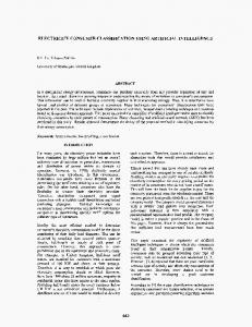
Fig. 1. Spatial maps and ternary pattern maps. Top row: the first derivatives of the Gaussian in the x and y directions, the input texture, and LOG filter. Middle row: the multi-resolution gradient maps and LOG response maps at scales σ1 = 1, σ2 = 2, σ3 = 4. Bottom row: the ternary pattern maps derived from the gradient maps and LOG response maps.

Algorithm 2 LOG-channel histogram representation Input: Normalized input image I Output: Histogram Hlog 1: Computation of LOG response maps L1 , L2 and L3 at scales σ1 , σ2 and σ3 ; 2: Neighboring sampling at a certain LOG response map Li , i ∈ {1, 2, 3}; 3: Computation of spectral maps LSk (k = 1, ..., K) via local 1-D DFT operator; 4: Ternary quantization of L1 , L2 and L3 ; 5: Binary quantization of LS1 , LS2 , ..., LSK ; 6: Joint space-frequency coding based on the quantized ternary and binary patterns; 7: Histogram representation Hlog .

B. Spectral map generation perform the multi-resolution spatial filtering via Gaussian first derivatives and Laplacian of Gaussian (LOG) filters. Specifically, the input image is first normalized to have zero mean and unit variance to reduce the effects of illumination changes [8], [13], [14]. Then, the rotation invariant gradient (magnitude) responses are obtained by √ G(x, y) = (I ⋆ Gx )2 + (I ⋆ Gy )2 (1) where I denotes the normalized image, Gx and Gy are the first derivatives of the Gaussian in the x and y directions, respectively, and ⋆ is the convolution operator. In our work, we compute Gaussian first derivatives at three scales: σi (i = 1, 2, 3). The resulting gradient (magnitude) response maps are denoted as G1 , G2 and G3 . Similarly, we compute the rotationally invariant LOG filtering responses at the same three scales and denote them as L1 , L2 and L3 . Fig. 1 (middle row) shows the extracted salient texture structures such as edges and bright/dark blobs, etc. Algorithm 1 Gradient-channel histogram representation Input: Normalized input image I Output: Histogram Hgrad 1: Multi-resolution spatial filtering via Gaussian first derivatives at scales σ1 , σ2 and σ3 ; 2: Computation of gradient maps G1 , G2 and G3 ; 3: Neighboring sampling at a certain gradient map Gi , i ∈ {1, 2, 3}; 4: Computation of spectral maps GSk (k = 1, ..., K) via local 1-D DFT operator; 5: Ternary quantization of G1 , G2 and G3 ; 6: Binary quantization of GS1 , GS2 , ..., GSK ; 7: Joint space-frequency coding based on the quantized ternary and binary patterns; 8: Histogram representation Hgrad .

To further consider longer-range pixel interactions and extract discriminative yet robust compact features, we apply the Fourier Transform (FT) to the spatial map to obtain pixel-wise frequency features. This is different from [10]–[12] where the local Fourier transform was performed in the original image space. Fig. 2 depicts the pipeline of spectral map generation. Given a spatial map Gi , let us consider the reference pixel (x, y) on Gi . First, we use the LBP-like [4] pixel sampling to obtain P neighbors Tp = [g1 , g2 , ..., gP ] on a circle of radius R centered at pixel (x, y). Next, we apply 1-D Discrete Fourier Transform (DFT) to Tp to extract local frequency features. Then, we keep the first K (K ≤ P/2 + 1) magnitude components in view of the symmetric property of Fourier coefficients. This step also gives the rotation invariance and preserves the main energy of the texture [11]. Finally, these magnitude components are L-2 normalized to be robust to illumination changes. The resulting feature vector is used as the spectral responses of pixel (x, y). In this work, we choose one gradient map Gi , i ∈ {1, 2, 3} to compute its K spectral maps GSk (k = 1, ..., K). Similarly, K LOG spectral maps LSk can be generated based on a certain LOG map Li , i ∈ {1, 2, 3}. C. Space-frequency co-occurrence histogram construction To explore the information of different feature domains, the spatial maps Gi , Li and spectral maps GSk , LSk are first quantized into three levels and two levels via global thresholding. Then, these quantized patterns are jointly encoded to construct a space-frequency co-occurrence histogram. •

Local ternary quantization (LTQ-I). For the gradient channel, the following operator is defined on Gi (i = 1, 2, 3):   2, Gi (x, y) > (1 + τ )mi 0, Gi (x, y) < (1 − τ )mi tqi (x, y) = (2)  1, otherwise where τ is a control parameter, and mi is a global

887

Fig. 2. Local frequency feature extraction and the binary quantization of spectral maps in the gradient channel. Two different reference pixels in the spatial map are highlighted in red and green to show their corresponding operators.

threshold defined by the mean of the spatial map: ∑ 1 mi = Gi (x, y) |Gi |

discriminative power of our coarse quantization. For the gradient channel, we perform the following coding: (3)

(x,y)∈Gi

•

where | · | denotes the cardinality. Fig. 1 (bottom row) shows the generated three ternary pattern maps at three corresponding scales. Local ternary quantization (LTQ-II). Since the LOG filers contain the sign information, we adopt the signed quantization for Li (i = 1, 2, 3)):   2, Li (x, y) > m+ i + tqi (x, y) = (4) 0, Li (x, y) < m− i  1, otherwise − where m+ i and mi are global thresholds which are defined by the means of positive and negative spatial responses, respectively: ∑ 1 (5) Li (x, y) m+ = i |L+ i | (x,y)∈L ,L (x,y)>0 i

m− i

i

∑ 1 = − Li (x, y) |Li | (x,y)∈L ,L (x,y) mk bqk (x, y) = (7) 0, otherwise

where the global threshold mk is determined by the mean of the spectral responses, which is similar to CLBP [8]: ∑ 1 mk = GSk (x, y) (8) |GSk | (x,y)∈GSk

•

Gcode (x, y) =

The similar operator is performed on the spectral maps LSk (k = 1, ..., K). The generated binary pattern maps in the gradient channel are shown in Fig. 2. Space-frequency co-occurrence histogram. The quantized binary and ternary patterns in the space-frequency domain are jointly encoded. It can also enhance the

K ∑

bqk (x, y)2k−1 + 2K

3 ∑

tqi (x, y)3i−1

i=1

k=1

(9) where tqi (x, y) and bqk (x, y) are defined on the spatial map Gi and the spectral map GSk , respectively. Then, we build a space-frequency co-occurrence histogram by ∑ Hgrad (l) = δ(Gcode (x, y) == l) (10) x,y

where l ∈ {0, 1, ..., 27 × 2K − 1}, and { 1, if z is true δ(z) = 0, otherwise

(11)

Similarly, we can build the co-occurrence histogram Hlog for the LOG channel (LTQ-II is utilized here). D. Texture feature representation The two-channel histograms are finally concatenated to form our texture representation H = [Hgrad Hlog ]. For simplicity, we hereinafter use the following naming convention. For example, if we use G3 with the sampling radius R = 2 to generate spectral maps in the gradient channel, and use L1 with R = 3 to generate spectral maps in the LOG channel, the resulting texture representation will be denoted as G3 L1 R23 . III. E XPERIMENTS We evaluate our method against the state-of-the-art LBPbased and learning-based approaches on the Outex database1 . We use two test suites: Outex TC 00010 (TC10) and Outex TC 00012 (TC12), which have the same 24 texture classes and 20 (128×128) samples per class captured under 9 rotation angles (0◦ , 5◦ ,10◦ , 15◦ , 30◦ , 45◦ , 60◦ , 75◦ and 90◦ ) and 3 different illuminants (“inca”, “horizon”and “t184”). For both test suites, the 480 (24×20) samples of illuminant “inca” and angle 0◦ are used for training. The TC10 is used for rotation test: the 3840 (24×20×8) samples under other 8 rotation angles are used for testing. The TC12 is used for rotation and illumination invariance test: all 4320 (24×20×9) samples of illuminant “t184” or “horizon” are used for testing.

888

1 http://www.outex.oulu.fi/

TABLE I C LASSIFICATION ACCURACY (%) ON THE O UTEX DATABASE

IV. C ONCLUSION In this paper, we have proposed to explore the joint statistical representation in the space-frequency domain with local quantized patterns for texture classification. The multiresolution spatial filters are adopted in two separate channels. In each channel, the locally invariant frequency features are extracted, which are further quantized into several levels via global threshoding. Then, the joint space-frequency coding is explored to capture a richer description. Finally, the twochannel features are combined to represent the texture. Experiments on the Outex texture database demonstrate that our method outperforms state-of-the-art approaches.

Method TC10 TC12-t184 TC12-horizon LBP (R=2, P =16) 89.40 82.27 75.21 LBP (R=3, P =24) 95.08 85.05 80.79 LTP (R=2, P =16) 96.95 90.16 86.94 LTP (R=3, P =24) 98.20 93.59 89.42 CLBP S/M/C (R=2, P =16) 98.72 93.54 93.91 CLBP S/M/C (R=3, P =24) 98.93 95.32 94.54 CLBC S/M/C (R=2, P =16) 98.54 93.26 94.07 CLBC S/M/C (R=3, P =24) 98.78 94.00 93.24 98.83 93.59 94.26 CLBC CLBP (R=2, P =16) CLBC CLBP (R=3, P =24) 98.96 95.37 94.72 Multi-scale CLBP (R=1, 2, 3) 99.17 95.23 95.58 Multi-scale CLBC (R=1, 2, 3) 99.04 94.10 95.14 DLBP+NGF [6] (R=2, P =16) 99.1 93.2 90.4 DLBP+NGF [6] (R=3, P =24) 98.2 91.6 87.4 DNS+LBP [7] (R=2, P =16) 98.90 93.22 92.13 DNS+LBP [7] (R=3, P =24) 99.27 94.40 92.85 VZ MR8 [13] 93.59 92.55 92.82 VZ Joint [14] 92.00 91.41 92.06 best from Liu [15] 99.7 98.7 98.1 LFD [11] 99.38 98.77 98.66 Proposed (G3 L1 R22 ) 100.00 99.77 99.93 Proposed (G3 L1 R33 ) 99.97 99.93 100.00

ACKNOWLEDGMENT This work was partially supported by NSFC (No. 61271289), National High Technology Research and Development Program of China (863 Program, No. 2012AA011503), The Ph.D. Programs Foundation of Ministry of Education of China (No. 20110185110002), and Academic Support Program for Excellent Ph.D. Students in UESTC (YBXSZC20131004).

TABLE II T HE BEST CLASSIFICATION ACCURACY (%) OF OUR METHOD ON THE O UTEX DATABASE BY SELECTING DIFFERENT CHANNELS

TC10 TC12-t184 TC12-horizon

Gradient

LOG

Gradient+LOG

99.43 98.59 99.58

99.69 99.49 99.51

100 99.93 100

R EFERENCES

Following [7]–[9], [15], the nearest neighborhood classifier with the Chi-square distance is used throughout our experiments. The results of LBP, LTP, CLBP, CLBC and their variants are from our own implementations, while the results of other methods are from the related literatures. For our method, we compute the spatial filtering at three scales: σ1 = 1, σ2 = 2, σ3 = 4, and we set τ = 0.4. For the compact representation, we set the number of spectral maps K = 5, resulting in 27 × 2K × 2 = 1728 dimensional features. Table I presents the comparison results. We can see that the proposed method consistently outperforms the state of the art for all three test settings, demonstrating its robustness to rotation and illumination changes. By exploring the joint statistics of local quantized patterns in the space-frequency domain, our method outperforms the space-based multi-scale CLBP and [15] and the frequency-based LFD [11]. Table II further reveals that the gradient and LOG channels can provide complementary information and combing them leads to the best performance. To our best knowledge, we are the first to report the perfect recognition rate of 100% on the Outex database. As opposed to the high-dimensional multiscale CLBP (2200), CLBC (1990) and [15] (2200), our representation has 1728-dimensional features thanks to our compact quantization patterns. In addition, unlike the textonbased VZ MR8 [13] and VZ Joint [14], our method is trainfree and needs no costly clustering.

[1] T. Song and H. Li, “Local polar dct features for image description,” IEEE Signal Process. Lett., vol. 20, no. 1, pp. 59–62, 2013. [2] B. S. Manjunath and W. Y. Ma, “Texture features for browsing and retrieval of image data,” IEEE Trans. Pattern Anal. Mach. Intell., vol. 18, no. 8, pp. 837–842, Aug. 1996. [3] T. Song and H. Li, “Wavelbp based hierarchical features for image classification,” Pattern Recogn. Lett., vol. 34, no. 12, pp. 1323–1328, 2013. [4] T. Ojala, M. Pietik¨ainen, and T. M¨aenp¨aa¨ , “Multiresolution gray-scale and rotation invariant texture classification with local binary patterns,” IEEE Trans. Pattern Anal. Mach. Intell., vol. 24, no. 7, pp. 971–987, Jul. 2002. [5] X. Tan and B. Triggs, “Enhanced local texture feature sets for face recognition under difficult lighting conditions,” IEEE Trans. Image Process., vol. 19, no. 6, pp. 1635–1650, Jun. 2010. [6] S. Liao, M. Law, and A. Chung, “Dominant local binary patterns for texture classification,” IEEE Trans. Image Process., vol. 18, no. 5, pp. 1107–1118, May. 2009. [7] F. Khellah, “Texture classification using dominant neighborhood structure,” IEEE Trans. Image Process., vol. 20, no. 11, pp. 3270–3279, Nov. 2011. [8] Z. Guo, L. Zhang, and D. Zhang, “A completed modeling of local binary pattern operator for texture classification,” IEEE Trans. Image Process., vol. 19, no. 6, pp. 1657–1663, Jun. 2010. [9] Y. Zhao, D.-S. Huang, and W. Jia, “Completed local binary count for rotation invariant texture classification,” IEEE Trans. Image Process., vol. 21, no. 10, pp. 4492–4497, Oct. 2012. [10] H. Arof and F. Deravi, “Circular neighbourhood and 1-d dft features for texture classification and segmentation,” IEE Proceedings on Vision, Image and Signal Processing, vol. 145, no. 3, pp. 167–172, Jun. 1998. [11] R. Maani, S. Kalra, and Y. Yang, “Rotation invariant local frequency descriptors for texture classification,” IEEE Trans. Image Process., vol. 22, no. 6, pp. 2409–2419, Jun. 2013. [12] F. Zhou, J. F. Feng, and Q. Y. Shi, “Texture feature based on local fourier transform,” in ICIP, 2001, pp. 610–613. [13] M. Varma and A. Zisserman, “A statistical approach to texture classification from single images,” Int. J. Comput. Vision, vol. 62, no. 1-2, pp. 61–81, Apr. 2005. [14] ——, “A statistical approach to material classification using image patch exemplars,” IEEE Trans. Pattern Anal. Mach. Intell., vol. 31, no. 11, pp. 2032–2047, Nov. 2009. [15] L. Liu, L. Zhao, Y. Long, G. Kuang, and P. Fieguth, “Extended local binary patterns for texture classification,” Image Vision Comput., vol. 30, no. 2, pp. 86–99, Feb. 2012.

889