The CLUSTER procedure hierarchically clusters the observations in a SAS data
set using one of ..... With METHOD=WARD, the NONORM option prevents the.
Chapter 23
The CLUSTER Procedure
Chapter Table of Contents OVERVIEW . . . . . . . . . . . . . . . . . . . . . . . . . . . . . . . . . . . 835 GETTING STARTED . . . . . . . . . . . . . . . . . . . . . . . . . . . . . . 837 SYNTAX . . . . . . . . . . . PROC CLUSTER Statement BY Statement . . . . . . . . COPY Statement . . . . . . FREQ Statement . . . . . . ID Statement . . . . . . . . RMSSTD Statement . . . . VAR Statement . . . . . . .
. . . . . . . .
. . . . . . . .
. . . . . . . .
. . . . . . . .
. . . . . . . .
. . . . . . . .
. . . . . . . .
. . . . . . . .
. . . . . . . .
. . . . . . . .
. . . . . . . .
. . . . . . . .
. . . . . . . .
. . . . . . . .
. . . . . . . .
. . . . . . . .
. . . . . . . .
. . . . . . . .
. . . . . . . .
. . . . . . . .
. . . . . . . .
. . . . . . . .
. . . . . . . .
. . . . . . . .
. . . . . . . .
. . . . . . . .
844 844 851 851 852 852 853 853
DETAILS . . . . . . . . . . . Clustering Methods . . . . . Miscellaneous Formulas . . Ultrametrics . . . . . . . . . Algorithms . . . . . . . . . Computational Resources . . Missing Values . . . . . . . Ties . . . . . . . . . . . . . Size, Shape, and Correlation Output Data Set . . . . . . . Displayed Output . . . . . . ODS Table Names . . . . .
. . . . . . . . . . . .
. . . . . . . . . . . .
. . . . . . . . . . . .
. . . . . . . . . . . .
. . . . . . . . . . . .
. . . . . . . . . . . .
. . . . . . . . . . . .
. . . . . . . . . . . .
. . . . . . . . . . . .
. . . . . . . . . . . .
. . . . . . . . . . . .
. . . . . . . . . . . .
. . . . . . . . . . . .
. . . . . . . . . . . .
. . . . . . . . . . . .
. . . . . . . . . . . .
. . . . . . . . . . . .
. . . . . . . . . . . .
. . . . . . . . . . . .
. . . . . . . . . . . .
. . . . . . . . . . . .
. . . . . . . . . . . .
. . . . . . . . . . . .
. . . . . . . . . . . .
. . . . . . . . . . . .
. . . . . . . . . . . .
854 854 861 863 863 864 865 865 866 867 870 872
EXAMPLES . . . . . . . . . . . . . . . . . . . . . Example 23.1 Cluster Analysis of Flying Mileages Cities . . . . . . . . . . . . . . . . Example 23.2 Crude Birth and Death Rates . . . . Example 23.3 Cluster Analysis of Fisher Iris Data . Example 23.4 Evaluating the Effects of Ties . . . . Example 23.5 Computing a Distance Matrix . . . . Example 23.6 Size, Shape, and Correlation . . . .
. . . . . . . . . . . . . between Ten American . . . . . . . . . . . . . . . . . . . . . . . . . . . . . . . . . . . . . . . . . . . . . . . . . . . . . . . . . . . . . . . . . . . . . . . . . . . . . .
. 873 . . . . . .
873 880 889 902 916 921
REFERENCES . . . . . . . . . . . . . . . . . . . . . . . . . . . . . . . . . . 941
834 �
Chapter 23. The CLUSTER Procedure
SAS OnlineDoc: Version 8
Chapter 23
The CLUSTER Procedure Overview The CLUSTER procedure hierarchically clusters the observations in a SAS data set using one of eleven methods. The CLUSTER procedure finds hierarchical clusters of the observations in a SAS data set. The data can be coordinates or distances. If the data are coordinates, PROC CLUSTER computes (possibly squared) Euclidean distances. If you want to perform a cluster analysis on non-Euclidean distance data, it is possible to do so by using a TYPE=DISTANCE data set as input. The %DISTANCE macro in the SAS/STAT sample library can compute many kinds of distance matrices. One situation where analyzing non-Euclidean distance data can be useful is when you have categorical data, where the distance data are calculated using an association measure. For more information, see Example 23.5 on page 916. The clustering methods available are average linkage, the centroid method, complete linkage, density linkage (including Wong’s hybrid and k th-nearest-neighbor methods), maximum likelihood for mixtures of spherical multivariate normal distributions with equal variances but possibly unequal mixing proportions, the flexible-beta method, McQuitty’s similarity analysis, the median method, single linkage, two-stage density linkage, and Ward’s minimum-variance method. All methods are based on the usual agglomerative hierarchical clustering procedure. Each observation begins in a cluster by itself. The two closest clusters are merged to form a new cluster that replaces the two old clusters. Merging of the two closest clusters is repeated until only one cluster is left. The various clustering methods differ in how the distance between two clusters is computed. Each method is described in the section “Clustering Methods” on page 854. The CLUSTER procedure is not practical for very large data sets because, with most methods, the CPU time varies as the square or cube of the number of observations. The FASTCLUS procedure requires time proportional to the number of observations and can, therefore, be used with much larger data sets than PROC CLUSTER. If you want to cluster a very large data set hierarchically, you can use PROC FASTCLUS for a preliminary cluster analysis producing a large number of clusters and then use PROC CLUSTER to cluster the preliminary clusters hierarchically. This method is used to find clusters for the Fisher Iris data in Example 23.3, later in this chapter. PROC CLUSTER displays a history of the clustering process, giving statistics useful for estimating the number of clusters in the population from which the data are sampled. PROC CLUSTER also creates an output data set that can be used by the TREE procedure to draw a tree diagram of the cluster hierarchy or to output the cluster membership at any desired level. For example, to obtain the six-cluster so-
836 �
Chapter 23. The CLUSTER Procedure lution, you could first use PROC CLUSTER with the OUTTREE= option then use this output data set as the input data set to the TREE procedure. With PROC TREE, specify NCLUSTERS=6 and the OUT= options to obtain the six-cluster solution and draw a tree diagram. For an example, see Example 66.1 in Chapter 66, “The TREE Procedure.” Before you perform a cluster analysis on coordinate data, it is necessary to consider scaling or transforming the variables since variables with large variances tend to have more effect on the resulting clusters than those with small variances. The ACECLUS procedure is useful for performing linear transformations of the variables. You can also use the PRINCOMP procedure with the STD option, although in some cases it tends to obscure clusters or magnify the effect of error in the data when all components are retained. The STD option in the CLUSTER procedure standardizes the variables to mean 0 and standard deviation 1. Standardization is not always appropriate. See Milligan and Cooper (1987) for a Monte Carlo study on various methods of variable standardization. You should remove outliers before using PROC PRINCOMP or before using PROC CLUSTER with the STD option unless you specify the TRIM= option. Nonlinear transformations of the variables may change the number of population clusters and should, therefore, be approached with caution. For most applications, the variables should be transformed so that equal differences are of equal practical importance. An interval scale of measurement is required if raw data are used as input. Ordinal or ranked data are generally not appropriate. Agglomerative hierarchical clustering is discussed in all standard references on cluster analysis, for example, Anderberg (1973), Sneath and Sokal (1973), Hartigan (1975), Everitt (1980), and Spath (1980). An especially good introduction is given by Massart and Kaufman (1983). Anyone considering doing a hierarchical cluster analysis should study the Monte Carlo results of Milligan (1980), Milligan and Cooper (1985), and Cooper and Milligan (1988). Other essential, though more advanced, references on hierarchical clustering include Hartigan (1977, pp. 60–68; 1981), Wong (1982), Wong and Schaack (1982), and Wong and Lane (1983). Refer to Blashfield and Aldenderfer (1978) for a discussion of the confusing terminology in hierarchical cluster analysis.
SAS OnlineDoc: Version 8
Getting Started
�
837
Getting Started The following example demonstrates how you can use the CLUSTER procedure to compute hierarchical clusters of observations in a SAS data set. Suppose you want to determine whether national figures for birth rates, death rates, and infant death rates can be used to determine certain types or categories of countries. You want to perform a cluster analysis to determine whether the observations can be formed into groups suggested by the data. Previous studies indicate that the clusters computed from this type of data can be elongated and elliptical. Thus, you need to perform some linear transformation on the raw data before the cluster analysis. The following data� from Rouncefield (1995) are birth rates, death rates, and infant death rates for 97 countries. The DATA step creates the SAS data set Poverty: data Poverty; input Birth Death InfantDeath Country $20. @@; datalines; 24.7 5.7 30.8 Albania 12.5 11.9 14.4 Bulgaria 13.4 11.7 11.3 Czechoslovakia 12 12.4 7.6 Former_E._Germany 11.6 13.4 14.8 Hungary 14.3 10.2 16 Poland 13.6 10.7 26.9 Romania 14 9 20.2 Yugoslavia 17.7 10 23 USSR 15.2 9.5 13.1 Byelorussia_SSR 13.4 11.6 13 Ukrainian_SSR 20.7 8.4 25.7 Argentina 46.6 18 111 Bolivia 28.6 7.9 63 Brazil 23.4 5.8 17.1 Chile 27.4 6.1 40 Columbia 32.9 7.4 63 Ecuador 28.3 7.3 56 Guyana 34.8 6.6 42 Paraguay 32.9 8.3 109.9 Peru 18 9.6 21.9 Uruguay 27.5 4.4 23.3 Venezuela 29 23.2 43 Mexico 12 10.6 7.9 Belgium 13.2 10.1 5.8 Finland 12.4 11.9 7.5 Denmark 13.6 9.4 7.4 France 11.4 11.2 7.4 Germany 10.1 9.2 11 Greece 15.1 9.1 7.5 Ireland 9.7 9.1 8.8 Italy 13.2 8.6 7.1 Netherlands 14.3 10.7 7.8 Norway 11.9 9.5 13.1 Portugal 10.7 8.2 8.1 Spain 14.5 11.1 5.6 Sweden 12.5 9.5 7.1 Switzerland 13.6 11.5 8.4 U.K. 14.9 7.4 8 Austria 9.9 6.7 4.5 Japan 14.5 7.3 7.2 Canada 16.7 8.1 9.1 U.S.A. 40.4 18.7 181.6 Afghanistan 28.4 3.8 16 Bahrain 42.5 11.5 108.1 Iran 42.6 7.8 69 Iraq 22.3 6.3 9.7 Israel 38.9 6.4 44 Jordan 26.8 2.2 15.6 Kuwait 31.7 8.7 48 Lebanon 45.6 7.8 40 Oman 42.1 7.6 71 Saudi_Arabia 29.2 8.4 76 Turkey 22.8 3.8 26 United_Arab_Emirates 42.2 15.5 119 Bangladesh 41.4 16.6 130 Cambodia 21.2 6.7 32 China 11.7 4.9 6.1 Hong_Kong 30.5 10.2 91 India 28.6 9.4 75 Indonesia 23.5 18.1 25 Korea 31.6 5.6 24 Malaysia 36.1 8.8 68 Mongolia 39.6 14.8 128 Nepal � These data have been compiled from the United Nations Demographic Yearbook 1990 (United
Nations publications, Sales No. E/F.91.XII.1, copyright 1991, United Nations, New York) and are reproduced with the permission of the United Nations.
SAS OnlineDoc: Version 8
838 �
Chapter 23. The CLUSTER Procedure 30.3 17.8 22.3 35.5 48.5 38.8 39.4 44.4 44 35.5 44 48.2 32.1 46.8 52.2 45.6 41.7 ;
8.1 107.7 Pakistan 5.2 7.5 Singapore 7.7 28 Thailand 8.3 74 Algeria 11.6 67 Botswana 9.5 49.4 Egypt 16.8 103 Gabon 13.1 90 Ghana 9.4 82 Libya 9.8 82 Morocco 12.1 135 Namibia 23.4 154 Sierra_Leone 9.9 72 South_Africa 12.5 118 Swaziland 15.6 103 Uganda 14.2 83 Zaire 10.3 66 Zimbabwe
33.2 21.3 31.8 47.2 46.1 48.6 47.4 47 48.3 45 48.5 50.1 44.6 31.1 50.5 51.1
7.7 6.2 9.5 20.2 14.6 20.7 21.4 11.3 25 18.5 15.6 20.2 15.8 7.3 14 13.7
45 19.4 64 137 73 137 143 72 130 141 105 132 108 52 106 80
Philippines Sri_Lanka Vietnam Angola Congo Ethiopia Gambia Kenya Malawi Mozambique Nigeria Somalia Sudan Tunisia Tanzania Zambia
The data set Poverty contains the character variable Country and the numeric variables Birth, Death, and InfantDeath, which represent the birth rate per thousand, death rate per thousand, and infant death rate per thousand. The $20. in the INPUT statement specifies that the variable Country is a character variable with a length of 20. The double trailing at sign (@@) in the INPUT statement holds the input line for further iterations of the DATA step, specifying that observations are input from each line until all values are read. Because the variables in the data set do not have equal variance, you must perform some form of scaling or transformation. One method is to standardize the variables to mean zero and variance one. However, when you suspect that the data contain elliptical clusters, you can use the ACECLUS procedure to transform the data such that the resulting within-cluster covariance matrix is spherical. The procedure obtains approximate estimates of the pooled within-cluster covariance matrix and then computes canonical variables to be used in subsequent analyses. The following statements perform the ACECLUS transformation using the SAS data set Poverty. The OUT= option creates an output SAS data set called Ace to contain the canonical variable scores. proc aceclus data=Poverty out=Ace p=.03 noprint; var Birth Death InfantDeath; run;
The P= option specifies that approximately three percent of the pairs are included in the estimation of the within-cluster covariance matrix. The NOPRINT option suppresses the display of the output. The VAR statement specifies that the variables Birth, Death, and InfantDeath are used in computing the canonical variables. The following statements invoke the CLUSTER procedure, using the SAS data set ACE created in the previous PROC ACECLUS run.
SAS OnlineDoc: Version 8
Getting Started
�
839
proc cluster data=Ace outtree=Tree method=ward ccc pseudo print=15; var can1 can2 can3 ; id Country; run;
The OUTTREE= option creates an output SAS data set called Tree that can be used by the TREE procedure to draw a tree diagram. Ward’s minimum-variance clustering method is specified by the METHOD= option. The CCC option displays the cubic clustering criterion, and the PSEUDO option displays pseudo F and t2 statistics. Only the last 15 generations of the cluster history are displayed, as defined by the PRINT= option. The VAR statement specifies that the canonical variables computed in the ACECLUS procedure are used in the cluster analysis. The ID statement specifies that the variable Country should be added to the Tree output data set. The results of this analysis are displayed in the following figures. PROC CLUSTER first displays the table of eigenvalues of the covariance matrix for the three canonical variables (Figure 23.1). The first two columns list each eigenvalue and the difference between the eigenvalue and its successor. The last two columns display the individual and cumulative proportion of variation associated with each eigenvalue. The CLUSTER Procedure Ward’s Minimum Variance Cluster Analysis Eigenvalues of the Covariance Matrix
1 2 3
Eigenvalue
Difference
Proportion
Cumulative
64.5500051 9.8186828 5.4148519
54.7313223 4.4038309
0.8091 0.1231 0.0679
0.8091 0.9321 1.0000
Root-Mean-Square Total-Sample Standard Deviation = 5.156987 Root-Mean-Square Distance Between Observations = 12.63199
Figure 23.1.
Table of Eigenvalues of the Covariance Matrix
As displayed in the last column, the first two canonical variables account for about 93% of the total variation. Figure 23.1 also displays the root mean square of the total sample standard deviation and the root mean square distance between observations. Figure 23.2 displays the last 15 generations of the cluster history. First listed are the number of clusters and the names of the clusters joined. The observations are identified either by the ID value or by CLn, where n is the number of the cluster. Next, PROC CLUSTER displays the number of observations in the new cluster and the semipartial R2 . The latter value represents the decrease in the proportion of variance accounted for by joining the two clusters.
SAS OnlineDoc: Version 8
840 �
Chapter 23. The CLUSTER Procedure The CLUSTER Procedure Ward’s Minimum Variance Cluster Analysis Root-Mean-Square Total-Sample Standard Deviation = 5.156987 Root-Mean-Square Distance Between Observations = 12.63199
Cluster History
NCL 15 14 13 12 11 10 9 8 7 6 5 4 3 2 1
--------------Clusters Joined--------------Oman CL31 CL41 CL19 CL39 CL76 CL23 CL10 CL9 CL8 CL14 CL16 CL12 CL3 CL5
CL37 CL22 CL17 CL21 CL15 CL27 CL11 Afghanistan CL25 CL20 CL13 CL7 CL6 CL4 CL2
Figure 23.2.
FREQ
SPRSQ
RSQ
ERSQ
CCC
PSF
PST2
5 13 32 10 9 6 15 7 17 14 45 28 24 52 97
0.0039 0.0040 0.0041 0.0045 0.0052 0.0075 0.0130 0.0134 0.0217 0.0239 0.0307 0.0323 0.0323 0.1782 0.5866
.957 .953 .949 .945 .940 .932 .919 .906 .884 .860 .829 .797 .765 .587 .000
.933 .928 .922 .916 .909 .900 .890 .879 .864 .846 .822 .788 .732 .613 .000
6.03 5.81 5.70 5.65 5.60 5.25 4.20 3.55 2.26 1.42 0.65 0.57 1.84 -.82 0.00
132 131 131 132 134 133 125 122 114 112 112 122 153 135 .
12.1 9.7 13.1 6.4 6.3 18.1 12.4 7.3 11.6 10.5 59.2 14.8 11.6 48.9 135
Cluster Generation History and R-Square Values
Next listed is the squared multiple correlation, R2 , which is the proportion of variance accounted for by the clusters. Figure 23.2 shows that, when the data are grouped into three clusters, the proportion of variance accounted for by the clusters (R2 ) is about 77%. The approximate expected value of R2 is given in the column labeled “ERSQ.” The next three columns display the values of the cubic clustering criterion (CCC), pseudo F (PSF), and t2 (PST2) statistics. These statistics are useful in determining the number of clusters in the data. Values of the cubic clustering criterion greater than 2 or 3 indicate good clusters; values between 0 and 2 indicate potential clusters, but they should be considered with caution; large negative values can indicate outliers. In Figure 23.2, there is a local peak of the CCC when the number of clusters is 3. The CCC drops at 4 clusters and then steadily increases, levelling off at 11 clusters. Another method of judging the number of clusters in a data set is to look at the pseudo F statistic (PSF). Relatively large values indicate a stopping point. Reading down the PSF column, you can see that this method indicates a possible stopping point at 11 clusters and another at 3 clusters. A general rule for interpreting the values of the pseudo t2 statistic is to move down the column until you find the first value markedly larger than the previous value and move back up the column by one cluster. Moving down the PST2 column, you can see possible clustering levels at 11 clusters, 6 clusters, 3 clusters, and 2 clusters. The final column in Figure 23.2 lists ties for minimum distance; a blank value indicates the absence of a tie. These statistics indicate that the data can be clustered into 11 clusters or 3 clusters. The following statements examine the results of clustering the data into 3 clusters.
SAS OnlineDoc: Version 8
T i e
Getting Started
�
841
A graphical view of the clustering process can often be helpful in interpreting the clusters. The following statements use the TREE procedure to produce a tree diagram of the clusters: goptions vsize=8in htext=1pct htitle=2.5pct; axis1 order=(0 to 1 by 0.2); proc tree data=Tree out=New nclusters=3 graphics haxis=axis1 horizontal; height _rsq_; copy can1 can2 ; id country; run;
The AXIS1 statement defines axis parameters that are used in the TREE procedure. The ORDER= option specifies the data values in the order in which they should appear on the axis. The preceding statements use the SAS data set Tree as input. The OUT= option creates an output SAS data set named New to contain information on cluster membership. The NCLUSTERS= option specifies the number of clusters desired in the data set New. The GRAPHICS option directs the procedure to use high resolution graphics. The HAXIS= option specifies AXIS1 to customize the appearance of the horizontal axis. Use this option only when the GRAPHICS option is in effect. The HORIZONTAL option orients the tree diagram horizontally. The HEIGHT statement specifies the variable – RSQ– (R2 ) as the height variable. The COPY statement copies the canonical variables can1 and can2 (computed in the ACECLUS procedure) into the output SAS data set New. Thus, the SAS output data set New contains information for three clusters and the first two of the original canonical variables. Figure 23.3 displays the tree diagram. The figure provides a graphical view of the information in Figure 23.2. As the number of branches grows to the left from the root, the R2 approaches 1; the first three clusters (branches of the tree) account for over half of the variation (about 77%, from Figure 23.2). In other words, only three clusters are necessary to explain over three-fourths of the variation.
SAS OnlineDoc: Version 8
842 �
Chapter 23. The CLUSTER Procedure
Figure 23.3.
SAS OnlineDoc: Version 8
Tree Diagram of Clusters versus R-Square Values
Getting Started
�
843
The following statements invoke the GPLOT procedure on the SAS data set New. legend1 frame cframe=ligr cborder=black position=center value=(justify=center); axis1 label=(angle=90 rotate=0) minor=none order=(-10 to 20 by 5); axis2 minor=none order=(-10 to 20 by 5); proc gplot data=New ; plot can2*can1=cluster/frame cframe=ligr legend=legend1 vaxis=axis1 haxis=axis2; run;
The PLOT statement requests a plot of the two canonical variables, using the value of the variable cluster as the identification variable. Figure 23.4 displays the separation of the clusters when three clusters are calculated. The plotting symbol is the cluster number.
Figure 23.4.
Plot of Canonical Variables and Cluster for Three Clusters
The statistics in Figure 23.2, the tree diagram in Figure 23.3, and the plot of the canonical variables assist in the determination of clusters in the data. There seems to be reasonable separation in the clusters. However, you must use this information, along with experience and knowledge of the field, to help in deciding the correct number of clusters.
SAS OnlineDoc: Version 8
844 �
Chapter 23. The CLUSTER Procedure
Syntax The following statements are available in the CLUSTER procedure.
PROC CLUSTER METHOD = name < options > ; BY variables ; COPY variables ; FREQ variable ; ID variable ; RMSSTD variable ; VAR variables ; Only the PROC CLUSTER statement is required, except that the FREQ statement is required when the RMSSTD statement is used; otherwise the FREQ statement is optional. Usually only the VAR statement and possibly the ID and COPY statements are needed in addition to the PROC CLUSTER statement. The rest of this section provides detailed syntax information for each of the preceding statements, beginning with the PROC CLUSTER statement. The remaining statements are covered in alphabetical order.
PROC CLUSTER Statement PROC CLUSTER METHOD=name < options > ; The PROC CLUSTER statement starts the CLUSTER procedure, identifies a clustering method, and optionally identifies details for clustering methods, data sets, data processing, and displayed output. The METHOD= specification determines the clustering method used by the procedure. Any one of the following 11 methods can be specified for name: AVERAGE | AVE
requests average linkage (group average, unweighted pairgroup method using arithmetic averages, UPGMA). Distance data are squared unless you specify the NOSQUARE option.
CENTROID | CEN
requests the centroid method (unweighted pair-group method using centroids, UPGMC, centroid sorting, weighted-group method). Distance data are squared unless you specify the NOSQUARE option.
COMPLETE | COM
requests complete linkage (furthest neighbor, maximum method, diameter method, rank order typal analysis). To reduce distortion of clusters by outliers, the TRIM= option is recommended.
DENSITY | DEN
requests density linkage, which is a class of clustering methods using nonparametric probability density estima-
SAS OnlineDoc: Version 8
PROC CLUSTER Statement
�
845
tion. You must also specify one of the K=, R=, or HYBRID options to indicate the type of density estimation to be used. See also the MODE= and DIM= options in this section. EML
requests maximum-likelihood hierarchical clustering for mixtures of spherical multivariate normal distributions with equal variances but possibly unequal mixing proportions. Use METHOD=EML only with coordinate data. See the PENALTY= option on page 849. The NONORM option does not affect the reported likelihood values but does affect other unrelated criteria. The EML method is much slower than the other methods in the CLUSTER procedure.
FLEXIBLE | FLE
requests the Lance-Williams flexible-beta method. See the BETA= option in this section.
MCQUITTY | MCQ
requests McQuitty’s similarity analysis, which is weighted average linkage, weighted pair-group method using arithmetic averages (WPGMA).
MEDIAN | MED
requests Gower’s median method, which is weighted pairgroup method using centroids (WPGMC). Distance data are squared unless you specify the NOSQUARE option.
SINGLE | SIN
requests single linkage (nearest neighbor, minimum method, connectedness method, elementary linkage analysis, or dendritic method). To reduce chaining, you can use the TRIM= option with METHOD=SINGLE.
TWOSTAGE | TWO
requests two-stage density linkage. You must also specify the K=, R=, or HYBRID option to indicate the type of density estimation to be used. See also the MODE= and DIM= options in this section.
WARD | WAR
requests Ward’s minimum-variance method (error sum of squares, trace W). Distance data are squared unless you specify the NOSQUARE option. To reduce distortion by outliers, the TRIM= option is recommended. See the NONORM option.
The following table summarizes the options in the PROC CLUSTER statement.
SAS OnlineDoc: Version 8
846 �
Chapter 23. The CLUSTER Procedure Tasks Specify input and output data sets specify input data set create output data set
Options DATA= OUTTREE=
Specify clustering methods specify clustering method beta for flexible beta method minimum number of members for modal clusters penalty coefficient for maximum-likelihood Wong’s hybrid clustering method
METHOD= BETA= MODE= PENALTY= HYBRID
Control data processing prior to clustering suppress computation of eigenvalues suppress normalizing of distances suppress squaring of distances standardize variables omit points with low probability densities
NOEIGEN NONORM NOSQUARE STANDARD TRIM=
Control density estimation dimensionality for estimates number of neighbors for k th-nearest-neighbor radius of sphere of support for uniform-kernel
DIM= K= R=
Suppress checking for ties
NOTIE
Control display of the cluster history display cubic clustering criterion suppress display of ID values specify number of generations to display display pseudo F and t2 statistics display root-mean-square standard deviation display R2 and semipartial R2
CCC NOID PRINT= PSEUDO RMSSTD RSQUARE
Control other aspects of output suppress display of all output display simple summary statistics
NOPRINT SIMPLE
The following list provides details on these options. BETA=n
specifies the beta parameter for METHOD=FLEXIBLE. The value of n should be less than 1, usually between 0 and ,1. By default, BETA=,0:25. Milligan (1987) suggests a somewhat smaller value, perhaps ,0:5, for data with many outliers.
CCC
displays the cubic clustering criterion and approximate expected R2 under the uniform null hypothesis (Sarle 1983). The statistics associated with the RSQUARE option, R2 and semipartial R2 , are also displayed. The CCC option applies only to coordinate data. The CCC option is not appropriate with METHOD=SINGLE because of the method’s tendency to chop off tails of distributions.
SAS OnlineDoc: Version 8
PROC CLUSTER Statement
�
847
DATA=SAS-data-set
names the input data set containing observations to be clustered. By default, the procedure uses the most recently created SAS data set. If the data set is TYPE=DISTANCE, the data are interpreted as a distance matrix; the number of variables must equal the number of observations in the data set or in each BY group. The distances are assumed to be Euclidean, but the procedure accepts other types of distances or dissimilarities. If the data set is not TYPE=DISTANCE, the data are interpreted as coordinates in a Euclidean space, and Euclidean distances are computed. For more on TYPE=DISTANCE data sets, see Appendix A, “Special SAS Data Sets.” You cannot use a TYPE=CORR data set as input to PROC CLUSTER, since the procedure uses dissimilarity measures. Instead, you can use a DATA step or the IML procedure to extract the correlation matrix from a TYPE=CORR data set and transform the values to dissimilarities such as 1,r or 1,r 2 , where r is the correlation. All methods produce the same results when used with coordinate data as when used with Euclidean distances computed from the coordinates. However, the DIM= option must be used with distance data if you specify METHOD=TWOSTAGE or METHOD=DENSITY or if you specify the TRIM= option. Certain methods that are most naturally defined in terms of coordinates require squared Euclidean distances to be used in the combinatorial distance formulas (Lance and Williams 1967). For this reason, distance data are automatically squared when used with METHOD=AVERAGE, METHOD=CENTROID, METHOD=MEDIAN, or METHOD=WARD. If you want the combinatorial formulas to be applied to the (unsquared) distances with these methods, use the NOSQUARE option. DIM=n
specifies the dimensionality used when computing density estimates with the TRIM= option, METHOD=DENSITY, or METHOD=TWOSTAGE. The values of n must be greater than or equal to 1. The default is the number of variables if the data are coordinates; the default is 1 if the data are distances. HYBRID
requests Wong’s (1982) hybrid clustering method in which density estimates are computed from a preliminary cluster analysis using the k -means method. The DATA= data set must contain means, frequencies, and root-mean-square standard deviations of the preliminary clusters (see the FREQ and RMSSTD statements). To use HYBRID, you must use either a FREQ statement or a DATA= data set that contains a – FREQ– variable, and you must also use either an RMSSTD statement or a DATA= data set that contains a – RMSSTD– variable. The MEAN= data set produced by the FASTCLUS procedure is suitable for input to the CLUSTER procedure for hybrid clustering. Since this data set contains – FREQ– and – RMSSTD– variables, you can use it as input and then omit the FREQ and RMSSTD statements. You must specify either METHOD=DENSITY or METHOD=TWOSTAGE with the HYBRID option. You cannot use this option in combination with the TRIM=, K=, or R= option.
SAS OnlineDoc: Version 8
848 �
Chapter 23. The CLUSTER Procedure
K=n
specifies the number of neighbors to use for k th-nearest-neighbor density estimation (Silverman 1986, pp. 19–21 and 96–99). The number of neighbors (n) must be at least two but less than the number of observations. See the MODE= option, which follows. If you request an analysis that requires density estimation (the TRIM= option, METHOD=DENSITY, or METHOD=TWOSTAGE), you must specify one of the K=, HYBRID, or R= options.
MODE=n
specifies that, when two clusters are joined, each must have at least n members for either cluster to be designated a modal cluster. If you specify MODE=1, each cluster must also have a maximum density greater than the fusion density for either cluster to be designated a modal cluster. Use the MODE= option only with METHOD=DENSITY or METHOD=TWOSTAGE. With METHOD=TWOSTAGE, the MODE= option affects the number of modal clusters formed. With METHOD=DENSITY, the MODE= option does not affect the clustering process but does determine the number of modal clusters reported on the output and identified by the – MODE– variable in the output data set. If you specify the K= option, the default value of MODE= is the same as the value of K= because the use of k th-nearest-neighbor density estimation limits the resolution that can be obtained for clusters with fewer than k members. If you do not specify the K= option, the default is MODE=2. If you specify MODE=0, the default value is used instead of 0. If you specify a FREQ statement or if a – FREQ– variable appears in the input data set, the MODE= value is compared with the number of actual observations in the clusters being joined, not with the sum of the frequencies in the clusters.
NOEIGEN
suppresses computation of eigenvalues for the cubic clustering criterion. Specifying the NOEIGEN option saves time if the number of variables is large, but it should be used only if the variables are nearly uncorrelated or if you are not interested in the cubic clustering criterion. If you specify the NOEIGEN option and the variables are highly correlated, the cubic clustering criterion may be very liberal. The NOEIGEN option applies only to coordinate data. NOID
suppresses the display of ID values for the clusters joined at each generation of the cluster history. NONORM
prevents the distances from being normalized to unit mean or unit root mean square with most methods. With METHOD=WARD, the NONORM option prevents the between-cluster sum of squares from being normalized by the total sum of squares to yield a squared semipartial correlation. The NONORM option does not affect the reported likelihood values with METHOD=EML, but it does affect other unrelated criteria, such as the – DIST– variable. SAS OnlineDoc: Version 8
PROC CLUSTER Statement
�
849
NOPRINT
suppresses the display of all output. Note that this option temporarily disables the Output Delivery System (ODS). For more information, see Chapter 15, “Using the Output Delivery System.” NOSQUARE
prevents input distances from being squared with METHOD=AVERAGE, METHOD=CENTROID, METHOD=MEDIAN, or METHOD=WARD. If you specify the NOSQUARE option with distance data, the data are assumed to be squared Euclidean distances for computing R-squared and related statistics defined in a Euclidean coordinate system. If you specify the NOSQUARE option with coordinate data with METHOD=CENTROID, METHOD=MEDIAN, or METHOD=WARD, then the combinatorial formula is applied to unsquared Euclidean distances. The resulting cluster distances do not have their usual Euclidean interpretation and are, therefore, labeled “False” in the output. NOTIE
prevents PROC CLUSTER from checking for ties for minimum distance between clusters at each generation of the cluster history. If your data are measured with such sufficient precision that ties are unlikely, then you can specify the NOTIE option to reduce slightly the time and space required by the procedure. See the section “Ties” on page 865. OUTTREE=SAS-data-set
creates an output data set that can be used by the TREE procedure to draw a tree diagram. You must give the data set a two-level name to save it. Refer to SAS Language Reference: Concepts for a discussion of permanent data sets. If you omit the OUTTREE= option, the data set is named using the DATAn convention and is not permanently saved. If you do not want to create an output data set, use OUTTREE=– NULL– . PENALTY=p
specifies the penalty coefficient used with METHOD=EML. See the section “Clustering Methods” on page 854. Values for p must be greater than zero. By default, PENALTY=2. PRINT=n | P=n
specifies the number of generations of the cluster history to display. The P= option displays the latest n generations; for example, P=5 displays the cluster history from 1 cluster through 5 clusters. The value of P= must be a nonnegative integer. The default is to display all generations. Specify PRINT=0 to suppress the cluster history. PSEUDO
displays pseudo F and t2 statistics. This option is effective only when the data are coordinates or when METHOD=AVERAGE, METHOD=CENTROID, or METHOD=WARD. See the section “Miscellaneous Formulas” on page 861. The PSEUDO option is not appropriate with METHOD=SINGLE because of the method’s tendency to chop off tails of distributions.
SAS OnlineDoc: Version 8
850 �
Chapter 23. The CLUSTER Procedure
R=n
specifies the radius of the sphere of support for uniform-kernel density estimation (Silverman 1986, pp. 11–13 and 75–94). The value of R= must be greater than zero. If you request an analysis that requires density estimation (the TRIM= option, METHOD=DENSITY, or METHOD=TWOSTAGE), you must specify one of the K=, HYBRID, or R= options. RMSSTD
displays the root-mean-square standard deviation of each cluster. This option is effective only when the data are coordinates or when METHOD=AVERAGE, METHOD=CENTROID, or METHOD=WARD. See the section “Miscellaneous Formulas” on page 861. RSQUARE | RSQ
displays the R2 and semipartial R2 . This option is effective only when the data are coordinates or when METHOD=AVERAGE or METHOD=CENTROID. The R2 and semipartial R2 statistics are always displayed with METHOD=WARD. See the section “Miscellaneous Formulas” on page 861.
SIMPLE | S
displays means, standard deviations, skewness, kurtosis, and a coefficient of bimodality. The SIMPLE option applies only to coordinate data. See the section “Miscellaneous Formulas” on page 861. STANDARD | STD
standardizes the variables to mean 0 and standard deviation 1. The STANDARD option applies only to coordinate data. TRIM=p
omits points with low estimated probability densities from the analysis. Valid values for the TRIM= option are 0 � p < 100. If p < 1, then p is the proportion of observations omitted. If p � 1, then p is interpreted as a percentage. A specification of TRIM=10, which trims 10 percent of the points, is a reasonable value for many data sets. Densities are estimated by the k th-nearest-neighbor or uniform-kernel methods. Trimmed points are indicated by a negative value of the – FREQ– variable in the OUTTREE= data set. You must use either the K= or R= option when you use TRIM=. You cannot use the HYBRID option in combination with TRIM=, so you may want to use the DIM= option instead. If you specify the STANDARD option in combination with TRIM=, the variables are standardized both before and after trimming. The TRIM= option is useful for removing outliers and reducing chaining. Trimming is highly recommended with METHOD=WARD or METHOD=COMPLETE because clusters from these methods can be severely distorted by outliers. Trimming is also valuable with METHOD=SINGLE since single linkage is the method most susceptible to chaining. Most other methods also benefit from trimming. However, trimming is unnecessary with METHOD=TWOSTAGE or METHOD=DENSITY when k th-nearest-neighbor density estimation is used.
SAS OnlineDoc: Version 8
COPY Statement
�
851
Use of the TRIM= option may spuriously inflate the cubic clustering criterion and the pseudo F and t2 statistics. Trimming only outliers improves the accuracy of the statistics, but trimming saddle regions between clusters yields excessively large values.
BY Statement BY variables ; You can specify a BY statement with PROC CLUSTER to obtain separate analyses on observations in groups defined by the BY variables. When a BY statement appears, the procedure expects the input data set to be sorted in order of the BY variables. If your input data set is not sorted in ascending order, use one of the following alternatives:
� �
�
Sort the data using the SORT procedure with a similar BY statement. Specify the BY statement option NOTSORTED or DESCENDING in the BY statement for the CLUSTER procedure. The NOTSORTED option does not mean that the data are unsorted but rather that the data are arranged in groups (according to values of the BY variables) and that these groups are not necessarily in alphabetical or increasing numeric order. Create an index on the BY variables using the DATASETS procedure.
For more information on the BY statement, refer to the discussion in SAS Language Reference: Concepts. For more information on the DATASETS procedure, refer to the discussion in the SAS Procedures Guide.
COPY Statement COPY variables ; The variables in the COPY statement are copied from the input data set to the OUTTREE= data set. Observations in the OUTTREE= data set that represent clusters of more than one observation from the input data set have missing values for the COPY variables.
SAS OnlineDoc: Version 8
852 �
Chapter 23. The CLUSTER Procedure
FREQ Statement FREQ variable ; If one variable in the input data set represents the frequency of occurrence for other values in the observation, specify the variable’s name in a FREQ statement. PROC CLUSTER then treats the data set as if each observation appeared n times, where n is the value of the FREQ variable for the observation. Noninteger values of the FREQ variable are truncated to the largest integer less than the FREQ value. If you omit the FREQ statement but the DATA= data set contains a variable called – FREQ– , then frequencies are obtained from the – FREQ– variable. If neither a FREQ statement nor a – FREQ– variable is present, each observation is assumed to have a frequency of one. If each observation in the DATA= data set represents a cluster (for example, clusters formed by PROC FASTCLUS), the variable specified in the FREQ statement should give the number of original observations in each cluster. If you specify the RMSSTD statement, a FREQ statement is required. A FREQ statement or – FREQ– variable is required when you specify the HYBRID option. With most clustering methods, the same clusters are obtained from a data set with a FREQ variable as from a similar data set without a FREQ variable, if each observation is repeated as many times as the value of the FREQ variable in the first data set. The FLEXIBLE method can yield different results due to the nature of the combinatorial formula. The DENSITY and TWOSTAGE methods are also exceptions because two identical observations can be absorbed one at a time by a cluster with a higher density. If you are using a FREQ statement with either the DENSITY or TWOSTAGE method, see the MODE=option on page 848.
ID Statement ID variable ; The values of the ID variable identify observations in the displayed cluster history and in the OUTTREE= data set. If the ID statement is omitted, each observation is denoted by OBn, where n is the observation number.
SAS OnlineDoc: Version 8
VAR Statement
�
853
RMSSTD Statement RMSSTD variable ; If the coordinates in the DATA= data set represent cluster means (for example, formed by the FASTCLUS procedure), you can obtain accurate statistics in the cluster histories for METHOD=AVERAGE, METHOD=CENTROID, or METHOD=WARD if the data set contains
� �
a variable giving the number of original observations in each cluster (see the discussion of the FREQ statement earlier in this chapter) a variable giving the root-mean-square standard deviation of each cluster
Specify the name of the variable containing root-mean-square standard deviations in the RMSSTD statement. If you specify the RMSSTD statement, you must also specify a FREQ statement. If you omit the RMSSTD statement but the DATA= data set contains a variable called – RMSSTD– , then root-mean-square standard deviations are obtained from the – RMSSTD– variable. An RMSSTD statement or – RMSSTD– variable is required when you specify the HYBRID option. A data set created by FASTCLUS using the MEAN= option contains – FREQ– and – RMSSTD– variables, so you do not have to use FREQ and RMSSTD statements when using such a data set as input to the CLUSTER procedure.
VAR Statement VAR variables ; The VAR statement lists numeric variables to be used in the cluster analysis. If you omit the VAR statement, all numeric variables not listed in other statements are used.
SAS OnlineDoc: Version 8
854 �
Chapter 23. The CLUSTER Procedure
Details Clustering Methods The following notation is used, with lowercase symbols generally pertaining to observations and uppercase symbols pertaining to clusters:
n v G x or x C N i
number of observations number of variables if data are coordinates number of clusters at any given level of the hierarchy
ith observation (row vector if coordinate data) K th cluster, subset of f1; 2; : : : ; ng number of observations in C
i
K
K
K
x � x � kxk
sample mean vector
T W P
P � k2 =1 kx , x P 2 kx , x� P k
mean vector for cluster CK
K
Euclidean length of the vector x, that is, the square root of the sum of the squares of the elements of x n
i
i
K
i
i
C
K
k
2
WJ , where summation is over the G clusters at the Gth level of the hierarchy
G
B d(x; y)
W ,W ,W
D
any distance or dissimilarity measure between clusters CK and CL
KL
M
K
L
if CM
=C [C K
L
any distance or dissimilarity measure between observations or vectors x and y
KL
The distance between two clusters can be defined either directly or combinatorially (Lance and Williams 1967), that is, by an equation for updating a distance matrix when two clusters are joined. In all of the following combinatorial formulas, it is assumed that clusters CK and CL are merged to form CM , and the formula gives the distance between the new cluster CM and any other cluster CJ . For an introduction to most of the methods used in the CLUSTER procedure, refer to Massart and Kaufman (1983).
Average Linkage The following method is obtained by specifying METHOD=AVERAGE. The distance between two clusters is defined by
D
KL
X X = N 1N d (x ; x )
SAS OnlineDoc: Version 8
K
L
2 K 2 L
i
C
j
C
i
j
Clustering Methods If d(x; y)
�
855
= kx , yk2 , then
D
KL
W + = kx� , x� k2 + W N N K
K
L
K
L
L
The combinatorial formula is
D
= N D N+ N D K
JM
JK
L
JL
M
In average linkage the distance between two clusters is the average distance between pairs of observations, one in each cluster. Average linkage tends to join clusters with small variances, and it is slightly biased toward producing clusters with the same variance. Average linkage was originated by Sokal and Michener (1958).
Centroid Method The following method is obtained by specifying METHOD=CENTROID. The distance between two clusters is defined by
D
KL
If d(x; y)
= kx� , x� k2 K
L
= kx , yk2 , then the combinatorial formula is
D
= N D N+ N D K
JM
JK
L
JL
M
, N NN D K
L
KL
2
M
In the centroid method, the distance between two clusters is defined as the (squared) Euclidean distance between their centroids or means. The centroid method is more robust to outliers than most other hierarchical methods but in other respects may not perform as well as Ward’s method or average linkage (Milligan 1980). The centroid method was originated by Sokal and Michener (1958).
Complete Linkage The following method is obtained by specifying METHOD=COMPLETE. The distance between two clusters is defined by
D
KL
= max max d(x ; x ) 2 2 i
Kj
C
C
L
i
j
The combinatorial formula is
D
JM
= max(D ; D ) JK
JL
In complete linkage, the distance between two clusters is the maximum distance between an observation in one cluster and an observation in the other cluster. Complete linkage is strongly biased toward producing clusters with roughly equal diameters, and it can be severely distorted by moderate outliers (Milligan 1980). Complete linkage was originated by Sorensen (1948). SAS OnlineDoc: Version 8
856 �
Chapter 23. The CLUSTER Procedure
Density Linkage The phrase density linkage is used here to refer to a class of clustering methods using nonparametric probability density estimates (for example, Hartigan 1975, pp. 205–212; Wong 1982; Wong and Lane 1983). Density linkage consists of two steps: 1. A new dissimilarity measure, d� , based on density estimates and adjacencies is computed. If xi and xj are adjacent (the definition of adjacency depends on the method of density estimation), then d� (xi ; xj ) is the reciprocal of an estimate of the density midway between xi and xj ; otherwise, d� (xi ; xj ) is infinite. 2. A single linkage cluster analysis is performed using d� . The CLUSTER procedure supports three types of density linkage: the k th-nearestneighbor method, the uniform kernel method, and Wong’s hybrid method. These are obtained by using METHOD=DENSITY and the K=, R=, and HYBRID options, respectively.
kth-Nearest Neighbor Method The k th-nearest-neighbor method (Wong and Lane 1983) uses k th-nearest neighbor density estimates. Let r (x) be the distance from point x to the k th-nearest observation, where k is the value specified for the K= option. Consider a closed sphere centered at x with radius r (x). The estimated density at x, f (x), is the proportion k
k
of observations within the sphere divided by the volume of the sphere. The new dissimilarity measure is computed as
8
##############| ----------------------------------------------------------------------------------------------------------
-----------------------------------------------------------------------------------------| | color | | |-------------------------------------------------------------------------------| | | Blue | Green | Red | White | Yellow | |--------+---------------+---------------+---------------+---------------+---------------| |CLUSTER | | | | | | |1 | | | ##########| #######| ############| |2 | #| ##| ###| ############| | |3 | ##| ##| #########| #| ##| ------------------------------------------------------------------------------------------
SAS OnlineDoc: Version 8
940 �
Chapter 23. The CLUSTER Procedure Cluster Analysis of Grocery Boxes Analysis 7: Standardized row-standardized logarithms and color (s=.8) The CLUSTER Procedure Centroid Hierarchical Cluster Analysis Eigenvalues of the Covariance Matrix
1 2 3 4 5 6 7 8 9
Eigenvalue
Difference
Proportion
Cumulative
2.61400794 1.68131864 0.90485916 0.67938683 0.67646466 0.55527255 0.08868827 -.00000000 -.00000000
0.93268930 0.77645948 0.22547234 0.00292216 0.12119211 0.46658428 0.08868827 0.00000000
0.3631 0.2335 0.1257 0.0944 0.0940 0.0771 0.0123 -0.0000 -0.0000
0.3631 0.5966 0.7222 0.8166 0.9106 0.9877 1.0000 1.0000 1.0000
Root-Mean-Square Total-Sample Standard Deviation = 0.894427 Root-Mean-Square Distance Between Observations = 3.794733
Cluster History
NCL 20 19 18 17 16 15 14 13 12 11 10 9 8 7 6 5 4 3 2 1
----------Clusters Joined---------CL29 CL38 CL21 Waverly Wafers CL27 CL19 CL41 CL26 CL25 CL18 CL17 CL14 CL12 CL11 CL15 CL7 CL8 Snack Cakes CL4 CL2
CL44 Lipton Family Si CL23 Luzianne Decaffe CL24 CL16 Grape Nuts CL46 CL13 Premium Saltines CL37 CL20 CL9 CL43 CL31 CL6 CL5 CL32 CL10 CL3
FREQ
SPRSQ
RSQ
ERSQ
CCC
PSF
PST2
Norm Cent Dist
10 3 12 2 6 9 7 7 12 13 4 17 29 16 11 27 56 3 60 63
0.0049 0.0021 0.0153 0.0032 0.0095 0.0136 0.0058 0.0105 0.0205 0.0093 0.0134 0.0567 0.0828 0.0359 0.0263 0.1430 0.2692 0.0216 0.1228 0.1083
.970 .968 .952 .949 .940 .926 .920 .910 .889 .880 .867 .810 .727 .691 .665 .522 .253 .231 .108 .000
. . . . . . . . .743 .726 .706 .684 .659 .631 .598 .557 .507 .435 .289 .000
. . . . . . . . 16.5 16.7 16.5 11.0 5.03 4.25 4.24 -1.7 -9.1 -6.6 -5.6 0.00
72.7 73.3 53.0 53.8 48.9 43.0 43.6 42.1 37.3 38.2 38.3 28.8 20.9 20.9 22.6 15.8 6.6 9.0 7.4 .
8.2 9.3 15.0 . 10.4 6.1 51.2 22.0 13.8 4.0 7.9 52.6 20.7 14.4 8.0 28.2 31.5 46.0 9.5 7.4
0.3094 0.3096 0.4029 0.443 0.444 0.4587 0.4591 0.4769 0.467 0.5586 0.6454 0.6534 0.604 0.6758 0.7065 0.8247 0.7726 1.0027 1.0096 1.0839
---------------------------------------------------------------------------------------------------------| | class | | |-----------------------------------------------------------------------------------------------| | | Breakfast | | | | | | | | cereal | Crackers | Detergent | Little Debbie | Paste, Tooth | Tea | |--------+---------------+---------------+---------------+---------------+---------------+---------------| |CLUSTER | | | | | | | |1 | ###| ##| ####| | | #| |2 | | ##| | ######| #####| | |3 | #######| | | | | | |4 | ######| | ####| ##| | | |5 | | | | | ###| | |6 | | | | | | #########| |7 | | #| | | | ###| |8 | | | | | | ##| |9 | | | | | | ##| |10 | | | | #| | | ----------------------------------------------------------------------------------------------------------
SAS OnlineDoc: Version 8
T i e
References
�
941
-----------------------------------------------------------------------------------------| | color | | |-------------------------------------------------------------------------------| | | Blue | Green | Red | White | Yellow | |--------+---------------+---------------+---------------+---------------+---------------| |CLUSTER | | | | | | |1 | | | ##########| | | |2 | | | | #############| | |3 | | | | #######| | |4 | | | | | ############| |5 | | | ###| | | |6 | | | #########| | | |7 | | ####| | | | |8 | ##| | | | | |9 | | | | | ##| |10 | #| | | | | ------------------------------------------------------------------------------------------
References Anderberg, M.R. (1973), Cluster Analysis for Applications, New York: Academic Press, Inc. Batagelj, V. (1981), “Note on Ultrametric Hierarchical Clustering Algorithms,” Psychometrika, 46, 351–352. Blackith, R.E. and Reyment, R.A. (1971), Multivariate Morphometrics, London: Academic Press. Blashfield, R.K. and Aldenderfer, M.S. (1978), “The Literature on Cluster Analysis,” Multivariate Behavioral Research, 13, 271–295. Calinski, T. and Harabasz, J. (1974), “A Dendrite Method for Cluster Analysis,” Communications in Statistics, 3, 1–27. Cooper, M.C. and Milligan, G.W. (1988), “The Effect of Error on Determining the Number of Clusters,” Proceedings of the International Workship on Data Analysis, Decision Support, and Expert Knowledge Representation in Marketing and Related Areas of Research, 319–328. Duda, R.O. and Hart, P.E. (1973), Pattern Classification and Scene Analysis, New York: John Wiley & Sons, Inc. Everitt, B.S. (1980), Cluster Analysis, Second Edition, London: Heineman Educational Books Ltd. Fisher, L. and Van Ness, J.W. (1971), “Admissible Clustering Procedures,” Biometrika, 58, 91–104. Fisher, R.A. (1936), “The Use of Multiple Measurements in Taxonomic Problems,” Annals of Eugenics, 7, 179–188. Florek, K., Lukaszewicz, J., Perkal, J., and Zubrzycki, S. (1951a), “Sur la Liaison et la Division des Points d’un Ensemble Fini,” Colloquium Mathematicae, 2, 282–285. Florek, K., Lukaszewicz, J., Perkal, J., and Zubrzycki, S. (1951b), “Taksonomia Wroclawska,” Przeglad Antropol., 17, 193–211.
SAS OnlineDoc: Version 8
942 �
Chapter 23. The CLUSTER Procedure Gower, J.C. (1967), “A Comparison of Some Methods of Cluster Analysis,” Biometrics, 23, 623–637. Hamer, R.M. and Cunningham, J.W. (1981), “Cluster analyzing profile data with interrater differences: A comparison of profile association measures,” Applied Psychological Measurement, 5, 63–72. Hartigan, J.A. (1975), Clustering Algorithms, New York: John Wiley & Sons, Inc. Hartigan, J.A. (1977), “Distribution Problems in Clustering,” in Classification and Clustering, ed. J. Van Ryzin, New York: Academic Press, Inc. Hartigan, J.A. (1981), “Consistency of Single Linkage for High-density Clusters,” Journal of the American Statistical Association, 76, 388–394. Hawkins, D.M., Muller, M.W., and ten Krooden, J.A. (1982), “Cluster Analysis,” in Topics in Applied Multivariate Analysis, ed. D.M. Hawkins, Cambridge: Cambridge University Press. Jardine, N. and Sibson, R. (1971), Mathematical Taxonomy, New York: John Wiley & Sons, Inc. Johnson, S.C. (1967), “Hierarchical Clustering Schemes,” Psychometrika, 32, 241–254. Lance, G.N. and Williams, W.T. (1967), “A General Theory of Classificatory Sorting Strategies. I. Hierarchical Systems,” Computer Journal, 9, 373–380. Massart, D.L. and Kaufman, L. (1983), The Interpretation of Analytical Chemical Data by the Use of Cluster Analysis, New York: John Wiley & Sons, Inc. McQuitty, L.L. (1957), “Elementary Linkage Analysis for Isolating Orthogonal and Oblique Types and Typal Relevancies,” Educational and Psychological Measurement, 17, 207–229. McQuitty, L.L. (1966), “Similarity Analysis by Reciprocal Pairs for Discrete and Continuous Data,” Educational and Psychological Measurement, 26, 825–831. Mezzich, J.E and Solomon, H. (1980), Taxonomy and Behavioral Science, New York: Academic Press, Inc. Milligan, G.W. (1979), “Ultrametric Hierarchical Clustering Algorithms,” Psychometrika, 44, 343–346. Milligan, G.W. (1980), “An Examination of the Effect of Six Types of Error Perturbation on Fifteen Clustering Algorithms,” Psychometrika, 45, 325–342. Milligan, G.W. (1987), “A Study of the Beta-Flexible Clustering Method,” College of Administrative Science Working Paper Series, 87–61 Columbus, OH: The Ohio State University. Milligan, G.W. and Cooper, M.C. (1985), “An Examination of Procedures for Determining the Number of Clusters in a Data Set,” Psychometrika, 50,159–179. Milligan, G.W. and Cooper, M.C. (1987), “A Study of Variable Standardization,” College of Administrative Science Working Paper Series, 87–63, Columbus, OH: The Ohio State University.
SAS OnlineDoc: Version 8
References
�
943
Rouncefield, M. (1995), “The Statistics of Poverty and Inequality,” Journal of Statistics Education, 3(2). [Online]: [http://www.stat.ncsu.edu/info/jse], accessed Dec. 19, 1997. Sarle, W.S. (1983), Cubic Clustering Criterion, SAS Technical Report A-108, Cary, NC: SAS Institute Inc. Silverman, B.W. (1986), Density Estimation, New York: Chapman and Hall. Sneath, P.H.A. (1957), “The Application of Computers to Taxonomy,” Journal of General Microbiology, 17, 201–226. Sneath, P.H.A. and Sokal, R.R. (1973), Numerical Taxonomy, San Francisco: Freeman. Sokal, R.R. and Michener, C.D. (1958), “A Statistical Method for Evaluating Systematic Relationships,” University of Kansas Science Bulletin, 38, 1409–1438. Sorensen, T. (1948), “A Method of Establishing Groups of Equal Amplitude in Plant Sociology Based on Similarity of Species Content and Its Application to Analyses of the Vegetation on Danish Commons,” Biologiske Skrifter, 5, 1–34. Spath, H. (1980), Cluster Analysis Algorithms, Chichester, England: Ellis Horwood. Symons, M.J. (1981), “Clustering Criteria and Multivariate Normal Mixtures,” Biometrics, 37, 35–43. Ward, J.H. (1963), “Hierarchical Grouping to Optimize an Objective Function,” Journal of the American Statistical Association, 58, 236–244. Wishart, D. (1969), “Mode Analysis: A Generalisation of Nearest Neighbour Which Reduces Chaining Effects,” in Numerical Taxonomy, ed. A.J. Cole, London: Academic Press. Wong, M.A. (1982), “A Hybrid Clustering Method for Identifying High-Density Clusters,” Journal of the American Statistical Association, 77, 841–847. Wong, M.A. and Lane, T. (1983), “A k th Nearest Neighbor Clustering Procedure,” Journal of the Royal Statistical Society, Series B, 45, 362–368. Wong, M.A. and Schaack, C. (1982), “Using the k th Nearest Neighbor Clustering Procedure to Determine the Number of Subpopulations,” American Statistical Association 1982 Proceedings of the Statistical Computing Section, 40–48.
SAS OnlineDoc: Version 8
The correct bibliographic citation for this manual is as follows: SAS Institute Inc., SAS/STAT ® User’s Guide, Version 8, Cary, NC: SAS Institute Inc., 1999. ®
SAS/STAT User’s Guide, Version 8 Copyright © 1999 by SAS Institute Inc., Cary, NC, USA. ISBN 1–58025–494–2 All rights reserved. Produced in the United States of America. No part of this publication may be reproduced, stored in a retrieval system, or transmitted, in any form or by any means, electronic, mechanical, photocopying, or otherwise, without the prior written permission of the publisher, SAS Institute Inc. U.S. Government Restricted Rights Notice. Use, duplication, or disclosure of the software and related documentation by the U.S. government is subject to the Agreement with SAS Institute and the restrictions set forth in FAR 52.227–19 Commercial Computer Software-Restricted Rights (June 1987). SAS Institute Inc., SAS Campus Drive, Cary, North Carolina 27513. 1st printing, October 1999 SAS® and all other SAS Institute Inc. product or service names are registered trademarks or trademarks of SAS Institute Inc. in the USA and other countries.® indicates USA registration. Other brand and product names are registered trademarks or trademarks of their respective companies. The Institute is a private company devoted to the support and further development of its software and related services.