The compact genetic algorithm - Semantic Scholar

IEEE TRANSACTIONS ON EVOLUTIONARY COMPUTATION, VOL. 3, NO. 4, NOVEMBER 1999

287

Brief Papers The Compact Genetic Algorithm Georges R. Harik, Fernando G. Lobo, and David E. Goldberg

Abstract—This paper introduces the compact genetic algorithm (cGA) which represents the population as a probability distribution over the set of solutions and is operationally equivalent to the order-one behavior of the simple GA with uniform crossover. It processes each gene independently and requires less memory than the simple GA. The development of the compact GA is guided by a proper understanding of the role of the GA’s parameters and operators. The paper clearly illustrates the mapping of the simple GA’s parameters into those of an equivalent compact GA. Computer simulations compare both algorithms in terms of solution quality and speed. Finally, this work raises important questions about the use of information in a genetic algorithm, and its ramifications show us a direction that can lead to the design of more efficient GA’s. Index Terms—Bit wise simulated crossover, genetic algorithms, population based incremental learning, probabilistic modeling, univariate marginal distribution algorithm.

I. INTRODUCTION

T

HERE is a tendency in the community of evolutionary computation to treat the population with almost mystical reverence, and certainly the population deserves our respect as it is the source of all that goes right (or wrong) in a genetic algorithm (GA) with respect to function evaluation, schema evaluation, and partition identification [14]. But if one lesson is clear from the history of GA analysis and design, it is that genetic algorithms are complex objects and multiple perspectives are useful in understanding what they can and cannot do. In this paper, we take a minimalist view of the population and create a GA that mimics the order-one behavior of a simple GA using a finite memory bit by bit. Although the resulting compact genetic algorithm (cGA) is not intended to replace population-oriented GA’s, it does teach us important lessons regarding GA memory and efficiency. As a matter of design, the cGA shows us an interesting way of getting more information out of a finite set of evaluations. Manuscript received September 15, 1998; revised March 1, 1999. This work was sponsored by the U.S. Air Force Office of Scientific Research Grant F49620-97-1-0050 and the U.S. Army Research Laboratory Grant DAAL0196-2-0003. G. Harik was with the Illinois Genetic Algorithms Laboratory, Department of General Engineering, University of Illinois, Urbana-Champaign, Urbana, IL 61801 USA. He is with Google, Inc., Mountain View, CA 94041 USA. F. Lobo was with the Illinois Genetic Algorithms Laboratory, Department of General Engineering, University of Illinois, Urbana-Champaign, Urbana, IL 61801 USA. He is now with the Department of Environmental Engineering, Faculdade de Ciências e Tecnologia, Universidade Nova de Lisboa, Lisbon, Portugal. D. Goldberg is with Department of General Engineering, University of Illinois, Urbana-Champaign, Urbana, IL 61801 USA. Publisher Item Identifier S 1089-778X(99)08070-4.

We start by discussing the inspiration of this work from a random walk model that has been proposed recently. We then present the cGA and describe the mapping of the sGA’s parameters into those of an equivalent cGA. Along the way, computer simulations compare the two algorithms, both in terms of solution quality and speed. At the end of the paper, important ramifications are outlined concerning the design of more efficient GA’s. II. MOTIVATION

AND

RELATED WORK

This work is primarily inspired by the random walk model introduced by Harik et al. [10]. In that work, the authors gave accurate estimates of the GA’s convergence on a special class of problems: problems consisting of tightly coded, nonoverlapping building blocks. A building block is a set of genes that as a whole give a high contribution to the fitness of an individual. Because there are no interactions among building blocks, the authors made the assumption that they could be solved independently. Therefore, their model focused on one building block at a time. The next paragraph describes the basic idea of the model. In the initial population, there will be some instances of the building block. Then, during the action of a GA run, the number of instances of the building block can increase or decrease. Eventually, the building block will spread throughout all the population members or it will become extinct. This type of process is easily modeled using a random walk as a mathematical tool. Using such a model, Harik et al. were able to accurately predict the GA’s convergence. There, the random walk variable represents the number of building blocks in the population at a given time. Two absorbing barriers (one at zero and one at the population size) represent the success or failure in the overall decision of the GA. The transition probability of the random walk is given by the probability that the GA commits a decision error on two competing schemata. This error in decision making occurs because a schema is always evaluated within the context of a larger individual. The GA can make an incorrect decision in a partition because of the noise coming from the remaining partitions. In the model, the population plays the role of a memory to account for a finite number of such decision-errors. The dynamics of the random walk model suggests that it is possible to directly simulate its behavior for order-one independent random problems.1 The idea is to simulate 1 By an order-one problem, we mean a problem that can be solved to optimality by combining only order-one schemata.

1089–778X/99$10.00  1999 IEEE

288


walks bit by bit. The next section, which introduces the cGA, shows how this is possible. The cGA represents the population as a probability distribution over the set of solutions. By discretizing its probability representation, the proposed algorithm reduces the GA’s memory requirements. In addition, the manner in which the cGA manipulates this distribution allows it to mimic the order-one behavior of the simple genetic algorithm (sGA). But before introducing the cGA, let us review other related works. Ackley [1] introduced a learning algorithm that manipulates a gene vector via positive and negative feedback coming from the population members. He used a political metaphor to describe the algorithm where the voters (population) express their satisfaction or dissatisfaction toward an -member government (a point in the search space). Syswerda [18] introduced an operator called bit-based simulated crossover (BSC) that uses the statistics in the GA’s population to generate offspring. BSC does a weighted average of the alleles of the individuals along each bit position (a bit column). By using the fitness of the individuals in this computation, BSC integrates the selection and crossover operators into a single step. A variation of BSC was also discussed by Eshelman and Schaffer [8] in the context of investigating how GA’s differ from population-based hillclimbers. Population-based incremental learning (PBIL) was introduced by Baluja [2], [3]. As opposed to storing the whole population as in BSC, PBIL uses a probability vector over the chromosome to represent its population. Specifically, it records the proportion of ones (and consequently zeroes) at each gene position. These probabilities are initially set to 0.5 and move toward zero or one as the search progresses. The probability vector is used to generate new solutions and thus represents the combined experiences of the PBIL algorithm at any one time. Using the probability vector, PBIL generates a certain number of solutions and updates the vector based on the fitnesses of these solutions. The aim of this update is to move the probability vector toward the fittest of the generated solutions. The update rule is similar to that used in learning vector quantization [12]. Fig. 1 shows the pseudocode of PBIL. The number of individuals generated, the number of individuals to update from, the stopping criterion, and the rate of the probability vector’s change are all parameters of the algorithm. Attempts were made to relate PBIL’s parameters to the simple GA. For instance, the number of individuals generated was equated with the GA’s population size. These attempts were not successful because the GA manipulates its distributions in a different way. In Section III we show how this is possible in a related algorithm. Another related algorithm is the univariate marginal distribution algorithm (UMDA), proposed by Mühlenbein and Paaß [15]. UMDA is similar to PBIL as it also treats each gene independently from each other. UMDA maintains a population of individuals. Then it applies a selection method to create a new population. Based on the new population, the frequencies of each gene are computed and are used to generate a new population of individuals. This generation step is a kind of population-wise crossover operator and

Fig. 1. Pseudocode of PBIL.

replaces the traditional pairwise crossover operator of the traditional genetic algorithm. The following section introduces the compact GA, an algorithm similar to PBIL and UMDA. The main difference is the connection that is made between the compact GA and the simple GA. Specifically, it is shown that for order-one problems, the two algorithms are approximately equivalent. III. THE COMPACT GENETIC ALGORITHM Harik et al. [10] analyzed the growth and decay of a particular gene in the population as a one-dimensional random walk. As the GA progresses, genes fight with their competitors and their number in the population can go up or down depending on whether the GA makes good or bad decisions. These decisions are made implicitly by the GA when selection takes place. The next section explores the effects of this decision making. A. Selection Selection gives more copies to better individuals. But it does not always do so for better genes. This is because genes are always evaluated within the context of a larger individual. For example, consider the onemax problem (that of counting ones). Suppose individual competes with individual individual

chromosome

fitness

When these two individuals compete, individual will win. At the level of the gene, however, a decision error is made on the second position. That is, selection incorrectly prefers the


289

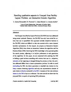
Fig. 3. Comparison of the solution quality (number of correct bits at the end of the run) achieved by the compact GA and the simple GA on a 100-bit onemax problem. The algorithms were ran from population size 4–100 with increments of 2 (4, 6, 8, . . ., 100). The solid line is for the simple GA. The dashed line is for the compact GA.

Fig. 2. Pseudocode of the compact GA.

schema *0** to *1**. The role of the population is to buffer against a finite number of such decision errors. Imagine the following selection scheme: pick two individuals randomly from the population, and keep two copies of the better one. This scheme is equivalent to a steady-state binary tournament selection. In a population of size , the proportion . For instance, in of the winning alleles will increase by the previous example the proportion of 1’s will increase by at gene positions 1 and 3, and the proportion of 0’s will at gene position 2. At gene position 4, also increase by the proportion will remain the same. This thought experiment suggests that an update rule increasing a gene’s proportion simulates a small step in the action of a GA with a by population of size The next section explores how the generation of individuals from a probability distribution mimics the effects of crossover. B. Crossover The role of crossover in the GA is to combine bits and pieces from fit solutions. A repeated application of most commonly used crossover operators eventually leads to a decorrelation of the population’s genes. In this decorrelated state, the population is more compactly represented as a probability vector. Thus the generation of individuals from this vector can be seen as a shortcut to the eventual aim of crossover. Fig. 2 gives pseudocode of the compact GA. C. Two Main Differences from PBIL The proposed algorithm differs from PBIL in two ways: 1) it can simulate a GA with a given population size, and 2) it reduces the memory requirements of the GA.

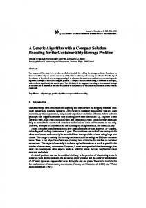
The update step of the compact GA has a constant size . While the simple GA needs to store bits for of each gene position, the compact GA only needs to keep the numbers proportion of ones (and zeros), a finite set of that can be stored with bits. With PBIL’s update rule (see 1), an element in the probability vector can have any arbitrary precision, and the number of values that can be stored in an element of the vector is not finite. Therefore, PBIL cannot achieve the same level of memory compression as the cGA. While in many problems computer memory is not a concern, we can easily imagine large problems that need huge population sizes. In such cases, results cutting down the memory requirement from to in significant savings. PBIL typically generates a large number of individuals from the probability vector. According to Baluja and Caruana [3], that number was something analogous to the population size. In the compact GA, the size of the update step is the “thing” that is analogous to the population size. IV. EXPERIMENTAL RESULTS This section presents simulation results and compares the compact GA with the simple GA, both in terms of solution quality and in the number of function evaluations taken. All experiments are averaged over 50 runs. The simple GA uses binary tournament selection without replacement and uniform crossover with exchange probability 0.5. Mutation is not used and crossover is applied with probability one. All runs end when the population fully converges, that is, when for each gene position all the population members have the same allele value (zero or one). Figs. 3 and 4 show the results of the experiments on a 100-bit onemax problem (the counting ones problem). Fig. 3 plots the solution quality (number of correct bits at the end of the run) for different population sizes. Fig. 4 plots the number of function evaluations taken until convergence for the various population sizes. On both graphs, the solid line is for the simple GA and the dashed line is for the compact GA. Additional simulations were performed with the binary integer function and with De Jong’s test functions [5].

290


Fig. 4. Comparison of the compact GA and the simple GA in the number of function evaluations needed to achieve convergence on a 100-bit onemax problem. The algorithms were ran from population size 4–100 with increments of 2 (4, 6, 8, . . ., 100). The solid line is for the simple GA. The dashed line is for the compact GA.

The results obtained were similar to these, and are collected in Appendix A. The match between the two algorithms seems accurate, and gives evidence that the two are doing roughly the same thing and that they are somehow equivalent. Note however that while the sGA has a memory requirement of bits, the cGA requires only bits. The generation of individuals in the compact GA is equivalent to performing an infinite number of crossover rounds per generation in a simple GA. Thus the compact GA completely decorrelates the genes, while the simple GA still carries a little bit of correlation among the population’s genes. Another difference is that the compact GA is incremental based while the simple GA is generational based. One could get a better approximation of the two algorithms by doing a batch-update competitions are of the probability vector once every performed. This would more closely mimic the generational behavior of the simple GA. We did not do that here because the difference is not significant. We are simply interested in showing that the two algorithms are approximately equivalent.

V. SIMULATING HIGHER SELECTION PRESSURES This section introduces a modification to the compact GA that allows it to simulate higher selection pressures. We would like to simulate a tournament of size . The following mechanism produces such an effect. 1) Generate individuals from the probability vector and find out the best one. 2) Let individuals, the best individual compete with the other updating the probability vector along the way. Clearly, the best individual wins all the competitions, thus the above procedure simulates something like a tournament of size Steps 2–4 of the cGA’s pseudocode (Fig. 2) would have to be replaced by the ones shown in Fig. 5. and Experiments on the onemax problem with are shown in Fig. 6 confirming our expectations. Once more, the graphs show the solution quality and also the number of function evaluations needed to reach convergence. The runs were done for different population sizes. The top graphs are the middle ones for and the bottom ones are for

Fig. 5. Modification of the compact GA that implements tournament selection of size s. This would replace steps 2–4 of the cGA code.

for In all of them, the solid line is for the simple GA and the dashed line is for the compact GA. Being able to simulate higher selection rates should allow the compact GA to solve problems with higher order building blocks in approximately the same way that a simple GA with uniform crossover does. It is known that to solve such problems, high selection rates are needed to compensate for the highly disruptive effects of crossover. Moreover, the population size required to solve such problems grows exponentially with the problem size [19]. To test the compact GA on problems with higher-order building blocks, ten copies of a 3-bit deceptive subfunction are concatenated to form a 30-bit problem. Each subfunction is a 3-bit trap function with deceptive-to-optimal ratio of 0.7 [1], [6]. The results are presented in Fig. 7. In this case there is a discrepancy between the two algorithms. This can be explained on schema theorem grounds. Using uniform crossover, an order- building block has a According to the schema thesurvival probability of orem, the simple GA should be able to propagate these building blocks as long as the selection rate is high enough to compensate for the crossover disruption. For an order-3 schema, the survival probability is 1/4, so the sGA should start to work well when the selection rate is greater than 4. In the case of the cGA, we can think of a global schema theorem. under the cGA would The survival probability of a schema then be given by survival of In the cGA, all the start with 1/2. This means that initially the survival probability of an order-3 building block is 1/8. Therefore, the building block should grow when the selection rate is greater than eight. This argumentation explains the and . results obtained in Fig. 7 (see the cases is not enough to combat Observe that a selection rate of the disruptive effects of crossover. No matter what population size is used, the compact GA (and also the simple GA) with will fail to solve this problem. This is an indication that the problem has higher order building blocks, and that it can only be solved with these kind of algorithms by raising the selection pressure.


291

Fig. 6. The plots illustrate the mapping of the selection rate of the compact GA into that of the simple GA using the onemax function. Selection rates are two, four, and eight. The algorithms were ran from population size 4–100 with increments of two (4, 6, 8, . . . ; 100). For selection rate eight, the initial population size is eight. On the left side, the graphs plot the number of correct bits at the end of the run for the various population sizes. On the right side, the graphs plot the number of function evaluations taken to converge. Selection rates are s = 2 (top), s = 4 (middle), and s = 8 (bottom). The solid lines are for the simple GA, and the dashed lines are for the compact GA.

As mentioned previously, the compact GA completely decorrelates the population’s genes, while the simple GA still carries a little bit of allele correlation. This effect may also help to explain the difference that is observed in the case of the deceptive problem. VI. GETTING MORE

WITH

LESS

This section introduces a concept that is unusual in terms of standard GA practice. To motivate the discussion, let us start with an analogy between the selection operator of a GA and a tennis (or soccer) competition. In tennis there are two kinds of tournaments: elimination and round-robin. In both cases, the players are matched in pairs. In the elimination case, the losers are eliminated from the tournament and the winners proceed to next round. In

the round-robin variation, everybody plays with everybody. It is also possible to have competitions that are something in between these two. An example is the soccer World Cup. There, the teams are divided in groups and within each group the teams play round-robin. Then, the top- within each group proceed to the next phase. After this brief detour, let us shift back to our discussion on genetic algorithms. Typically, a GA using binary tournament selection is very much like an elimination tennis competition. The only difference is that in the GA, each individual participates in two tournaments. This is because we do not want the population to be chopped by a half after each generation. Round-robin competitions are not usually done in GA’s, because this would make the population size grow after each generation.

292


Fig. 7. These plots compare the compact GA and the simple GA on the ten copies of a 3-bit trap function, using selection rates of two, four, and eight. The algorithms were ran for population sizes 8, 500, 1000, 1500, 2000, 2500, and 3000. On the left side, the graphs plot the number of correct building blocks (sub-functions) at the end of the run for the various population sizes. On the right side, the graphs plot the number function evaluations taken to converge. Selection rates are s 2 (top), s = 4 (middle), and s = 8 (bottom). The solid lines are for the simple GA, and the dashed lines are for the compact GA.

=

The remainder of this section shows how it is possible to have round-robin-like competitions within the compact GA while maintaining a fixed population size. To implement it, we do the following: instead of generating two individuals, individuals and make a round-robin tournament generate among them, updating the probability vector along the way. Steps 2–4 of the cGA’s pseudocode (Fig. 2) would have to be replaced by the ones shown in Fig. 8. binary tournaThis results in a faster search because function evaluations. On the ments are made using only other hand, this scheme takes bigger steps in the probability vector and therefore more decision-making mistakes are made. the tournaments are played using elimination. When the tournament is played in a round-robin fashWhen is between ion among all the population members. When 2 and , we get something that is neither a pure elimination scheme nor a pure round-robin scheme.

Fig. 8. Modification of the compact GA that implements a round-robin tournament. This would replace steps 2–4 of the cGA code.

Experiments of the cGA with a selection rate of are performed again, but this time using different values of


Fig. 9. This graph shows the solution quality on a 100-bit onemax problem for various population sizes (4, 6, 8, . . . ; 100), using different values of m: Observe that the solution quality decreases as m increases.

Fig. 10. This graph shows the number of function evaluations needed to reach convergence on a 100-bit onemax problem, using various population sizes (4, 6, 8, . . . ; 100), and different values of m: Observe that the speed increases as m increases.

Plots for the onemax problem are shown in Figs. 9–11. Fig. 9 shows the solution quality (number of correct bits at the end of the run) of the compact GA with for different population sizes. Fig. 10 shows the number of function evaluations taken to converge by the compact GA for the different population sizes. Fig. 11 with is a combination of Figs. 9 and 10. It shows that a given or solution quality can be obtained faster by using instead of . In other words, although using higher reduces the solution quality, the corresponding values of increase in speed makes it worth its while. Observe that after due to solution a certain point, it is risky to increase is worse than degradation. In this example, using or This shows that there must be using and raises important questions concerning GA an optimal efficiency. VII. EXTENSIONS Two extensions are proposed for this work: 1) investigate extensions of the cGA for order- problems and 2) investigate how to maximize the information contained in a finite set of evaluations in order to design more efficient GA’s.

293

Fig. 11. This is a combination of the previous two graphs. It shows that to achieve a given solution quality, it is better to use m = 4 or m = 8 instead of m = 2 or m = 40: In other words, the best strategy is neither to use a pure elimination tournament, nor a pure round-robin tournament.

The compact GA is basically a 1-bit optimizer and ignores the interactions among the genes. The set of problems that can be solved efficiently with such schemes are problems that are somehow easy. The representation of the population in the compact GA explicitly stores all the order-one schemata contained in the population. It is possible to have a similar scheme that is also capable of storing higher order schemata in a compact way. Recently, a number of algorithms have been suggested that are capable of dealing with pairwise gene interactions [4], [7], [16] and even with order- interactions [11], [17]. Another direction is to investigate more deeply the results discussed in Section VI and discover their implications for the design of more efficient GA’s. Our preliminary work has shown that it is possible to extract more information from a set of function evaluations, than the usual information extracted by the simple GA. But how to use this additional information in the context of a simple GA is still an open question and deserves further research. VIII. CONCLUSIONS This paper presented the compact GA, an algorithm that mimics the order-one behavior of a simple GA with a given population size and selection rate, but that reduces its memory requirements. The design of the compact GA was explained, and computational experiments illustrated the approximate equivalence of the compact GA with a simple GA using uniform crossover. Although the compact GA approximately mimics the orderone behavior of the simple GA with uniform crossover, it is not a replacement for the simple GA. Simple GA’s can perform quite well when the user has some knowledge about the nonlinearities in the problem. In that case, the building blocks can be tightly coded and they can be propagated throughout the population through the repeated action of selection and recombination. Note that in general, this linkage information is not known. In most applications, however, the GA user has some knowledge about the problem’s domain and tends to code together in the chromosome features that are somehow spatially related in the original problem. In a way, the GA

294


(a)

(a)

(b)

(b)

Fig. 12. Comparison of the simple GA and the compact GA on a 30-bit binary integer function. (a) shows the solution quality obtained at the end of the runs. (b) shows the number of function evaluations taken to converge. The algorithms were ran from population size 4–140 with increments of two (4, 6, 8, . . . ; 140). The solid line is for the simple GA and the dashed line is for the compact GA.

Fig. 13. Comparison of the simple GA and the compact GA on function F1. (a) shows the solution quality obtained at the end of the runs. (b) shows the number of function evaluations taken to converge. The algorithms were ran from population size 4–100 with increments of two (4, 6, 8, . . . ; 100). The solid line is for the simple GA and the dashed line is for the compact GA.

user has partial knowledge about the linkage. This is probably one of the main reasons why simple GA’s have had so much success in real-world applications. Of course, sometimes the user think he has a good coding, when in fact he does not. In such cases, simple GA’s are likely to perform poorly. Finally, and most important, this study has introduced new ideas that have important ramifications for GA design. By looking at the simple GA from a different perspective, we learned more about its complex dynamics and opened new doors toward the goal of having more efficient GA’s.

First it pays attention to the most significant bits and then, once those bits have converged, it moves on to next most significant bits. For this function, the solution quality is measured by the number of consecutive bits solved correctly. For De Jong’s test functions, the solution quality is measured by the objective function value obtained at the end of the run. Each parameter is coded with the same precision as described in his dissertation [5]. The functions F1–F5 are shown below. De Jong’s F1:

APPENDIX A This appendix presents simulation results comparing the compact GA and the simple GA on the binary integer function, and on De Jong’s test functions [5]. All experiments are averaged over 50 runs. The simple GA uses binary tournament selection without replacement and uniform crossover with exchange probability 0.5. Mutation is not used, and crossover is applied all the time. All runs end when the population fully converges—that is—when all the individuals have the same alleles at each gene position. The binary integer function is defined as The GA solves this problem in a sequential way (domino-like).

De Jong’s F2:

De Jong’s F3: integer


295

(a)

(a)

(b)

(b)



De Jong’s F4: Gauss De Jong’s F5:

quently, the convergence process starts to look like a randomwalk. The drift time is slightly longer in the case of the simple GA, however, possibly because the simple GA uses tournament selection without replacement, while the compact GA does something more similar to tournament with replacement. The important thing to retain is that the behavior of compact GA is approximately equivalent to that of the simple GA. APPENDIX B PHYSICAL INTERPRETATION

Figs. 12–17 illustrate the comparison between the compact GA and the simple GA on the binary integer function and on De Jong’s test functions. In functions F3 and F4, the number of function evaluations needed to reach convergence by the two algorithms do not match very closely. F3 has many optima, and F4 is a noisy fitness function. Due to the effects of genetic drift, it takes a long time for both algorithms to fully converge. Genetic drift occurs when there is no selection pressure to distinguish between two or more individuals, and conse-

An analogy with a potential field can be made to explain the search process of the compact GA and is easily visualized for 2-bit problems. Similar results were obtained in [13] in the context of studying the convergence behavior of the PBIL algorithm. For completeness, they are presented again. Consider Fig. 18. The corner points are the four points of the search space (00, 01, 10, 11). Each corner point applies a force to attract the particle (population) represented by the , which black dot. The position of the particle is given by represents the proportion of 1’s in the first and second gene positions respectively. The particle (population) is submitted

296


(a)

(a)

(b)

(b)



to a potential field on the search space, seeking its minimum. As the search progresses, the particle (population) moves up or down, left or right (the proportions of 1’s in each gene ) and eventually, one of the corners increase or decrease by will capture the particle (the population converges). Let us illustrate this with a 2-bit onemax problem and with the minimal deceptive problem (MDP) [9]. Onemax Let and be the proportion of 1’s at the first and second genes respectively. The search space, the potential field, and a graphical interpretation is shown as point fitness

Fig. 18. The black circle represents the population. Its coordinates are p and q , the proportion of 1’s in the first and second gene positions. The four corners are the points in the search space.

MDP Likewise, for the minimal deceptive problem, the search space is point fitness

The potential at position

is:


297

REFERENCES

Fig. 19.

Potential field for the 2-bit onemax problem.

Fig. 20.

Potential field for the MDP.

and the potential at position

is

Fig. 19 shows that the onemax is an easy function. Fig. 20 gives a visual representation of Goldberg’s observation [9] that on the MDP, the GA could converge to the deceptive attractor given certain initial conditions (high proportion of 00 in the initial population).

[1] D. H. Ackley, A Connectionist Machine for Genetic Hill Climbing. Boston, MA: Kluwer, 1987. [2] S. Baluja, “Population-based incremental learning: A method for integrating genetic search based function optimization and competitive learning,” Carnegie Mellon Univ., Pittsburgh, PA, Tech. Rep. CMUCS-94-163, 1994. [3] S. Baluja and R. Caruana, “Removing the genetics from the standard genetic algorithm,” Carnegie Mellon Univ., Pittsburgh, PA, Tech. Rep. CMU-CS-95-141, 1995. [4] S. Baluja and S. Davies, “Using optimal dependency-trees for combinatorial optimization: Learning the structure of the search space,” in Proc. 14th Int. Conf. Machine Learning. San Mateo, CA: Morgan Kaufmann, 1997, pp. 30–38. [5] K. A. De Jong, “An analysis of the behavior of a class of genetic adaptive systems,” Ph.D. dissertation, Univ. Michigan, Ann Arbor, 1975. [6] K. Deb and D. E. Goldberg, “Analyzing deception in trap functions,” in Foundations of Genetic Algorithms 2, L. D. Whitley, Ed. San Mateo, CA: Morgan Kaufmann, 1993, pp. 93–108. [7] J. S. De Bonet, C. Isbell, and P. Viola, “MIMIC: Finding optima by estimating probability densities,” in Advances in Neural Information Processing Systems, M. C. Mozer, M. I. Jordan, and T. Petsche, Eds. Cambridge, MA: MIT Press, vol. 9, p. 424, 1997. [8] L. J. Eshelman and J. D. Schaffer, “Crossover’s niche,” in Proc. 5th Int. Conf. Genetic Algorithms, S. Forrest, Ed. San Mateo, CA: Morgan Kaufmann, 1993, pp. 9–14. [9] D. E. Goldberg, “Simple genetic algorithms and the minimal, deceptive problem,” in Genetic Algorithms and Simulated Annealing, L. Davis, Ed. San Mateo, CA: Morgan Kaufmann, 1987, pp. 74–88. [10] G. Harik, E. Cantú-Paz, D. E. Goldberg, and B. Miller, “The gambler’s ruin problem, genetic algorithms, and the sizing of populations,” in Proc. 4th Int. Conf. Evolutionary Computation, T. Bäck, Ed. Piscataway, NJ: IEEE Press, 1997, pp. 7–12. [11] G. Harik, “Linkage learning via probabilistic modeling in the ECGA,” Univ. Illinois, Urbana-Champaign, IlliGAL Rep. 99010, 1999. [12] J. Hertz, A. Krogh, and G. Palmer, Introduction to the Theory of Neural Computation. Reading, MA: Addison-Wesley, 1993. [13] M. Höhfeld and G. Rudolph, “Toward a theory of population-based incremental learning,” in Proc. 4th Int. Conf. Evolutionary Computation, T. Bäck, Ed. Piscataway, NJ: IEEE Press, 1997, pp. 1–5. [14] H. Kargupta and D. E. Goldberg, “SEARCH, blackbox optimization, and sample complexity,” in Foundations of Genetic Algorithms 4, R. K. Belew and M. D. Vose, Eds. San Francisco, CA: Morgan Kaufmann, 1996, pp. 291–324. [15] H. Mühlenbein and G. Paaß, “From recombination of genes to the estimation of distributions I. binary parameters,” in Parallel Problem Solving from Nature, PPSN IV, H.-M. Voigt, W. Ebeling, I. Rechenberg, and H.-P. Schwefel, Eds. Berlin, Germany: Springer-Verlag, 1996, pp. 178–187. [16] M. Pelikan and H. Mühlenbein, “The bivariate marginal distribution algorithm,” in Advances in Soft Computing—Engineering Design and Manufacturing, R. Roy, T. Furuhashi, and P. K. Chawdhry, Eds. Berlin, Germany: Springer-Verlag, 1999, pp. 521–535. [17] M. Pelikan, D. E. Goldberg, and E. Cantú-Paz, “BOA: The Bayesian optimization algorithm,” Univ. Illinois, Urbana-Champaign, IlliGAL Rep. 99003, 1999. [18] G. Syswerda, “Simulated crossover in genetic algorithms,” in Foundations of Genetic Algorithms 2, L. D. Whitley, Ed. San Mateo, CA: Morgan Kaufmann, 1993, pp. 239–255. [19] D. Thierens, and D. E. Goldberg, “Mixing in genetic algorithms,” in Proc. 5th Int. Conf. Genetic Algorithms, S. Forrest, Ed. San Mateo, CA: Morgan Kaufmann, 1993, pp. 38–45.