In this paper we consider the problem of testing for a parameter change in regression models with ARCH errors based on the residual cusum test. It is shown.
J. Japan Statist. Soc. Vol. 34 No. 2 2004 173–188
THE CUSUM TEST FOR PARAMETER CHANGE IN REGRESSION MODELS WITH ARCH ERRORS Sangyeol Lee*, Yasuyoshi Tokutsu** and Koichi Maekawa*** In this paper we consider the problem of testing for a parameter change in regression models with ARCH errors based on the residual cusum test. It is shown that the limiting distribution of the residual cusum test statistic is the sup of a Brownian bridge. Through a simulation study, it is demonstrated that the proposed test circumvents the drawbacks of Kim et al.’s (2000) cusum test. For illustration, we apply the residual cusum test to the return of yen/dollar exchange rate data. Key words and phrases: Brownian bridge, regression models with ARCH errors, residual cusum test, test for parameter change, weak convergence.
1. Introduction Since Page (1955), the problem of testing for a parameter change has been an important issue in statistics. It first started in the quality control context and quickly moved to other fields such as economics, engineering and medicine. So far, a large number of articles have been published in various journals. See, for instance, Brown et al. (1975), Wichern et al. (1976), Zacks (1983), Krishnaiah and Miao (1988) and Cs¨ org˝ o and Horv´ ath (1997). The change point problem has drawn much attention from many researchers in time series analysis since time series often suffer from structural changes owing to changes of policy and critical social events. It is well known that detecting a change point is a crucial task and ignoring it can lead to a false conclusion. A standard example can be found in Hamilton ((1994), p. 450). For relevant references, we refer to Wichern et al. (1976), Picard (1985), Incl´ an and Tiao (1994), Mikosch and St˘ aric˘ a (1999), Lee and Park (2001), Lee et al. (2003a, b) and the papers cited in those articles. In this paper, we concentrate ourselves on Incl´ an and Tiao’s (1994) cusum test in regression models with ARCH errors. The ARCH and GARCH models have long been popular in financial time series analysis. For a general review, see Gouri´eroux (1997). Incl´ an and Tiao’s (1994) cusum test was originally designed for testing for variance changes and allocating their locations in iid samples. Later, it was demonstrated that the same idea can be extended to a large class of time series models (cf., Lee et al. (2003a)). Also, the variance change test has been studied in unstable AR models (cf., Lee et al. (2003b)). In fact, Kim et al. (2000) considered to apply the cusum test to GARCH(1, 1) Received December 2, 2003. Revised May 29, 2004. Accepted June 9, 2004. *Department of Statistics, Seoul National University, Seoul 151-742, Korea. **Center for Research on Regional Economic Systems, Hiroshima University, Hiroshima 730-0053, Japan. ***Faculty of Economics, Hiroshima University, Hiroshima 739-8525, Japan.
174
SANGYEOL LEE ET AL.
models taking account of the fact that the variance is a functional of GARCH parameters, and their change can be detected by examining the existence of the variance change. Although this reasoning was correct, it turned out that the cusum test suffers from severe size distortions and low powers. Hence, there was a demand to improve their cusum test. Here, in order to circumvent such drawbacks, we propose to use the cusum test based on the residuals, given as the squares of observations divided by estimated conditional variances. We intend to use residuals since the residual based test conventionally discard correlation effects and enhance the performance of the test. In fact, a significant improvement was observed in our simulation study. Despite the previous work of Lee et al. (2003b) also considers a residual cusum test in time series models, the model of main concern was the autoregressive model with several unit roots. In fact, the mathematical analysis of the cusum test heavily relies on the probabilistic structure of the underlying time series model, and the arguments used for establishing the weak convergence result for unstable models are somewhat different from those for ARCH models. Therefore it is worth to investigate the asymptotic behavior of the residual cusum test in ARCH models. Although the present paper was originally motivated to improve Kim et al.’s (2000) test in the GARCH(1, 1) model, we consider the cusum test in a more general class of models including regression models with infinite order ARCH errors. The organization of this paper is as follows. In Section 2, we introduce the residual cusum test in regression models with infinite order ARCH models that include the GARCH model, and show that its limiting distribution is the sup of a Brownian bridge. In Section 3, we perform a simulation study to compare our test with Kim et al.’s (2000) test in GARCH(1, 1) models. The result indicates that our method outperforms their cusum test. Then, for illustration, we apply our test to a real data set. Finally, in Section 4, we provide concluding remarks. 2. Residual cusum test Let us consider the model (2.1)
yt = β � z t + �t , �t = ht ξt , h2t
= a(θ) +
∞ �
bj (θ)�2t−j ,
j=1
where ξt are iid r.v.’s with zero mean and unit variance, {z t } is a p-dimensional strictly stationary process, and θ → a(θ) and θ → b(θ) are nonnegative continu�∞ d ous real functions defined on a subset N in R with a(θ) > 0 and j=1 bj (θ) < ∞ for all θ ∈ N . We assume that ys , z s , s < t are independent of ξu , u ≥ t, and {(�t , ht , z t )} is strong mixing. The Model (2.1) covers a broad class of important models in the financial time series context including GARCH models. In particular, it becomes a GARCH(1, 1) model if we put z t = 0, θ = (ω, α1 , α2 ), ω >
THE CUSUM TEST FOR PARAMETER CHANGE IN REGRESSION
175
0, α1 , α2 ≥ 0, α1 + α2 < 1, a(θ) = ω/(1 − α1 − α2 ) and bj (θ) = α1 α2j−1 . In this case, {(�t , ht , z t )} is geometrically strong mixing (cf., Carrasco and Chen (2002)). Recently, Lee and Taniguchi (2004) studied the LAN property and the residual empirical process for Model (2.1). The objective here is to test the hypotheses H0 : η = (β � , θ � )� remains the same for the whole series vs. H1 : Not H0 . �
� z t } as For a test, one may construct a cusum test based on {ˆ εt := yt − β in Incl´ an and Tiao (1994) and Kim et al. (2000). However, as observed in the simulation study in Section 3, the test in GARCH(1, 1) models is unstable and produces low powers. Thus one has to develop a better test which is not much affected by the GARCH parameters. As a candidate, one can naturally consider � 2� the cusum test based on ξt , say, � � � � k n �� � 1 k � � ξt2 − ξt2 � , max � Tn := √ � n nτ 1≤k≤n � t=1 t=1 where τ 2 = Var(ξ12 ), since Tn is free from the GARCH parameters. In this case, however, one may speculate whether Tn can detect any changes since Tn itself has no information about the GARCH parameters. But since ξt are not observable, one should replace ξt2 ’s by the residuals ξˆt2 , which are obtained via estimating the unknown parameters. Those estimators play an important role to detect changes in the parameters in the presence of changes, while the iid property of the true errors still remains when there are no changes. From this reasoning, one can anticipate that the residual cusum test should be more stable and produce better powers. Now, we construct the residual cusum test. To this end, we assume that (A1) E z 1 4+δ1 < ∞, E|�1 |4+δ1 < ∞ and E|ξ1 |4+δ1 < ∞ for some δ1 > 0. (A2) There exists δ2 > 0 such that sup
�θ−θ� �≤δ2 ,θ� ∈N
a(θ) ˙
< ∞
and
∞ �
sup
� � j=1 �θ−θ �≤δ2 ,θ ∈N
b˙j (θ) < ∞,
where a(θ) ˙ and b˙ j (θ) denote the gradient vectors of a and bj at θ. √ (A3) There exists a sequence of positive integers with q → ∞, q/ n → 0 and √ �∞ n j=q+1 bj (θ) → 0 as n → ∞. δ1 � 4+δ1 < (A4) {(�t , ht , z t )} is strong mixing with order γ(h) satisfying ∞ h=1 γ(h) ∞. Observe that the last condition in (A3) is satisfied if bj (θ) are geometrically bounded (as in GARCH models), and q = [(log n)]ζ , ζ > 1. Also, if z t are identically zero and {yt } is a GARCH process, {(yt , ht )} is geometrically strong mixing (cf., Carrasco and Chen (2002)), so that (A4) is satisfied.
176
SANGYEOL LEE ET AL.
Now, we construct the residual cusum test. In analogy of h2t , we define h2t
� + = a(θ)
q �
� �2 , bj (θ)� t−j
j=1 �
� zt � �t = yt − θ �
�
and ξ�t = � �t /� ht ,
� ,θ � )� is an estimator of η with � = (β where η the following result.
√
n(� η − η) = OP (1). Then, we have
Theorem 1. Assume that (A1)–(A4) hold. Set � � � � � � � k n � � 1 k 2 2� � � � � ξt − ξt � Tn := √ max � n n� τ q+1≤k≤n �t=q+1 t=q+1 � where τ�2 =
1 n−q
�n
�4 t=q+1 ξt
1 − ( n−q
�n
�2 2 t=q+1 ξt ) .
d T�n −→ sup |B o (u)|, 0≤u≤1
Then, under H0 , n → ∞,
where B o is a Brownian bridge. Remark 1. A choice of q may be an issue in actual practice since it may affect the test, despite the affection would not be so serious for fairly large samples. However, if h2t has a more specific form as in GARCH(1, 1) models, the test statistic can be free of the choice of q. See Theorem 2 below. In general, the above Brownian bridge result does not hold for all regression models (cf., Jandhyala and MacNeill (1991)). Therefore, the result of Theorem 1 should not be applied directly to all situations. � Proof. Split ξ�t2 into ξt2 + 6i=1 Ji,t , where J1,t = J3,t J5,t
h2t )ξt2 (h2t − � , h2t
� − β)� z t �t −2(β = , h2t � − β)� z t �t (h2 − � h2t )2 −2(β t = , h2t h4t �
J2,t =
h2t )2 ξt2 (h2t − � , h2 h2 � t t
J4,t J6,t
� − β)� z t �t (h2 − � h2t ) −2(β t = , h4t � − β)� z t )2 ((β = . � h2t
We claim that (2.2) ∆i,n
� � � � � � � k n � � 1 k � := √ Ji,t − Ji,t �� = oP (1), max � n n q+1≤k≤n �t=q+1 � t=q+1
i = 1, . . . , 6.
THE CUSUM TEST FOR PARAMETER CHANGE IN REGRESSION
177
First, we handle J1,t . Note that � + h2t − � h2t =a(θ) − a(θ)
∞ �
bj (θ)�2t−j
j=q+1
(2.3)
+
q
�
q 4 � � �
2 2 � �2 + � := bj (θ) − bj (θ) b ( θ) � − � � Ii,t . j t−j t−j t−j
j=1
j=1
i=1
Owing to (A4) and the invariance principle for strong mixing processes (cf., Theorem 1.7 of Peligrad (1986)), we have � � � � � 2 � � � k n � 2 2 2 � ξt k ξt 1 ξ ξ � √ − E t2 − − E t2 �� = OP (1), max �� 2 2 n n q+1≤k≤n �t=q+1 ht ht ht ht � t=q+1 which implies (2.4)
� � � � � � � n 2� � k I1,t ξt2 I ξ k 1 1,t t � � √ − max = oP (1). n n q+1≤k≤n ��t=q+1 h2t h2t �� t=q+1
Meanwhile, (2.5)
� � � � � � � k n 2 2 � � I ξ I ξ k 1 2,t 2,t t t � = oP (1) √ − max �� � 2 2 n n q+1≤k≤n �t=q+1 ht h � t t=q+1
since by (A3), 1 √ n
n �
∞ �
�2t−j ξt2 bj (θ) 2 ht t=q+1 j=q+1
√ = OP n
∞ �
bj (θ) = oP (1).
j=q+1
Now, we verify that (2.6)
� � � � � � � k n 2 2 � I3,t ξt I3,t ξt �� k 1 � √ = oP (1). − max n n q+1≤k≤n ��t=q+1 h2t h2t �� t=q+1
For this task, it suffices to show that for λ > 0, q � � n > λ = o(1), (2.7) |bj (θ) − bj (θ)|Λ ln := P j
n → ∞,
j=1
where Λnj
� � ��� � � � k �2t−j ξt2 � �2t−j ξt2 1 � =√ −E max � � n q+1≤k≤n ��t=q+1 h2t h2t �
178
SANGYEOL LEE ET AL.
which is OP (1) due to the invariance principle and (A4). Observe that for any M > 0, M ∞ � � � n > λ + P � n > λ |bj (θ) − bj (θ)|Λ |bj (θ) − bj (θ)|Λ ln :≤ P j j 2 2 j=1
j=M +1
:= l1,n + l2,n , l1,n = o(1), and � �−θ
l2,n ≤ P θ ∞ �
×
j=M +1
˙ � ) · √1 sup b(θ n �θ−θ� �≤δ2
� n � �2t−j ξt2 t=1
h2t
+
n �
E
t=1
�2t−j ξt2
�
h2t
λ > 2
�
for all large n. Then, using Markov’s inequality and (A2), we can show that l2,n becomes arbitrarily small by taking a sufficiently large M . Hence, l2,n = o(1) and thus ln = o(1), which yields (2.6). Now, we verify that � � � � � � � n n 2 2 � I4,t ξt I4,t ξt �� 1 k � √ = oP (1). (2.8) − max n n q+1≤k≤n ��t=q+1 h2t h2t �� t=q+1 Note that � − β)� z t−j − ((β � − β)� z t−j )2 . �2t−j = 2�t−j (β �2t−j − � Since
� � � � � n � 2 2 � z t−j �t−j ξt z t−j �t−j ξt � 1 � = OP (1) √ − E max � � n q+1≤k≤n � h2t h2t �t=q+1 �
by (A4), and ∞ � j=1
(2.9)
� ≤ bj (θ)
∞ �
� − θ
θ
j=1
sup � −θ� �θ−θ� �≤�θ
∞ � � �˙ � � � bj (θ) �bj (θ )� + j=1
= OP (1),
following essentially the same arguments between (2.6) and (2.8), we can see that � � � q 2 � k � 1 � β � − β)� z t−j �t−j ξt � √ bj (θ)( max � n q+1≤k≤n �t=q+1 h2t j=1 � � � � q n � 2 � k � z t−j �t−j ξt � � � (2.10) − bj (θ)(β − β) � = oP (1). 2 n ht � t=q+1 j=1
THE CUSUM TEST FOR PARAMETER CHANGE IN REGRESSION
179
Combining this and the fact that q n 1 � � � � √ bj (θ) β − β 2 z t−j 2 ξt2 /h2t = oP (1), n t=q+1
(by (2.9))
j=1
we obtain (2.8). From (2.4), (2.5), (2.6) and (2.8), we establish ∆1,n = oP (1). � to show h2t ≥ a(θ), Now, we deal with ∆2,n . Since h2t ≥ a(θ) > 0 and � � n 1 √ t=q+1 J2,t = oP (1), it suffices to prove n n 1 � 2 �2 2 2 √ (h − ht ) ξt = oP (1). n t=q+1 t
(2.11) It is obvious that
√1 n
�n
2 2 t=q+1 I1,t ξt
n �
(2.12)
= oP (1). Also, we have n �
∞ �
2
1 1 2 2 √ I2,t ξt = √ bj (θ)�2t−j ξt2 n t=q+1 n t=q+1 j=q+1 2 ∞ � √ = OP n bj (θ) = oP (1) j=q+1
by (A3). Meanwhile, by the Cauchy-Schwarz inequality, q n n � � 1 � � � 1 � 2 2 � ˙ � �2 4 4 √ I3,t ξt ≤ √
θ − θ 2 sup �bj (θ )� �t−j ξt n t=q+1 n t=q+1 � −θ� �θ−θ� �≤�θ j=1 √ (2.13) = OP (q/ n) = oP (1). (by (A3))
Moreover, n �
n �
2 1 2 2 √ I4,t ξt ≤ √ n t=q+1 n t=q+1 (2.14)
2 q � � − β)� z t−j | + ((β � − β)� z t−j )2 } ξ 2 bj (θ){|�t−j (β t j=1
= oP (1).
This together with (2.11)–(2.13) yields ∆2,n = oP (1). Now, it remains to show that ∆n,i = oP (1), i = 3, 4, 5, 6. It is trivial to show that ∆n,3 = oP (1) and ∆n,6 = oP (1). Also, one can verify the negligibility of ∆n,4 and ∆n,5 in a similar fashion to prove that of ∆n,1 and ∆n,2 , respectively. Hence, (2.2) is established, which directly implies � � � � � � � k n � � 1 k 2 2� � � � √ ξt − ξt � max � n n q+1≤k≤n �t=q+1 t=q+1 � � � � � � � � k n � � k 1 2 2� � =√ (2.15) ξt − ξt � + oP (1). max � n n q+1≤k≤n �t=q+1 t=q+1 �
180
SANGYEOL LEE ET AL. P
Finally, we show that τ�2 −→ τ 2 = Var(ξ12 ). Note that ˆ 2 )ξ 2 (h2 − h t t ξ�t2 − ξt2 = t + ρt , 2 � ht
(2.16)
ε2t − ε2t )/� h2t satisfies where ρt := (� n 1 � ρt = oP (1) n
(2.17)
and
t=q+1
n 1 � 2 ρt = oP (1). n t=q+1
Thus, in view of (2.11) and (2.17), � � � � � � � � � n n n 2 2 2 � �1 � � 1 � � � (h − h )ξ (� h2t − h2t )2 ξt2 1 t t t 2 2 � − ξ )� ≤ � � � + ( ξ + oP (1) t t � �n � �n 2 ht h2t h2t � � � n � � t=q+1
t=q+1
t=q+1
1/2
n 1 � 2 �2 2 ≤ a(θ) (ht − ht ) n t=q+1
1/2 n � 1 ξt4 + oP (1), n t=q+1
which is oP (1) since (2.11) with ξt2 replaced by 1 is also oP (1), of which proof is essentially the same as that of (2.11) and is omitted for brevity. Hence, n � 1 P ξ�t2 −→ Eξ12 . n−q
(2.18)
t=q+1
Now, by (2.17), n n 1 � �2 1 � 2 �2 2 4 � 2 2 2 (ξt − ξt ) ≤ (ht − ht ) ξt /a(θ) + oP (1) n n t=q+1 t=q+1 � � n � 1 1 � 2 + oP (1) ≤ √ (h2t − � h2t )2 ξt2 a(θ) max ξt2 √ n q+1≤t≤n n t=q+1
= oP (1), and furthermore, n n n 1 � �2 2 � �2 8 � 4 2 2 2 2 (ξt + ξt ) ≤ (ξt − ξt ) + ξt = OP (1). n n n t=q+1
t=q+1
t=q+1
Hence, � � 1/2 1/2 � � n n n n � � � �1 � � 1 1 1 � ξ�t4 − ξt4 �� ≤ (ξ�t2 − ξt2 )2 (ξ�t2 + ξt2 )2 �n n n n � t=q+1 t=q+1 � t=q+1 t=q+1 = oP (1),
THE CUSUM TEST FOR PARAMETER CHANGE IN REGRESSION
181
� P P so that (n − q)−1 nt=q+1 ξ�t4 → Eξ14 . This together with (2.18) yields τ�2 −→ τ 2 . In view of this and (2.15), we establish the theorem. � Now, as mentioned in the remark below Theorem 1, we demonstrate that a modification of the test, free from a choice of q, can be constructed for the models with h2t satisfying a specific equation. Here, considering its extreme popularity in the financial time series context, we concentrate ourselves on the case of GARCH(1, 1) errors: (2.19)
yt = β � z t + εt , εt = ht ξt , h2t = ω + α1 ε2t−1 + α2 h2t−1
with ω > 0, α1 , α2 ≥ 0 and α1 + α2 < 1. In this case, we can write (2.20)
h2t
= a + α1
∞ �
α2j−1 ε2t−j
j=1
with a = ω/(1 − α1 − α2 ), and its estimate is (2.21)
� h2t = � a+α �1
q �
α �2j−1 ε�2t−j ,
j=1
� � z t , β, � � a, α �1 , α �2 are the estimators for β, a, α1 and α2 satisfying where ε�t = yt − β √ √ � − β) = OP (1), n(β n(� a − a) = OP (1), √ √ n(� α1 − α1 ) = OP (1) and n(� α2 − α2 ) = OP (1), √ √ and q is a sequence of positive integers with q → ∞, q/ n → 0 and nα2q → 0, which ensures (A3). Note that the estimate of the conditional variance can be obtained recursively from the equation (2.22)
˜2 = ω ˜2 , h �+α �1 ε�2t−1 + α �2 h t t−1
˜ 2 are provided. From this, we have that for in so far as initial values ε�20 and h 0 t ≥ 2, (2.23)
˜2 = ω h � (� α2t − 1)/(1 − α �2 ) + α �1 t
t−1 �
˜ 2. α �2j−1 ε�2t−j + α �1 α �2t−1 ε�20 + α �2t h 0
j=1
Then, in view of (2.21) and (2.23), we have (2.24)
n 1 � 2 � −2 ˜ −2 √ ε� |h − ht | = oP (1), n t=q+1 t t
182
SANGYEOL LEE ET AL.
and moreover, √ 1 � 2 � −2 ˜ −2 √ εˆt |ht − ht | = OP (q/ n) = oP (1). n t=1 q
(2.25)
Therefore, from Theorem 1, (2.24) and (2.25), we have the following. ˜ 2 be the one in (2.22), and set ξ˜2 = ε�2 /h ˜ 2 . Let Theorem 2. Let h t t t t � k � � � n �� � 1 k � � 2 ˜ ˜ ˜ ξt − ξ˜t2 � , Tn := max Tn,k := √ max � � 1≤k≤n n n˜ τ 1≤k≤n � t=1
where τ˜2 =
1 n
�n
˜4 t=1 ξt
− ( n1
�n
˜2 2 t=1 ξt ) .
Then if (A1) holds, under H0 ,
d T˜n → sup |B o (u)| , 0≤u≤1
t=1
n → ∞.
Remark 2. Notice that unlike in T�n , the first q number of T˜n,k ’s are involved in construction of T˜n . Therefore the test statistic is free from a choice of q in ˜ 2 , one can put any numbers. However, this sense. As for initial values ε˜20 and h 0 � �2 ˜ 2 = 1 �n one may like to choose ε˜20 = n1 nt=1 ε�2t and h 0 t=q+1 ht . In the latter, n−q a choice of q is not a serious concern since initial effects somehow will disappear very fast. It may be reasoned that the initial values may affect the test, but the effect will not be severe since the last two terms in (2.23) decay to 0 exponentially fast. In the case of z t = (yt−1 , . . . , yt−p+1 )� , one� has to adopt the test T˜p,n := 1 2 ˜ maxp+1≤k≤n Tn,k and the initial value ε˜p,0 = n−p nt=p+1 ε�2t . 3. Empirical study 3.1. Simulation study In this section, we evaluate the performance of the test statistic T˜n through a simulation study. Towards this end, we introduce the model yt = ht ξt , 2 h2t = ω + α1 yt−1 + α2 h2t−1 ,
where y0 is assumed to be 0 and {ξt } are iid standard normal random variables. In order to see the power, we consider the following hypotheses: H0 : θ = (ω, α1 , α2 ) are constant during the time t = 1, . . . , n. vs. H1 : θ changes to θ� = (ω � , α1� , α2� ) at n/2. ˜ 2 and q = [(log n)2 ], for the sample size n = Here we evaluate T˜n , with ε˜20 , h 0 500, 800, 1000. In particular, the T˜n is compared with Kim et al.’s (2000) test ˆ In this simulation we perform the test at a nominal level 0.05. statistic BT (C).
THE CUSUM TEST FOR PARAMETER CHANGE IN REGRESSION
183
The empirical sizes and power are calculated as the rejection number of the null hypothesis out of 1000 iterations, and are summarized in Tables 1–3. The figures in the parentheses denote the sizes and powers of Kim et al.’s test. As we see in the tables, our test has no severe size distortions. In particular, the test is still stable even for the case that α1 + α2 is close to 1 (see Tables 2 and 3). As mentioned earlier, this is because ξ�t2 behaves asymptotically like iid ξt2 , unaffected by the GARCH parameters. Meanwhile, we can see that the powers are more than 0.9 at the sample size = 1000. In general, the cusum test in GARCH models requires a much larger sample size to make accurate inferences compared to iid samples. It seems that the GARCH data with volatility makes it harder to identify small changes. Compared to ours, Kim et al.’s test has severe size distortions and much lower powers. Although we do not report details here, we also evaluated the test Tˆn with q = [(log n)3/2 ], [(log n)2 ] and [(log n)3 ]. As a result, we could see that the performance of the tests with q = [(log n)3/2 ] and q = [(log n)2 ] is almost the same as the T˜n , but Tˆn with q = [(log n)3 ] performs poorly compared to the others. Actually, there is no way to choose the most optimal q. We recommend to use [(log n)2 ] since it consistently gives good results in our simulation study. Table 1. θ = (0.5, 0.2, 0.2). θ� = (ω � , α� , β � )
n = 500
n = 800
n = 1000
n = 1500
Size
0.026 (0.020)
0.033 (0.025)
0.049 (0.035)
0.043 (0.039)
(3.0, 0.2, 0.2)
0.306 (0.077)
0.866 (0.031)
0.990 (0.009)
(0.5, 0.6, 0.2)
0.493 (0.144)
0.777 (0.349)
0.901 (0.432)
(0.5, 0.2, 0.6)
0.537 (0.111)
0.806 (0.269)
0.902 (0.381)
Table 2. θ = (0.1, 0.4, 0.4). θ� = (ω � , α� , β � )
n = 500
n = 800
n = 1000
n = 1500
Size
0.036 (0.009)
0.038 (0.004)
0.049 (0.005)
0.040 (0.002)
(0.4, 0.4, 0.4)
0.854 (0.198)
0.994 (0.387)
0.997 (0.449)
(0.1, 0.1, 0.4)
0.526 (0.157)
0.839 (0.493)
0.928 (0.646)
Table 3. θ = (0.1, 0.2, 0.7). θ� = (ω � , α� , β � )
n = 500
n = 800
n = 1000
n = 1500
Size
0.020 (0.002)
0.032 (0.003)
0.032 (0.008)
0.042 (0.010)
(0.4, 0.2, 0.7)
0.219 (0.173)
0.722 (0.228)
0.919 (0.271)
(0.1, 0.2, 0.2)
0.616 (0.070)
0.917 (0.194)
0.983 (0.313)
Next we show an example of the simulated distribution for a estimated break point obtained by T˜n , viz, the estimator of break point is the k maximizing T˜n,k in Theorem 2. For this task, we consider the time series that have only one structural break point in the middle of the series, i.e., θ = (0.1, 0.4, 0.4) in the first sample period is changed to θ� = (0.4, 0.4, 0.4) in the second sample period. Figures 1–3 show the distribution of estimated break points for the sample sizes
184
SANGYEOL LEE ET AL.
300
250
200
150
100
50
0 180
190
200
210
220
230
240
250
260
270
280
290
300
310
320
330
340
Figure 1. Estimated break point: n = 500.
300
250
200
150
100
50
0 305 315 325 335 345 355 365 375 385 395 405 415 425 435 445 455 465 475 485 495 505
Figure 2. Estimated break point: n = 800.
300
250
200
150
100
50
0 390 400 410 420 430 440 450 460 470 480 490 500 510 520 530 540 550 560 570 580 590 600 610
Figure 3. Estimated break point: n = 1000.
THE CUSUM TEST FOR PARAMETER CHANGE IN REGRESSION
185
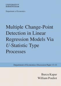
n = 500, 800, 1000, respectively. The number of iterations is 1000 for all cases. The figures indicate that the simulated distributions have a bell shape and are symmetric about the change point. The result demonstrates the validity of the estimator. Overall, our simulation study strongly supports that the residual cusum test performs adequately. 3.2. Real data analysis In this section, we intend to demonstrate the validity of our method in actual practice. For this task, we analyze the return of yen/dollar exchange rate data from Jan. 5, 1998 to Jan. 27, 2003. Recall that the Dk plot, defined in Incl´ an and Tiao (1994), is a useful tool to detect multiple changes. In our case, the Dk plot is nothing but the one of T˜n,k ’s. For detecting change points, the GARCH(1, 1) model is fitted to the data. Subsequently, we detected one change point on Sep.
150 145 140 135 130 125 120 115 110
Jan-03
Jul-02
Oct-02
Jan-02
A pr-02
Jul-01
Oct-01
Jan-01
A pr-01
Jul-00
Oct-00
Jan-00
A pr-00
Jul-99
Oct-99
Jan-99
A pr-99
Jul-98
Oct-98
Jan-98
100
A pr-98
105
Figure 4. Plot of Foreign Exchange rate data.
1.6 1.4 1.2 1 0.8 0.6 0.4
Jan-03
Jul-02
Oct-02
Jan-02
A pr-02
Jul-01
Figure 5. Plot of Dk .
Oct-01
Jan-01
A pr-01
Jul-00
Oct-00
Jan-00
A pr-00
Jul-99
Oct-99
Jan-99
A pr-99
Jul-98
Oct-98
Jan-98
0
A pr-98
0.2
186
SANGYEOL LEE ET AL.
28, 1999 (see the vertical line in Figures 4–5). It turns out that the data in the first period, from Jan. 5, 1998 to Sep. 28, 1999, follows the model: yt = 0.007 + εt , εt = ht ξt , h2t = 0.140 + 0.175ε2t−1 + 0.686h2t−1 with the AIC value 1180.480, and the data in the second period follows the model yt = 0.015 + εt , εt = ht ξt , h2t = 0.087 + 0.025ε2t−1 + 0.729h2t−1 with the AIC value 1482.389. This result indicates that the parameters experience significant changes. Unfortunately, however, we could not find any significant economic and/or political reasons for this. Meanwhile, we ignored the change on purpose and fitted the GARCH(1, 1) model to the whole observations. Consequently, we obtained a model very close to an IGARCH(1, 1) model as follows: yt = 0.011 + εt , εt = ht ξt , h2t = 0.012 + 0.061ε2t−1 + 0.917h2t−1 with the AIC value 2686.626. The result vividly shows that ignoring changes can lead to a false conclusion in statistical inference. This misspecification result coincides with the one reported by Maekawa et al. (2003). 4. Concluding remarks In this paper, we proposed a residual based cusum test based and derived that the test statistic is asymptotically distributed as the sup of a Brownian bridge under regularity conditions. In the proof, we used the invariance principle result for beta (strong) mixing processes, which was possible owing to the results of Carrasco and Chen (2002) and Peligrad (1986). The proof was of an independent interest since the mixingale approach adopted by Kim et al. (2000) is not easy to apply, and the proof would be much lengthier without the beta mixing condition. In fact, the present paper was motivated to circumvent the drawbacks of the cusum test proposed by Kim et al. in GARCH(1, 1) models. The idea in developing our test is explained in Section 2. As seen in Subsection 3.1, the simulation result appeared to be remarkably favorable to our test: the sizes and powers are greatly improved compared to the original cusum test. This indicates that the residual cusum test is highly trustful. In Subsection 3.2, the test was applied to the yen/dollar exchange rate data and detected one change point. It was also seen that ignoring the change leads to a wrong conclusion. Overall, we believe that our test constitutes a functional tool for testing a parameter change in ARCH models. We leave the residual cusum test in other types of GARCH models as a topic of future study and will be reported elsewhere.
THE CUSUM TEST FOR PARAMETER CHANGE IN REGRESSION
187
Acknowledgements The authors thank the two referees for the valuable comments to improve the quality of the paper. The second author wishes to thank Professor Y. Suzuki for helpful discussion. The first author acknowledges that this work was supported by KOSEF in part through the Statistical Research Center for Complex System at Seoul National University. Also, the third author acknowledges the support from Grant-in-Aid for Scientific Research 14330005 by the Ministry of Education, Science and Technology, Japan. References Brown, R. L., Durbin, J. and Evans, J. M. (1975). Techniques for testing for the constancy of regression relationships over time, Journal of the Royal Statistical Society B, 37, 149–192. Carrasco, M. and Chen, X. (2002). Mixing and moment properties of various GARCH and stochastic volatility models, Econometric Theory, 18, 17–39. Cs¨ org˝ o, M. and Horv´ ath, L. (1997). Limit Theorems in Change-Point Analysis, John Wiley & Sons Ltd., West Sussex, England. Giraitis, L., Kokoszka, P. and Leipus, R. (2000). Stationary ARCH models: Dependence structure and central limit theorem, Econometric Theory, 16, 3–22. Gouri´eroux, C. (1997). ARCH Model and Financial Application, Springer, New York. Hamilton, J. D. (1994). Time Series Analysis, Princeton University Press, New Jersey. Incl´ an, C. and Tiao, G. C. (1994). Use of cumulative sums of squares for retrospective detection of changes of variances, J. Amer. Statist. Assoc., 89, 913–923. Jandhyala, V. K. and MacNeill, I. B. (1991). Tests for parameter changes at unknown times in linear regression models, J. Statist. Plann. Infer., 27, 291–316. Kim, S., Cho, S. and Lee, S. (2000). On the cusum test for parameter changes in GARCH(1, 1) models, Commun. Statist. Theory & Meth., 29, 445–462. Krishnaiah, P. R. and Miao, B. Q. (1988). Review about estimation of change points, Handbook of Statistics, Vol. 7, (eds. Krishnaiah, P. R. and Rao, C. P.), 375–402, Elsevier, New York. Lee, S. and Park, S. (2001). The cusum of squares test for scale changes in infinite order moving average processes, Scand. J. Statist., 28, 625–644. Lee, S. and Taniguchi, M. (2004). Asymptotic theory for ARCH-SM models: LAN and residual empirical processes, Statistica Sinica, (to appear). Lee, S., Ha, J., Na, O. and Na, S. (2003a). The cusum test for parameter change in time series models, Scand. J. Statist., 30, 781–796. Lee, S., Na, O. and Na, S. (2003b). On the cusum of squares test for variance change in nonstationary and nonparametric time series models, Ann. Inst. Statist. Math., 55, 467– 485. Maekawa, K., Lee, S. and Tokutsu, Y. (2003). Structural change and spurious volatility persistence, Discussion paper, Faculty of Economics, Hiroshima University. Mikosch, T. and St˘ aric˘ a, C. (1999). Change of structure in financial time series, long range dependence and the GARCH model, Technical report, University of Groningen. Page, E. S. (1955). A test for change in a parameter occurring at an unknown point, Biometrika, 42, 523–527. Peligrad, M. (1986). Recent advances in the central limit theorem and its weak invariance principle for mixing sequences of random variables, Dependence in Probability and Statistics, (eds. Eberlein, E. and Taqqu, M. S.), 193–223, Birkh¨ auser, Boston. Picard, D. (1985). Testing and estimating change-points in time series, Adv. Appl. Prob., 17, 841–867. Wichern, D. W., Miller, R. B. and Hsu, D. A. (1976). Changes of variance in first-order autoregressive time series models—with an application, Appl. Statist., 25, 248–256.
188
SANGYEOL LEE ET AL.
Zacks, S. (1983). Survey of classical and Bayesian approaches to the change-point problem: fixed sample and sequential procedures of testing and estimation, Recent Advances in Statistics, (eds. Rivzi, M. H. et al.), 245–269, Academic Press, New York.