COVE R F E AT UR E
The Density Advantage of Configurable Computing An examination of processors and FPGAs to characterize and compare their computational capacities reveals how FPGA-based machines achieve greater performance per unit of silicon area. If we can exploit this advantage across applications, configurable architectures can become an important part of general-purpose computer design.
André DeHon California Institute of Technology
large and growing community of researchers has successfully used fieldprogrammable gate arrays (FPGAs) to accelerate computing applications. The absolute performance achieved by these configurable machines has been impressive—often one to two orders of magnitude greater than processor-based alternatives. Configurable computers have proved themselves the fastest or most economical way to solve problems such as the following:
• Emulation. Chip designers use FPGA-based emulation systems to simulate modern microprocessors.2 • Cryptographic attacks. Collections of FPGAs offer the highest-performance, most cost-effective programmable approach to breaking difficult encryption algorithms. For example, Berkeley students showed that an Altera FPGA can search 800,000 keys per second, whereas a contemporary Pentium searches only 41,000 keys per second.3
• RSA (Rivest-Shamir-Adelman) decryption. The programmable-active-memory (PAM) machine built at INRIA (Informatics and Automation Research Institute, Paris) and Digital Equipment Corporation’s Paris Research Lab achieved the fastest RSA decryption rate of any machine (600 Kbps with 512-bit keys, and 185 Kbps with 970bit keys). • DNA sequence matching. The Supercomputer Research Center’s Splash and Splash-2 configurable accelerators ran DNA-sequence-matching routines more than two orders of magnitude faster than contemporary MPPs (massively parallel processors) and supercomputers (CM-2, Cray-2) and three orders of magnitude faster than the attached workstation (Sparcstation I). • Signal processing. Filters implemented on Xilinx and Altera components outperform digital signal processors (DSPs) and other processors by an order of magnitude.1
From an operational standpoint, what we see in these examples is a reconfigurable device (typically an FPGA) completing, in one cycle, computations that take processors tens to hundreds of cycles. Although these achievements are impressive, by themselves they do not tell us why FPGAs were so much more successful than their microprocessor and DSP counterparts. Do FPGA architectures have inherent advantages? Or are these examples just flukes of technology and market pricing? Can we expect the advantages to increase, decrease, or remain the same as technology advances? Can we generalize the factors that account for the advantages in these cases? To attack these questions, we must quantify the density advantage of configurable architectures over temporal architectures—both empirically and with a simple area model. We must also understand the tradeoffs that configurable architectures make to achieve this density advantage. Once we understand the tradeoffs involved in using general-purpose computing
A
0018-9162/00/$10.00 © 2000 IEEE
April 2000
41
Field-Programmable Gate Arrays An FPGA is an array of bit-processing units whose function and interconnection can be programmed after fabrication. Most traditional FPGAs use small lookup tables to serve as programmable computational elements. The lookup tables are wired together with a programmable interconnect, which accounts for most of the area in each FPGA cell (Figure A). Many commercial devices use four-input lookup tables (4-LUTs) for the programmable processing elements because they are area efficient.1 As their name implies, FPGAs were originally designed as user-programmable alternatives to mask-configured gate arrays—the bit-processing elements implementing the logic gates, and the programmable interconnect replacing selective gate wiring.2 Increasingly, FPGAs have served as spatial computing devices.
Most of the examples mentioned in the introduction of this article use Xilinx XC4000 or Altera A8000 components as their main computational workhorses. These commercial architectures have several special-purpose features beyond the general model—for example, carry-chains for adders, memory modes, shared bus lines—but they are basically 4-LUT devices.
References 1. J. Rose et al., “Architecture of Field-Programmable Gate Arrays: The Effect of Logic Block Functionality on Area Efficiency,” IEEE J. Solid-State Circuits, Oct. 1990, pp. 1217-1225. 2. S. Trimberger, Field Programmable Gate Arrays, Kluwer Academic, Norwell, Mass., 1992.
Configuration memory Flipflop
LUT
3
Interconnect
Action logic
Configuration memory
Figure A. A three-input lookup table (3-LUT) FPGA. A programmable interconnect wires the lookup tables together to serve as programmable computational elements.
blocks, we can expand the comparison to include custom hardware and functional units. Taking these effects together, we can see how configurable computing fits into the arsenal of structures we use to build general, programmable computing platforms.
CONFIGURABLE COMPUTING Computing with FPGAs is called configurable computing because the computation is defined by configuration bits in the device that tell each gate and interconnect how to behave. Like processors, FPGAs are programmed after fabrication to solve virtually any computational task—that is, any task that fits in the device’s finite state and operational resources. This impermanent, postfabrication customizability distin42
Computer
guishes processors and FPGAs from custom functional blocks, which are operationally set during fabrication and can implement only one function or a very small range of functions. (See the “Field-Programmable Gate Arrays” sidebar.) Unlike processors, the primitive computing and interconnect elements in an FPGA hold only a single device-wide instruction. (Here, the term instruction broadly refers to the set of bits that control one cycle of operation of the postfabrication programmable device.) Without undergoing a lengthy reconfiguration, FPGA resources can be reused only to perform the same operation from cycle to cycle. In these configurable devices, we implement tasks by spatially composing primitive operators—that is, by linking
xi w1
×
+
w2
×
w3
+
×
w4
+
Register for intermediate results
(a)
them together with wires. In contrast, in traditional processors, we temporally compose operations by sequencing them in time, using registers or memory to store intermediate results (see Figure 1). The single-instruction-per-active-computing-unit limitation in FPGAs provides an area advantage, at the cost of restricting the size of the computation described on the die at any point in time.
EMPIRICAL COMPUTATIONAL DENSITY As noted earlier, a single reconfigurable device often can compute, in a single cycle, a computation that takes a processor or DSP hundreds of cycles. We can place a simple filter, for example, spatially on a single FPGA, as in Figure 1a, so that it takes in a new sample and computes a new result in a single cycle. In contrast, a processor or DSP takes a few cycles to evaluate even one filter tap, easily running tens of cycles for even the simplest filter structures. The FPGA might require tens of cycles of latency to compute a result, but because it performs the computation as a spatial pipeline composed of many active computing elements, rather than sequentially reusing a small number of computing elements, it achieves higher throughput. FPGAs can complete more work per unit of time for two key reasons, both enabled by the computation’s spatial organization: • With less instruction overhead, the FPGA packs more active computations onto the same silicon die area as the processor; thus, the FPGA has the opportunity to exploit more parallelism per cycle. • FPGAs can control operations at the bit level, but processors can control their operators only at the word level. As a result, processors often waste a portion of their computational capacity when operating on narrow-width data. As examples, consider the Alpha 21164 processor4 and the Xilinx XC4085XL-09 FPGA. Both devices were built in 0.35-micron CMOS processes. The 21164 contains two 64-bit ALUs and runs at 433 MHz. As a result, it performs, at most, 2 × 64 single-bit ALU operations every 2.3 nanoseconds. This gives us a maximum theoretical computational throughput of 128 bit operations
×
+
yi−6
x4←x3// x[i−3] x3←x2// x[i−2] x2←x1// x[i−1] Ax←Ax + 1 x1←[Ax]// x[i] t1←w1 × x1 t2←w2 × x2 t1←t1 + t2 t2←w3 × x3 t1←t1 + t2 t2←w4 × x4 t1←t1 + t2 Ay←Ay + 1 [Ay]←t1
Ax t1 x1 x2 x3 x4
Ay t2 w1 w2 w3 w4
ALU
(b)
per 2.3 ns, which equals 55.7 bit operations per ns. In contrast, the XC4085XL-09 consists of 3,136 configurable logic blocks and runs at a peak clock rate of 4.6 ns per cycle. For a rough comparison, we can equate one CLB to one ALU bit operation. (One CLB consists of two 4-input lookup tables. In many cases, we can put more than one ALU bit operation in a CLB, but the conservative estimate suffices for illustration.) The FPGA achieves a computational density of 3,136 bit operations per 4.6 ns, or 682 bit operations per ns, easily an order of magnitude greater than the computational density of the processor in the same process technology. This crude comparison does not tell the whole story of the useful computation these devices can perform or the factors that prevent them from achieving their maximum theoretical peak performance. Nonetheless, it does illustrate how it is possible for an FPGA to extract more computational capacity from a silicon die than a RISC processor can. There are challenges to making the FPGA run consistently at its peak rate, just as there are challenges to making the processor issue productive cycles at its peak rate. A big problem with the FPGA is the difficulty of adequately pipelining the design to consistently achieve such a high clock rate. Conventional FPGA architectures and tool methodologies make it difficult to contain interconnect delays and reliably target clock rates near the device’s peak capacity. Yet, as a recent reconfigurable design developed at UC Berkeley demonstrates, engineering FPGA designs and spatial computing arrays that reliably achieve highclock-rate execution is possible.5 Figure 2 compares the computational densities of a wide range of processor and FPGA implementations. It shows that the anecdotal density observation just discussed holds broadly across device implementations. That is, FPGAs have an order of magnitude more raw computational power per unit of area than conventional processors. This trend has remained true for many process generations if we consider total device area. As the amount of silicon on the processing die has increased, both FPGAs and processors have turned the larger dies into commensurately greater raw computational power, but the gap between densities has remained.
Figure 1. (a) Spatial and (b) temporal computations for the expression y[i] = w1 • x[i] + w2 • x[i − 1] + w3 • x[i − 2] + w4 • x[i − 3]. These are implementations of a 4-tap FIR filter.
April 2000
43
Peak computational density (ALU bit operations/λ2s)
100
SRAM-based FPGAs RISC processors
10
1 0.1
1.0 Technology (λ)
Figure 2. Comparison of processor and FPGA computational densities. These data are based on published clock rates, device organization, and published and measured die sizes.6 ALU bit operations/λ2s (bit operations per λ2 second) is the density of operations per unit of area-time (area × time). Area is normalized by the technology feature size (λ is half the minimum feature size). Time is given in seconds, an unnormalized unit, since several small feature effects prevent delay scaling from being a simple function of feature size.
Theoretical peak throughput (adder bits/ns)
1,000
100
SIMPLE MODEL
10
1
XC4085XL-09 Alpha 21164 SIMD segmented adds Alpha 21164 single add/ALU
0.1 1
10
100
Adder width (bits) Figure 3. Maximum adder throughput as a function of unpipelined adder word width. Here, we assume the FPGA must complete an entire add of the specified width within a cycle. The FPGA throughput varies because of combinational add latency, granularity issues associated with packing adds into a row, and overhead costs for starting and completing each add. For the processor’s single add, we assume only one add of the specified width is performed in the ALU. For the segmented adds, we assume that a single guard bit is left between words, and that data are otherwise perfectly aligned for the operation.
These peak densities only tell us what the architecture can provide when task requirements match architectural assumptions. If the task requires manipulation of small data words, but we are using a large-word CPU, our yield will be only a fraction of the CPU’s peak capacity. For example, a 64-bit architecture processing 8-bit data items would realize only an eighth of its peak 44
processing power. Since FPGAs are controlled at the bit level, they do not suffer this problem. Consequently, when operating on narrow data items, FPGAs have the potential for a second order-of-magnitude advantage in computational density over processors. The peak densities also only tell us how much throughput these devices can achieve. They do not tell us how much latency a single data set incurs when traversing a complete computational sequence in any of these devices. In most cases, given comparable implementation technologies, hardwired structures in the ALU enable processors to complete a single add operation in much less time than a contemporary FPGA requires for an equally wide add. For example, if the add itself is not internally pipelined on the aforementioned XC4085XL-09, a single 64-bit add would take a little over 17 ns. Because we can get a maximum of 56 of these adders on the FPGA (using 60 percent of its raw resources), this gives a maximum throughput of 56/18 ns, or 3.1 64-bit adds/ns, compared to the processor’s 2/2.3 ns, or 0.9 64-bit adds/ns. To illustrate the combination of these effects, Figure 3 shows the maximum theoretical bit-level adder throughput available on the Alpha and the XC4085 when a single add latency sets the pipeline operating frequency.
Computer
The preceding section suggested that FPGAs achieve their density advantage and fine-grained controllability by forgoing the deep instruction memories found in processors and DSPs. Simple area accounting is consistent with this view. Each FPGA bit operator, complete with lookup table, configuration bits, state, and programmable interconnect, requires an area of 500,000 to 1 million λ2 (see my thesis6). A RISC processor instruction is 32 bits long and is usually stored on the processor die in static RAM cells whose bulk area is about 1,200 λ2 per bit. Thus, one RISC instruction occupies roughly 40,000 λ2. Assuming for the moment that the instruction memory is all that takes up space on the processor die, we can put 25 RISC instructions in the space of a single 1-million-λ2 FPGA bit operator. The RISC instruction typically controls a 32-bit, single-instruction, multiple-data (SIMD) data path, so we can place 32 × 25 = 800 RISC instructions in the space of 32 FPGA bit-processing units. The processor also needs data memory to hold 32bit intermediate results. Each intermediate result will occupy at least 40,000 λ2 in SRAM area. Assuming we keep one word of state for each instruction, the area per active computation bit reaches parity when the RISC processor holds instructions and state for 400 operations. So, if we design the RISC processor to support 4,000 instruction words and 4,000 words of
Table 1. Comparison of 16 × 16 multipliers. Device style Custom FPGA
DSP Processor
Design
Feature size 2λ (µm) 7
*Fadavi-Ardekani Isshiki and Dai8 (88 CLBs × 1.25 Mλ2/CLB, 7.5 ns/cycle × 16 cycles) Kaneko et al.9 Yetter et al.10 Magenheimer et al.11 (66 ns/cycle × 44 cycles)
0.63
Area (λ2)
Time (ns)
2.6M
40
0.60 0.65
110M 350M
120 50
0.75
125M
2,904
Area-time (λ2s) 0.104
Ratio 1
13.2 17.5
130 170
363
3,500
* From a survey of a large number of multiplier implementations,6 this example is the densest 16 × 16 multiplier and is implemented in a feature size most comparable to the other devices listed.
state data to keep the 32-bit ALU busy, we require as much area as 320 FPGA bit-processing units. These FPGA processing units, if heavily pipelined, can provide 10 times the per-cycle active computational capacity of the 32-bit RISC data path. Modern processor designs do allocate space for thousands of instructions and on-chip state data memory per active data path, making the last comparison most relevant. In practice, the RISC processor would require area for its actual data path, its high-speed interconnect paths, and its control. But this makes the FPGA look even better by lowering the actual parity point below 400 operations. This simple accounting clearly demonstrates the trade-off that differentiates processors and FPGAs: Processor architectures make a large sacrifice in actual computational density to tightly pack the description of a larger computation onto the die. The last comparison also underscores the trade-off FPGAs make to achieve their high computational density. By packing a single instruction and state element with each active bit operator, the FPGA stores the state and description of a computation much less densely than a processor. That is, an FPGA bit operator’s 1 million λ2 of area is less dense than a RISC instruction’s 40,000 λ2 by a factor of 25. Consequently, when performance or throughput is not important, the processor often can implement a large computation in less area than an FPGA. The comparison couples the two main organizational differences between the processor and the FPGA—deep instruction memory and wide, SIMDcontrolled data paths. To better understand their contributions, it is worthwhile to separate these factors. Let’s look at two intermediate designs: a 1-bit processor data path and a multibit FPGA. If the RISC instruction controls only a single-bit ALU (and we retain our earlier assumption that instruction and data memory are the only things consuming space in the processor), we see that 25 instructions take the same space as one FPGA cell. Both devices offer one active computational bit operator per cycle in this space. Now, when we have only 250 instructions, the FPGA has more than 10 times the processor’s computational density. This example underscores the fact that the processor is using its SIMD control to help mitigate the expense of deep instruction memory.
Commercial FPGAs use approximately 200 bits to specify function, interconnect, and state storage for each 4-input lookup table (4-LUT). In practice, these configuration bits are highly decoded, so their information content is much smaller, perhaps closer to 64 bits,6 but we can use the larger number here for illustration. Assuming the same 1,200 λ2 per SRAM bit as in the earlier example, we could save at most 240,000 λ2 by sharing instructions in SIMD fashion among FPGA bit operators. This is an upper bound since sharing implies additional wiring between cells, and the bound very generously assumes that interconnect is completely identical between cells. A 32-bit SIMD FPGA data path would occupy 31 × 760,000 λ2 + 1,000,000 λ2, which approximately equals 25 million λ2, or about the area of 25 bit-controlled FPGAs. Thus, in contrast with the processor, the FPGA, with its shallow instruction memory, does not pay a large density penalty for its bit-level control.
SPECIALIZED FUNCTIONAL UNITS Previous sections focused on the use of generic processing elements such as ALUs and lookup tables. In practice, modern microprocessors regularly include specialized, hardwired functional units such as multipliers, floating-point units, and graphic coprocessors. These units provide a greater effective computational density when called upon to perform their respective tasks but provide little or no computational density when different operations are needed. The area per bit operation in these specialized units is often 100 times smaller than the amortized area of a bit operation in a generic data path. Therefore, including such functions is worthwhile if they will be used often enough.
Example: hardware multiplier A hardwired multiplier is often one of the first specialized units added to a processor architecture and is a primary architectural feature of a DSP. Given their regularity and importance, multipliers are among the most heavily optimized computational building blocks. Therefore, they serve as an extreme example of how a hardwired unit’s computational density compares with its configurable and programmable counterparts. Table 1 compares several 16-bit × 16-bit multiplier April 2000
45
Table 2. Area-time and ratio comparisons of various multipliers. Ratios are shown in parentheses. Area-time (λ2 s) and ratio to custom device Device style Custom FPGA DSP Processor
16 × 16
16 × 16-bit constant
8×8
0.104 (1) 13.2 (130) 17.5 (170) 363 (3,500)
0.104 (1) 4.2 (41) 17.5 (170) 57.8 (560)
0.104 (1) 3.3 (32) 17.5 (170) 198 (1,900)
8 × 8-bit constant 0.104 (1) 0.69 (6.6) 17.5 (170) 33 (320)
implementations. The hardwired multiplier is two orders of magnitude denser than the configurable (FPGA) implementation and three to four orders of magnitude denser than the programmed processor implementation. The DSP includes a hardwired multiplier but achieves about the same multiplication density as the FPGA. This computational density dilution, in the case of the DSP, is an issue whenever we couple a hardwired function into an otherwise general-purpose computational element. The interconnect area that allows the multiply block to be flexibly allocated within a large computation is easily twice the area (Ainterconnect = 6 million λ2) of the 3-million-λ2 multiply block (Ampy) itself. Thus, the overall density is one-third that of the multiplier alone. If we also add memory for 1,024 instructions and 1,024 data registers, the instruction and data memories (Acmem and Admem) dominate even the multiplier and switching areas. We can summarize the area components as follows: Acmem = 16 bits/processor instruction × 1,024 instructions × 1,200 λ2/bit ≈ 20 million λ2 Admem = 16 bits/word × 1,024 data words × 1,200 λ2 /bit ≈ 20 million λ2 A = Acmem + Admem + Ampy + Ainterconnect = 49 million λ2 The memories dilute the density by an additional factor of five, leaving us with a programmable structure whose density is only 6 percent that of the hardwired multiplier in isolation. Nonetheless, if a hardwired unit is 1,000 times as dense as the programmed version and will be used frequently, including it can substantially increase the processor’s computational density.
Mismatches Two conditions undermine the increased performance density provided by a hardwired unit: • Lack of use. An unneeded hardwired unit takes up space without providing any capacity; in the extreme case, its inclusion diminishes computational density. • Overgenerality. When a hardwired unit solves a more general problem than we need solved at a particular time, the density benefit decreases since a more customized unit would be considerably smaller. 46
Computer
Attempts to avoid these effects result in conflict. To make sure we can use a hardwired unit as much as possible, we tend to generalize it. But the more we generalize it, the less suited it is for solving a particular problem, and the less advantage it offers over a configurable solution. Consider adding the 3-million-λ2 16 × 16 multiplier to the 125-million-λ2 processor in Table 1. If every operation is a 16 × 16 multiply, computational density increases by a factor of 43 (125 million λ2 × 44/128 million λ2). If no operation is a multiply, computational density decreases by 2 percent (128 − 125 million λ2/125 million λ2). Parity occurs when roughly 1,300 nonmultiply operations occur for each multiply operation. The 16 × 16 multiplier itself could be too general in several ways. For instance, an application could require a different-size multiplier (say, 8 × 12), could be multiplying by a constant value, or could require only a limited-precision result. Other publications describe such specialized multipliers on the PA-RISC processor11 and on the Xilinx 4000 FPGA.12 Table 2 shows how limited data sizes and constant values reduce the hardwired multiplier’s computational-density benefit. Looking at these examples, we see the density benefit drop by an order of magnitude. This is a factor of growing importance as embedded DSPs, adaptive algorithms, and multistandard compatibility become more prevalent. Although specialized units boost computational density on specific tasks, the overhead of coupling a unit into a general-purpose flow and mismatches with application requirements quickly dilute the unit’s raw density. In many cases, configurable-computing architectures can provide similar performance density increases over programmable architectures without requiring a priori decisions as to what specialized units to include.
Example: FIR filter In the multiplier example, a 16 × 16 multiplier block is only half the size of the programmable interconnect it requires. With a deep instruction memory, the block area becomes completely dominated by instruction and data storage. To avoid diluting the high density of special-purpose blocks, we could look at integrating larger specialized blocks. However, mismatch effects can play an even larger role in diluting their benefit. As an example, Table 3 compares several finite impulse response (FIR) filter implementations. (Figure 1 shows spatial and temporal implementations of a 4-tap FIR filter.) While the full-custom implementations with programmable coefficients are 50 to 200 times denser than the programmable-processor implementations, they are only one to two times denser than the configurable designs based on constant coeffi-
Table 3. FIR survey: 8-bit samples, 8-bit coefficients (LE: logic element). Feature size (µm)
Design
32-bit RISC
0.75
125 million λ2
66 ns/cycle × 6+ cycles/tap
16-bit DSP 32-bit RISC/DSP 64-bit RISC
Yetter et al.10 Magenheimer et al.11 Kaneko et al.9 Nadehara et al.13 Gronowski et al.4
0.65 0.25 0.18
350 million λ 2 1.2 billion λ 2 6.8 billion λ 2
50 ns/tap 40 ns/tap 2.3 ns/tap
XC4000
Newgard14
0.60
14.3 ns/8 taps
0.54
Altera 8000
Altera15
0.30
10 ns/tap
0.28
Full custom
Ruetz16 Golla et al.17 Reuver and Klar18 Laskowski and Samueli19
0.75 0.60 0.75 0.60
240 CLBs × 2 1.25 million λ /CLB 30 LEs × 0.92 2 million λ /LE 2 400 million λ 2 140 million λ 2 82 million λ 2 114 million λ
Full custom (fixed coefficient)
Area
Area-time/tap (λ2s)
Architecture
Time
50
17.5 46 16
45 ns/64 taps 33 ns/16 taps 50 ns/10 taps 6.7 ns/43 taps*
0.28 0.28 0.41 0.018
*16-bit samples
cients. Thus, when filter coefficients are constant for long periods, we can specialize the configurable designs. This narrows the 100-fold hardwired gap that the configurable design would incur if it had to implement exactly the same architecture as the custom silicon, rather than simply the same computation. Notice that the fixed-coefficient custom filter exhibits a 15- to 30-fold advantage over the configurable implementations, further demonstrating that it is this coefficient specialization that allows FPGA implementations to narrow the performance density gap. An important goal in configurable design is to exploit this kind of specialization by identifying any early-bound or slowly changing values in the computation. This example emphasizes that it is hard to achieve robust, widely applicable density improvements with a larger specialized block. The FIR itself is a rather specialized block even when the coefficients are programmable, but programmability leaves it without a clear advantage over configurable solutions.
PROSPECTS In the mid-1980s, when we had dies of approximately 50 million λ2, designers had two choices: instruction stores rich enough to support large subcomputations on the computational die, or larger numbers of active computation operators with finergrained control. Primary examples of this trade-off were the MIPS-X, which offered a 32-bit ALU with 512 on-chip instructions, and Xilinx’s XC2064, which offered 64 4-LUTs on a chip. At the time, few problems had such small kernels that the entire computation would fit spatially on the FPGA device. In contrast, many important computations would fit in the processor’s 512-instruction cache. Spatial computing suffered from latency and bandwidth penalties
for die crossings and the high silicon area costs of realizing any reasonable-size computation. By the end of 1999, the growth in silicon die capacity had changed the picture. Now we can put more than 50,000 4-LUTs on a 40- to 50-billion λ2 die. Computations and data that would fit in a single-chip implementation only by sequentially reusing a single CPU a decade ago can be fully implemented in spatial data flow on a single FPGA today. The advantage of these spatial implementations is the greater computational density shown in Figure 2. As available silicon continues to grow, we can fit even more computational problems onto single dies using spatial data flow, thus increasing the range of feasible applications. This computational density advantage does come at the cost of dense program descriptions. Consequently, when applications require many, infrequently used computations, or very low computational throughput, processors often can solve the problem in less total area than FPGAs. The widely quoted “90/10 rule” states that 90 percent of program runtime is consumed by 10 percent of the code. The rule reflects the fact that only small portions of an application become the performance bottlenecks that contribute most to total computation time. The balance of the code is necessary for completeness, but its execution speed does not limit performance. Consequently, an interesting hybrid approach couples a processor with a configurable computing array. The array computes the application’s performance-limiting portions (10 percent of the code, 90 percent of the computations) with high parallelism on densely packed spatial operators. The processor packs the computation’s noncritical portions (90 percent of the code, 10 percent of the computation) into minimum space. This is the basic idea behind many April 2000
47
Architecture Space and Efficiency FPGAs and processors are just two architectures at widely distant points in a large design space. For simplicity, this article highlights the area aspects of two axes in this space: instruction depth and data-path word width (Figure B). Control granularity, interconnect richness, and data-memory depth also merit inclusion as major axes defining an architecture’s gross structure. It is possible to build more detailed area models to map out this space and
2,048 VEGA 1,024
MIPS-X
512
TO Vector
Instruction depth
256 128 64 32 16 8
PADDI vDSP
DPGA
4 2 FPGA 1 1
4 2
16 64 256 1,024 8 32 128 512 2,048 Word width (bits)
Figure B. Two axes in the architecture design space.
explore the implications of various designs. My thesis presents some examples.1 We can further understand the architecture space by comparing the areas required by particular designs to satisfy a set of application characteristics. Since we have a whole space full of architectures, we can identify those requiring minimum area. We can then use this area as a benchmark to understand the relative efficiency of other architectures. For example, the best implementation of a high-throughput, fully pipelineable design requiring 10 eight-bit operators might be a spatial architecture with 10 instructions and 80 bit operators. If we assume that the roughly 800,000 λ2 required by the FPGA for active interconnect and computing logic is typical, as is 100,000 λ2 for instruction and state storage, this implementation might take 80 × 800,000 λ2 + 10 × 100,000 λ2 = 65 million λ2. If instead we implemented this on an FPGA-like device with bit-level control, we would need 80 × 800,000 λ2 + 80 × 100,000 λ2 = 72 million λ2. The FPGA solution’s efficiency would then be 65/72, or about 90 percent, since the FPGA uses 7 million λ2 that a better-matched architecture would avoid. Alternatively, if we had a similar design with 10 eight-bit operators, but the design had a sequential (cyclic) dependency of length 10, preventing operator pipelining, the minimum-area design would be different. All the operators must execute in sequence and cannot start working on the next iteration until the previous result is computed. Therefore, both the spatial and the temporal designs will require 10 clock cycles to evaluate the result. In this case, the spatial implementation gives no performance advantage. The temporal implementation achieves the same performance using less area. Thus, the benchmark architecture has an instruction depth of 10 and a single, active data path of width eight, requiring 8 ×
hybrid processor-and-FPGA systems, such as the GARP architecture described in this issue. 4.
he space between FPGAs and traditional processors is large, as is the range of architectural efficiencies within this space (see the “Architecture Space and Efficiency” sidebar). Growing die capacity opens up this space to the computer architect and system-on-chip designer. The modern designer needs to understand this landscape to build efficient devices for both domainspecific and general-purpose computing tasks. ❖
T
5.
6.
7. References 1. S. Knapp, Using Programmable Logic to Accelerate DSP Functions, Xilinx Inc., San Jose, Calif., Mar. 1998; http://www.xilinx.com/appnotes/dspintro.pdf. 2. M. Butts, “Future Directions of Dynamically Reprogrammable Systems,” Proc. 1995 IEEE Custom Integrated Circuits Conf., IEEE CS Press, Los Alamitos, Calif., 1995, pp. 487-494. 3. I. Goldberg and D. Wagner, Architectural Considerations for Cryptanalytic Hardware, Report CS252, Univ.
48
Computer
8.
9.
of California, Berkeley, 1996; http://www.cs.berkeley. edu/~iang/isaac/hardware/. P. Gronowski et al., “A 433-MHz 64b Quad-Issue RISC Microprocessor,” Digest of Tech. Papers, 1996 IEEE Int’l Solid-State Circuits Conf., IEEE CS Press, Los Alamitos, Calif., 1996, pp. 222-223. W. Tsu et al., “HSRA: High-Speed, Hierarchical Synchronous Reconfigurable Array,” Proc. Int’l Symp. FieldProgrammable Gate Arrays, IEEE CS Press, Los Alamitos, Calif., 1999, pp. 125-134. A. DeHon, Reconfigurable Architectures for GeneralPurpose Computing, AI Tech. Report 1586, MIT Artificial Intelligence Laboratory, Cambridge, Mass., 1996. J. Fadavi-Ardekani, “M × N Booth Encoded Multiplier Generator Using Optimized Wallace Trees,” IEEE Trans. VLSI Systems, June 1993, pp. 120-125. T. Isshiki and W.W.-M. Dai, “High-Level Bit-Serial Datapath Synthesis for Multi-FPGA Systems,” Proc. ACM/ SIGDA Int’l Symp. Field-Programmable Gate Arrays, ACM Press, New York, 1995, pp. 167-173. K. Kaneko et al., “A 50ns DSP with Parallel Processing Architecture,” Digest of Tech. Papers, 1987 Int’l SolidState Circuits Conf., IEEE Press, Piscataway, N.J., 1987, pp. 158-159.
800,000 λ2 + 10 × 100,000 λ2 = 7.4 million λ2. In this case, the FPGA implementation’s efficiency is only 7.4/72, or about 10 percent. Similarly, an architecture with an instruction depth of 10 and a 16-bit data path would be 7.4/13.8, or about 53 percent, efficient. An architecture with an instruction depth of 100 and an 8-bit data path would be 7.4/16.4, or about 45 percent, efficient. Using a more sophisticated area model1 for ideal FPGA and processor architectures, we get the efficiency graphs shown in Figure C. The model processor used here has a 64-bit data path and a 1,024-word instruction and data cache. The figure shows the two architectures’ efficiency across the two application variables discussed here: application data width and sequential-pathlength limit. Both architectures achieve 100 percent efficiency when the application characteristics exactly match the architectural design. Both drop in efficiency as application characteristics diverge from the architectural design. Although this figure shows only a small slice of the design space, we see that the two architectures achieve less than 1 percent efficiency at their cross points. That is, other programmable architectures can solve the problem with onehundredth the area of each of these architectures. This comparison underscores the largeness of the architectural design space and how hard it is for any one architecture to achieve robust performance across the entire space. Finally, the comparison shows that the processor and the FPGA live at almost opposite extremes in the design space, each efficient where the other is weak.
Data width
10. J. Yetter et al., “A15-MIPS 32b Microprocessor,” Digest of Tech. Papers, 1987 Int’l Solid-State Circuits Conf., IEEE Press, Piscataway, N.J., 1987, pp. 26-27. 11. D.J. Magenheimer et al., “Integer Multiplication and Division on the HP Precision Architecture,” Proc. Second Int’l Conf. Architectural Support for Programming Languages and Operating Systems, IEEE Press, Piscataway, N.J., 1987, pp. 90-99. 12. K.D. Chapman, “Fast Integer Multipliers Fit in FPGAs,” EDN, Vol. 39, No. 10, May 12, 1993, p. 80. 13. K. Nadehara, M. Hayashida, and I. Kuroda, “A LowPower, 32-bit RISC Processor with Signal Processing Capability and Its Multiply-Adder,” VLSI Signal Processing, IEEE Press, Piscataway, N.J., 1995, pp.5160. 14. B. Newgard, “Signal Processing with Xilinx FPGAs,” 1996; http:// www.xilinx.com/apps/appnotes/sd_xdsp.pdf. 15. Implementing FIR Filters in FLEX Devices, Altera Corp., San Jose, Calif., 1998; http://www.altera.com/ document/an/an073.pdf. 16. P. Ruetz, “The Architectures and Design of a 20-MHz Real-Time DSP Chip Set,” IEEE J. Solid-State Circuits, Apr. 1989, pp. 338-348. 17. C. Golla et al., “30MSamples/s Programmable Filter
16
4 1 1.0 0.8 0.6
Efficiency
0.4 0.2 1
4
16 64 Path length 256
(1) Data width
1,024
120 64 16
4 1 1.0 0.8 0.6
Efficiency
0.4 0.2 1
(2) Reference 1. A. DeHon, Reconfigurable Architectures for General-Purpose Computing, AI Tech. Report 1586, MIT Artificial Intelligence Laboratory, Cambridge, Mass., 1996.
120 64
4
16
Path length
64
256
1,024
Figure C. Design efficiency at varying application data widths and path lengths of (1) an FPGA and (2) a processor.
Processor,” IEEE J. Solid-State Circuits, Dec. 1990, pp. 1502-1509. 18. D. Reuver and H. Klar, “A Configurable Convolution Chip with Programmable Coefficients,” IEEE J. SolidState Circuits, July 1992, pp. 1121-1123. 19. J. Laskowski and H. Samueli, “A 150-MHz 43-Tap Half-Band FIR Digital Filter in 1.2-µm CMOS Generated by Silicon Compiler,” Proc. Custom Integrated Circuits Conf., IEEE Press, Piscataway, N.J., 1992, pp. 11.4.1-11.4.4.
André DeHon is an assistant professor in the California Institute of Technology’s Department of Computer Science. His research interests include all aspects of physical implementations of computations from substrates up through architectures and mapping, including system abstraction and design. He has a special interest in postfabrication programmable architectures. He spent three years at UC Berkeley co-running the BRASS project. DeHon received an SB, an SM, and a PhD in electrical engineering and computer science from MIT. He is a member of the ACM, the IEEE, and Sigma Xi. Contact him at
[email protected]. April 2000
49