and answers to keep me moving in the right direction. I also must thank Dr. Allen ... me to pursue my interest in those electronic gizmos we call computers.
THE DESIGN OF A GENERAL METHOD FOR CONSTRUCTING COUPLED SCIENTIFIC SIMULATIONS
by MATTHEW J. SOTTILE
A THESIS Presented to the Department of Computer and Information Science and the Graduate School of the University of Oregon in partial fulfillment of the requirements for the degree of Master of Science June 2001
ii
“The Design of a General Method for Constructing Coupled Scientific Simulations,” a thesis prepared by Matthew J. Sottile in partial fulfillment of the requirements for the Master of Science degree in the Department of Computer and Information Science. This thesis has been approved and accepted by:
Chair of the Examining Committee
Date
Commitee in charge:
Dr. Janice E. Cuny, Chair Dr. Allen D. Malony
Accepted by:
Vice Provost and Dean of the Graduate School
iii
An Abstract of the Thesis of Matthew J. Sottile
for the degree of
Master of Science
in the Department of Computer and Information Science to be taken
June 2001
Title: THE DESIGN OF A GENERAL METHOD FOR CONSTRUCTING COUPLED SCIENTIFIC SIMULATIONS
Approved: Dr. Janice E. Cuny
With the growth of modern high-performance computing systems, scientists are able to simulate larger and more complex systems. The most straightforward way to do this is to couple existing computational models to create models of larger systems composed of smaller sub-systems. Unfortunately, no general method exists for automating the process of coupling computational models. We present the design of such a method here. Using existing compiler technology, we assume that controlflow analysis can determine the control state of models based on their source code. Scientists can then annotate the control flow graph of a model to identify points at which the model can provide data to or accept data from other models. Couplings are established between two models by establishing bindings between these control flow graphs. Translation of the control flow graph into Petri Nets allows automatic generation of coupling code to implement the couplings.
iv
CURRICULUM VITA
NAME OF THE AUTHOR: Matthew J. Sottile PLACE OF BIRTH: New Hartford, NY GRADUATE AND UNDERGRADUATE SCHOOLS ATTENDED: University of Oregon. DEGREES AWARDED: Master of Science in Computer Science, University of Oregon (2001). Bachelor of Science in Mathematics and Computer Science, University of Oregon (1999). AREAS OF SPECIAL INTEREST: High-performance computing Functional programming languages PROFESSIONAL EXPERIENCE: 1999–2001 Graduate Research Assistant, Department of Computer and Information Science, University of Oregon 1997–1999 Undergraduate Research Assistant, Department of Computer and Information Science, University of Oregon 1996–1998 Software Engineer, Blue Cross Blue Shield of Oregon 1994–1996 Software Engineer, InfoLab Technologies, Inc.
v
ACKNOWLEDGEMENTS
First, I would like to thank my advisor, Dr. Janice Cuny, for providing advice and answers to keep me moving in the right direction. I also must thank Dr. Allen Malony for his insightful advice and support on many research projects over the past four years. Thanks to Dr. Michal Young for his help in learning about Darwin and other concepts from the software engineering world, and to Dr. Luciano Baresi for introducing me to Petri Nets. Finally, I’d like to thank Craig Rasmussen and others at the Los Alamos National Laboratory who provided a great deal of valuable feedback regarding my work. This research was supported by a grant from the National Science Foundation, Number ACI-0081487.
vi
DEDICATION
To my family, who never stopped supporting me and encouraging me to pursue my interest in those electronic gizmos we call computers.
vii TABLE OF CONTENTS Chapter
I.
Page
INTRODUCTION. . . . . . . . . . . . . . . . . . . . . . . . . . . . . . A process for partially-automated coupling.
II.
. . . . . . . . . . . . .
3
EXISTING WORK. . . . . . . . . . . . . . . . . . . . . . . . . . . . .
7
Domain-specific couplers . . . . . . . . . Distributed computing frameworks . . . Other technologies : XML, ADLs . . . . Component programming and coupling. . III.
IV.
V.
VI.
VII.
1
. . . .
. . . .
. . . .
. . . .
. . . .
. . . .
. . . .
. . . .
. . . .
. . . .
. . . .
. . . .
. . . .
. . . .
. . . .
8 9 13 16
EXAMPLE MODELS. . . . . . . . . . . . . . . . . . . . . . . . . . . .
19
Laplace equation solver . . . . . . . . . . . . . . . . . . . . . . . . . Particle simulation . . . . . . . . . . . . . . . . . . . . . . . . . . . Coupling the heat and particle models . . . . . . . . . . . . . . . .
19 20 21
DEFINING MODELS AND COUPLINGS. . . . . . . . . . . . . . . . .
23
Model descriptions. . . . . . . . . . . . . . . . . . . . . . . . . . . . Defining couplings. . . . . . . . . . . . . . . . . . . . . . . . . . . .
25 32
FORMALIZING MODELS AND COUPLINGS. . . . . . . . . . . . . .
34
Formalizing annotated control-flow graphs. . . . . . . . . . . . . . . Converting a reduced control-flow graph to a Petri Net. . . . . . . . Formalizing couplings as Petri Nets . . . . . . . . . . . . . . . . . .
35 38 41
RUNTIME SUPPORT. . . . . . . . . . . . . . . . . . . . . . . . . . . .
44
Petri net simulation . . . . . . . . . . . . . . . . . . . . . . . . . . . Runtime system architecture . . . . . . . . . . . . . . . . . . . . . .
45 47
CONCLUSION . . . . . . . . . . . . . . . . . . . . . . . . . . . . . . .
51
APPENDIX A.
A BASIC PETRI NET SIMULATOR . . . . . . . . . . . . . . . . . . .
53
viii B.
LAPLACE HEAT EQUATION SOLVER . . . . . . . . . . . . . . . . .
55
C.
A BASIC PARTICLE SIMULATION . . . . . . . . . . . . . . . . . . .
58
BIBLIOGRAPHY . . . . . . . . . . . . . . . . . . . . . . . . . . . . . . . . .
60
ix LIST OF FIGURES Figure
Page
1.
Transforming descriptions from the simulation to runtime level. . . . .
4
2.
XML code showing two different contexts using matrices. . . . . . . . .
14
3.
A Darwin component with two input ports and one output port. . . . .
15
4.
A particle p and the four nearest points on the heat grid h. . . . . . . .
21
5.
The source code and control flow graph for the iterate function of the Laplace code. . . . . . . . . . . . . . . . . . . . . . . . . . . . . . . . .
24
6.
Two portions of model, each exposing different data sets. . . . . . . . .
26
7.
A function with debugging calls in place. . . . . . . . . . . . . . . . . .
28
8.
Source code for the main body of the particle simulation. . . . . . . . .
29
9.
Annotated control flow graph for the main body of the particle simulation. 30
10.
The Darwin interface of the particle model after moving particles. . . .
31
11.
Collapsing a while-loop body in an annotated control-flow graph. . . .
37
12.
A simple Petri Net with three places and a transition. . . . . . . . . . .
39
13.
A control-flow graph and the equivalent P/T net. . . . . . . . . . . . .
41
14.
Common P/T net synchronization patterns for coupled models. . . . .
43
15.
Relation of instrumentation to P/T net representation. . . . . . . . . .
46
16.
Sequence diagram showing calls made upon reaching a state “s”. . . . .
47
17.
Runtime architecture overview. . . . . . . . . . . . . . . . . . . . . . .
48
1
CHAPTER I INTRODUCTION.
The field of computing is driven at some level by the desire to automate complex tasks. Scientific computing - where computers routinely generate solutions to large mathematical models that would be impossible to complete by hand - is a rich source of complex tasks. The immense size of scientific applications has forced the development of increasingly complex high performance computing platforms. Unfortunately, as these computing systems grow, the task of programming and controlling them becomes nearly as complex as the scientific problems themselves. Programming tools are desperately needed to automate common tasks. In recent years, high performance systems have grown to a point where it is feasible for them to execute more than a single scientific model at a time. Most physical systems are composed of smaller sub-systems which interact to produce effects in the overall system. For example, the ocean is not an isolated system: subtle changes in the atmosphere or sea-ice will change the behavior of the ocean, and similarly the ocean will affect the atmosphere and sea-ice. Scientists working in many different disciplines have already created models of many of isolated sub-systems. They now want to model the more complex interactions between such sub-systems. The most obvious way to do this is not to construct a single, monolithic model of the larger system, but to combine the smaller sub-system models in a manner that mimics the real-world interactions between them. If the scientist has implemented the sub-system
2 models as computer simulations, a simulation of the larger system can be created by coupling the sub-system simulations. The coupling code then mimics the real-world interactions. Eliminating monolithic simulations of entire physical systems allows tuning of sub-models without unnecessary modification of other sub-models and it makes it possible to reuse sub-models in other simulations. Unfortunately, coupling computational simulations is often difficult. There are two issues: when is data available for use by a concurrent simulation and what must be done to “translate” that data from one application to the other. Simulations produce a sequence of data during a single execution, and identifying when data is available for external use requires an intimate knowledge of a simulations’ internal control state. Due to the complex control flow found in parallel simulations, capturing control state behavior in such a way that it can be used to couple simulations is a very difficult problem. In addition to control state behavior, simulations utilize a wide variety of data structures. Transforming exotic data structures for exchange is a non-trivial problem, especially in environments where speed and space constraints are very restrictive. We will focus here on control state issues in coupled simulations. A key part of the coupling problem is identifying points during runtime where data can be extracted from or provided to participating simulations. This is a difficult problem from many perspectives. Simulation codes, particularly those that are implemented as parallel or distributed programs, generally have a complex structure. Additionally, couplings are best described in terms of the scientific models the simulations represent, so there must be a mapping between the simulation control states and steps in the solution process for the original scientific model.
3 Many methods exist for analyzing control structure in complex programs and are implemented in applications for code optimization, debugging, and performance analysis. Unfortunately, no schemes exist for analyzing existing code and describing it in a form suitable for coupling non-trivial programs. Even a complete description of the data and control structure of a simulation is virtually useless in coupling unless control states are mapped to steps in the scientific model. We present a method for constructing a detailed, generic description of the potential couplings of complex codes. We also present a means for transforming them into a form based on Petri Nets that allows specific couplings to be generated and executed within a proposed software runtime architecture. All of these pieces are designed without a specific domain of application in consideration to avoid limiting their applicability. A process for partially-automated coupling. We propose a solution to partially automate the coupling of scientific simulation as shown in Figure 1. The figure shows two simulation codes (top left and top right) as the starting point. First, our tools assist the user in creating a model description of each single, stand-alone simulation code that describes its control flow annotated with a set of control points at which couplings can be defined. We will simplify this process through source code analysis and support for user intervention. Next, the user describes an “abstract coupling” which captures exactly how and when data will flow between the simulations in terms of a global state of the coupled simulation, so that a third-party program can monitor and control it at runtime. The coupling descriptions will identify points in the participating models at which data is transferred or control is synchronized. A coupling point will be a pair, with the first element being the set of control states that must be reached for the coupling to occur. The second element
4 of the pair will be the action that must occur at the coupling point, including data transfer and code that may be executed in the runtime system.
Model code
Model code Model description
CFG
Abstract coupling
Darwin bindings
Model description
CFG
Petri Nets
Instrumentation
Runtime system
Instrumentation
Figure 1: Transforming descriptions from the simulation to runtime level. Our tools will transform the abstract coupling and model descriptions to a set of annotated control-flow graphs and then to a Petri Net representation suitable for the runtime support environment. To build the Petri Net representation, the control-flow graphs will be extended based on annotations before being converted to equivalent Petri Nets, and applying preconstructed patterns for connecting them will build the global, coupled net. Since actions can be associated with transitions in even basic place/transition (P/T) Petri Nets [15], the actions required at runtime to perform the couplings can be attached to appropriate P/T net transitions. Furthermore, simple extensions on basic Petri Nets (such as colored Petri Nets) allow information to be associated with tokens within the nets, so that coupling-related decisions can be made
5 in the Petri Net driver portion of the runtime system. Due to the importance of accuracy and correctness in coupled models, we take a more formal approach to the description and runtime architecture than commonly found in many modern software systems. Formal methods such as Petri Nets and control-flow analysis guarantee some degree of correctness when applied properly. Formalizing coupling as interactions between Petri Nets allows verification that the software will behave in the manner chosen by the user, and Petri Net simulators allow the formal representations to be “executed” in the runtime system. For reasons of clarity, we introduce terminology that will occur frequently in the remainder of this document. Though most of the terms can be used interchangeably, we must differentiate between them here to avoid ambiguities between references to simulation code and references to the scientific problem being simulated. Terms such as interface, for example, could have multiple meanings: an interface between two scientific “models” would represent something like the surface of the ocean touching the atmosphere, whereas an interface between two scientific “simulations” would be an actual data interface at the code level. A mathematical or scientific model refers to a mathematical representation of a physical or theoretical process, such as a set of partial differential equations. A computational model, also known as a simulation, refers to a computer program that approximates a solution for a scientific model. It is important to note that a simulation of a model can be implemented using a wide variety of techniques. This means that though two models may have the same structure (based on stochastic processes for example), the simulations that solve them may be drastically different. A result of this potential difference in internal structure of simulations is that coupling simulations may not be as straightforward as coupling
6 mathematical models at the theoretical level. We will assume that the term model refers to a computational model unless explicitly stated. In the next chapter, we discuss related work. Following that we introduce two simple models that we will use throughout the paper to describe couplings. In Chapter IV, we discuss our model descriptions. In Chapter V, we discuss coupling descriptions in two parts: how the user defines the couplings between models, and how this description is translated into a form usable by a runtime coupling framework. Finally in Chapter VI, we present a runtime framework that allows dynamic coupling of independent models through minimal source code modification and a set of tools for managing the interactions and behavior of each model in the system.
7
CHAPTER II EXISTING WORK.
Surprisingly, there is very little in the way of automated tools specifically for the purpose of coupling simulations. The tools that do exist fall into two categories: domain-specific couplers and distributed computing “frameworks.” Domain-specific couplers, created for a particular problem domain (such as climate modeling or ecology), support users who are well-versed in their problem domain. Integrating existing, stand-alone simulations within such couplers is not an automated process. The other end of the spectrum are generic programming environments, or “frameworks” for distributed computing. They allow users to glue arbitrary programs together without compiling them into a single executable image. These frameworks are commonly distributed as programming libraries that provide functions for exposing internal data and functionality, and interfaces for addressing data and functionality available in other programs. Unfortunately, the programmer must explicitly define program interactions at the source level, adding instrumentation to interface with the framework. In addition, the framework or environment may impose a style requirement upon the programmer (such as that found in Enterprise Javabeans [11]) which can make integrating existing code into the environment difficult (it may, for example, require a massive overhaul of program structure). Other types of tools can be applied to the coupling problem to assist users in building coupled simulation environments, although they generally address a small
8 portion of the task. As we will see later, one of the largest problems in building a generic coupling environment is that of describing both the models and the data passing between them. Technologies for creating “portable” data have emerged recently, in part due to the rising popularity of the Internet as a tool for commerce applications spread over a heterogeneous computing environment. Some formats, such as the extensible markup language (XML), provide not only a format for containing data, but formats for meta-data describing the actual data [12]. Similarly, some members of the software engineering community have been attempting to build languages for describing software itself. Examples of these have existed for many years and are commonly known as architecture description languages (ADLs) [10]. One feature of ADLs that is of interest in coupling is their basis in formal methods. Formal methods provide a means for proving properties required for generic systems that offer scalability, portability, and specialization. Domain-specific couplers With the scarcity of generic coupling architectures or tools, users often turn to domain-specific solutions to couple their models. By domain specific, we refer to couplers that are created for a particular problem domain (such as climate modeling or ecology.) A small set of users are targeted, so many assumptions can be made about the couplers’ domain of application. Data formats can be restricted if, for example, the coupler assumes that matrices that will be exchanged between models will always be sparse. Assumptions such as this are made for performance gains. Unfortunately, such assumptions become restrictions when applying the coupler to different problem domains. Often different domains require extensive modification to either the coupler or to the models themselves. In other cases, the situation is
9 even worse: the coupler can not provide functionality that makes sense in the target domain. As an example, features useful for physics simulation, such as computation of temperature gradients, are useless when coupling ecological simulations of species interaction. One successful domain-specific coupler is used for the Los Alamos Coupled Climate Model [7], and is closely related to work done for the NCAR CSM flux coupler [3]. The LANL climate model is based on a set of four component models: ocean, sea ice, land, and atmosphere. Each component is connected to a central flux coupler, and state variables along the interfaces (such as the ocean/atmosphere boundary) are sent by the components to the coupler. Most work is performed on the finest grid scale over all components. The coupler automatically re-maps each grid to this scale before computing fluxes. Differences in grids and models that cause problems mapping data between models, such as errors representing rivers that connect to the ocean, are resolved by hand. This coupler has proven successful, but is very specific to climate modeling Distributed computing frameworks Distributed computing frameworks have existed for quite some time, both as a programming aid to speed up development time and to provide a robust runtime support environment. The motivation behind the development of these environments is similar to that of generic coupling systems: frameworks allow programmers to compose code segments while shielding them from low-level, system interfaces such as RPC or sockets. Because the requirements of the applications that will use these frameworks has some influence in their architecture, we break them into two categories: scientific and enterprise environments. The final two sections of this chapter
10 will discuss other technologies, particularly those for data and computational interface definition and component programming. Scientific environments The scientific computing community has been working on environments for problem solving for well over a decade. Computing platforms reached a point where it was feasible to sacrifice resources to gain abstraction, making the layered “framework” approach possible for building scientific applications. One of the better known, well established systems is the Parallel Virtual Machine (PVM) from Oak Ridge National Laboratory and the University of Tennessee [17]. PVM, MPI [6], and other parallel and distributed programming libraries, provide a layer above the low-level communication mechanism used for moving data and supplies the user with important synchronization mechanisms. Unfortunately, PVM is more more appropriate for building individual models: coupling at the PVM level would involve significant modification of source code to instrument the models with PVM code. A newer project, HARNESS (Heterogeneous Adaptable Reconfigurable NEtworked SystemS) [2], also emphasizes the notion of “virtual machines” but is based on a pluggable model, in which the distributed virtual machines (DVMs) are composed of independent plugins. Users can create plug-ins for common scientific tools, such as BLAS and LAPACK. Thus they can rapidly prototype their programs by reusing existing plug-ins. HARNESS support is dynamic allowing plug-ins to join or leave the system at any time. In addition, DVMs are able to merge and interact, and split back into independent entities at runtime. This is a powerful concept that would be very useful in coupling. If models were implemented to run in their own DVMs, HARNESS pro-
11 vides the infrastructure for merging these DVMs so that the models can run within a shared computational space. Unfortunately, HARNESS does not provide automated methods for describing these mergings and interactions; it simply provides a substrate on which these sorts of tools could be constructed. A similar, more mature environment than HARNESS is NetSolve from the University of Tennessee [4]. NetSolve is intended to manage a large, distributed set of resources in a heterogeneous computing environment. The resources may be dynamically introduced and removed from the system based on user requirements or availability of computational resources. Users are able to post requests for work to be performed to the system, and later poll it to retrieve results. Since the system handles assigning work to resources, NetSolve is able to handle issues of load balancing internally without placing this burden on the user. The system comes with tools ready to use for performing linear algebra computations which are common in many scientific applications. The tools are not specific to any particular domain, and can be used by any user for whatever domain they are working in. NetSolve provides fault tolerance, load balancing, and resource management and discovery but it does not provide any explicit facilities for coupling applications. NetSolve, PVM, and related systems are intended for model builders to use in the initial construction of their simulations. They are less suited for coupling existing simulations. Enterprise environments In contrast to scientific applications, enterprise applications require very little numerical computation, but a huge amount of data management and manipulation (as found in database systems). In addition, they are designed to support a large number of concurrent users. In the scientific realm, most applications have few (if
12 any) interactive users. As a result, enterprise programming environments provide mechanisms for managing transactions, such as fault tolerance, sophisticated data locking, and various conflict resolution schemes. Often enterprise systems must be significantly more robust than their scientific computing cousins, because of the high cost of an error. Business application developers do not have the option of handpicking “responsible, knowledgeable” users, so they must take extreme actions to protect their data: a single corrupt piece of data or loss can result in huge amounts of money lost. The Common Object Request Broker Architecture (CORBA), a widespread technology adopted by the Object Management Group (OMG) [14], has been largely accepted by the business world for constructing large distributed applications. The basic idea behind CORBA is that objects can be distributed across a wide variety of platforms, implemented in different languages, but connected together using a common intermediate mechanism. Objects are located and attached to with the assistance of Object Request Brokers (ORBs) that contain both a reference to the object itself and an abstract description of its interface. CORBA has been used successfully in taking legacy codes and wrapping them with languages such as C++ so that they can be used without working with outdated technology or huge amounts of poorly documented and written source code. CORBA does have performance issues due to the possibility that applications may run in an “untrusted” environment: ORBs must be implemented securely to prevent intruders from either gaining access to or damaging data. Another similar, more recent enterprise environment is that provided by the Java programming language, including Enterprise Java Bean and Java RMI tech-
13 nology [5]. Java tries to solve many problems that add unnecessary complexity to applications written in CORBA by using platform independent bytecode for compiled applications and encouraging strict object-oriented program design. One of the interesting results of Java bytecode and OO techniques is that a program can “discover” the interface of a Java object by examining the bytecode signatures of its public methods and fields. Beans uses this to discover methods that are named using a regular getter/setter interface to access internal data. Unfortunately, this is of little value in coupling because it would require that all models either be written in Java or have Java wrappers. Wrappers require interfacing with non-Java code through native interfaces that are rather difficult to work with, even for experienced programmers. Though Java is slowly shedding its reputation for poor performance, few researchers in the scientific community have pursued it for real simulation applications. Other technologies : XML, ADLs As mentioned above, there are many different technologies that do not directly address the coupling problem, but can be used to fulfill some of its requirements. Two important aspects of models that must be exposed during coupling are the data structures that can be imported or exported and the control states at which these actions can occur. The eXtensible Markup Language (XML) [12] has become a popular format for encapsulating data and “meta-data” (that is, descriptions of data formats that follow a common format themselves). Document Type Definitions (DTDs) can be created to describe data formats as well as semantic information beyond simple format interpretation instructions. For example, a DTD could contain tags that allow matrices to be embedded within an XML document. Other tags could be defined for structures such as temperature distributions or magnetic fields, both
14 of which may involve matrices for their representation. In parsing the pseudo-XML code shown in Figure 2, we can see how the additional tags can provide information about matrices based on the context in which they appear.
... ... ... ...
Figure 2: XML code showing two different contexts using matrices. This example shows two pieces of data, both represented as a matrix. The matrix tag alone does not allow a program to determine how to interpret the contents of the matrices. By placing the matrices within other tags, contextual information from these tags can give semantic meaning to the matrix. The example shows how a temperature distribution and a field (such as an electromagnetic field) can both be stored as matrices. DTDs allow programs to interpret data. Furthermore, data can carry a DTD with it so that a receiver is not responsible for knowing how all data sources could format their output - the data would be responsible for describing itself. Describing data only solves part of the coupling problem as we will need information about the control states at which that data can be provided or consumed. Integrating control and data descriptions into a single format would be cumbersome
15 and difficult. Focusing on control information separately is similar to problems faced by software engineers describing software. One relevant result of their work is the family of architecture description languages, such as Darwin [9] [8] and Wright [1]. Darwin is used as part of the implementation mechanism for our coupler prototype. It is a relatively simple language that allows software to be described as a set of components bound together. The components of the software are independent of each other, only reacting to inputs and providing outputs.
a
averager average
b
component averager { provide average; require a; require b; }
Figure 3: A Darwin component with two input ports and one output port. A component in Darwin defines a functional unit that can both provide output data to and require input data from other components. A trivial example is shown graphically and textually in Figure 3. The figure defines a component, averager, which takes two floating point numbers and outputs their average. A component that wishes to use the averager will bind two of its outputs to the two input ports (indicated with white circles), and one of its inputs to the output port (indicated with a black circle). Edges in the graphical representation of Darwin illustrate bindings between components. Beyond simply allowing components to be defined, Darwin provides language constructs for defining bindings between them that link input and output ports together. In some ways, this approach mimics data flow models constructed in environments such as LabView and SCIRun [13]. Many users find data
16 flow modeling to be intuitive and well-suited to rapid prototyping from libraries of existing components. Darwin also supports dynamic interface definitions, an important requirement for describing complex scientific models. Further discussion of Darwin as applied to model coupling in the context of our work will be left for later. Component programming and coupling. This rising complexity in computer programs has reached a level of complexity where traditional, monolithic programming approaches have become unmanageable in many domains. A successful strategy in dealing with this complexity is to view applications as being composed of distinct functional and data carrying units known as “components.” For example, a simple web browser could be composed of a HTTP interface, HTML parser, and graphical renderer. A programmer can bind separately created components for each of these pieces together to build a web browser, instead of writing them all as a single program. Furthermore, a programmer who wishes to build an HTTP based file transferring agent can reuse the HTTP interface component, and add components that are relevant to file transfer, cutting development time. A component is similar to an object in modern object-oriented programming languages. Objects provide abstraction at the code level, allowing developers to build their programs from pieces that perform specific duties, contain specific data, and expose only the required interface while hiding implementation details. The objectoriented approach lends itself to code reuse, and has proven successful in cutting development time drastically. Components also provide interfaces, contain data, and hide their implementation. A distinction between the two is that objects refer to the programming language level of development (such as C++, Smalltalk, and Java), while components refer to compiled, executable code. Newer object-oriented systems
17 such as Java however, blur this distinction because Java objects are represented individually in executable bytecode class files. Ignoring this minor complication, we will use the above definition to distinguishing between objects and components. Components are an elegant mechanism for hiding some of the complexity in building large, monolithic programs. Scientific models that are composed of a set of coupled sub-models can be viewed at the simulation level as a single system constructed from components that implement each sub-model. The data provided by each component would represent the data within the models at the interfaces between the actual physical systems. Functions provided by the components would be available to allow external programs to manipulate their behavior without manipulating data: this could range from starting and stopping the simulation to forcing the reconfiguration of a grid while the program is running. The basic component model breaks down when considering that the models themselves are independently executing programs with potentially complex control states. Control states can expose or require different data, thus the “components” have dynamically changing interfaces. Most component frameworks do not support dynamic components, which rules out the blind application of component-based techniques to model coupling. Component-based coupling systems must provide necessary information about each model to effectively connect them at runtime. Existing component systems provide interface definition languages (IDLs) that can be used to define the data structures passing between the models and the functional interfaces that each model provides. These would have to be extended to provide additional information about control states and their effect on the data that is exposed by the component. Furthermore, the descriptions will need to be robust enough to support parallel models,
18 in which many threads of execution all have independent control states. Each control state could potentially affect the global data state. Naive descriptions might lead to either restrictions on how data could be accessed (such as through a “master” thread), or performance degradation (such as forcing all threads to wait for a common control state to be reached) in situations where alternative approaches could be used.
19
CHAPTER III EXAMPLE MODELS.
It will be useful at this point to introduce two simple models that will be referred to throughout the remainder of the document. Each model will represent a very simple physical process, each using different techniques for generating solutions. This allows us to address problems that arise when coupling two simulations that behave in completely different manners. The first model is a simple Laplace heat equation solver that uses Jacobi iteration to approximate solutions to partial differential equations (PDEs). The second is a particle simulation that models interactions of simple particles in a confined two dimensional space. By coupling the models, one can create a very rudimentary model of a thin layer of gas over a heated plate, where the heat model causes changes in the energy of the particles and likewise the particles will transfer some of their energy back to the plate. Laplace equation solver A widely used technique for approximating solutions to PDEs involves an iterative process that approximates a solution, relaxes the values in the approximation, and repeats the process until the difference between two iterations converges below some threshold. Different techniques exist for this process, each being best suited to different conditions and having different convergence patterns. The Jacobi iteration was chosen because it is relatively easy to implement and parallelize. The grid used
20 by the simulation is rectilinear with a fixed size and equally spaced grid points. By nature of the problem, the solution does not involve time in any way: the initial approximation is a “snapshot” of the system at a single point in time and the solution is a refined approximation of that approximation. Intermediate steps represent converging solutions not a heat flow over time. A full implementation of the Laplace solver is presented in Appendix B. Particle simulation Particle models are more commonly referred to as N-body problems. Wellknown techniques exist for exact solutions to systems composed of 2 or 3 bodies, but for large values of N, approximations must be used. There are many different techniques and the appropriate choice depends on the type of results that users are seeking. In some problem areas, fixed grids can be used that restrict the movement of particles to grid points. We use a less constraining approach that allows particles to move in any direction at any velocity. We assume that the system is composed of n independent particles and they exist within a bounded two dimensional space measuring w by h units. Each particle has a position (x, y) and a velocity vector (Θ, v). We assume that two particles do not exert any force on each other until they are a small distance from each other, allowing us to consider particles that move only in straight lines along their velocity vector. At any given point in time, the simulation computes the smallest time until the lines of motion of two particles intersect. Once this is found, the simulation advances time to that point, moves all of the particles, and adjusts the motion of those particles that are close enough to interact. Thus each iteration represents a variable size timestep. Further documentation on the model and its implementation
21 can be found in Appendix C. Coupling the heat and particle models Coupling these models presents a few interesting problems, most notably, the Laplace solver does not have a time component while the particle model does, and the Laplace model uses a fixed grid, while the particle model uses a set of points in space. In our coupling, we let the heat model start with the initial conditions of the “plate” over which the particles are placed. After solving the heat equations for a single point in time, the heat distribution and particle motions will be used to compute new particle velocities and changes to the heat distribution on the plate. The particles will be moved, and the process will be repeated. Thus time will be introduced into the heat model because we solve it’s equations at each time step of the particle model.
hi, j-1
hi, j
px, y hi+1, j-1
hi+1, j
Figure 4: A particle p and the four nearest points on the heat grid h. When mapping between the particle distribution and the heat grid, particle locations will be approximated based on the constraints of the Laplace model grid. The resolution of the heat model grid dictates a constant distance between any adjacent grid points. A particle is guaranteed to be at most this distance from four grid points,
22 as we can see in Figure 4. The effect of this particle will be distributed to each grid point based on their distance from the particle. Similarly, the heat input to a particle will be a weighted average of the nearest four grid points. We will consider the coupling in terms of sequential, single threaded implementations of each model. Each model is easily parallelized and the control flow in the parallel versions is very similar to the sequential versions with the addition of minimal thread communication.
23
CHAPTER IV DEFINING MODELS AND COUPLINGS.
In order to automate coupling, the software must have a sufficient description both the models and their desired couplings. The model descriptions must capture enough information about the models (both at the computational and scientific level) so that the software system can generate much of the low-level code for interacting with other models. Model descriptions are independent from coupling descriptions so that a single model description can be reused in multiple coupled contexts with little or no modification. In our work, we use analysis of the simulation codes to assist in generating the model descriptions. We rely more on the user for the coupling descriptions, as they require knowledge at the scientific level that cannot be derived from source code. The process we use starts with the original, independent simulation codes. We are primarily concerned with capturing sufficient control flow information. Modern compilers already do extensive control flow analysis. Most compilers are structured with a front-end that converts source code into an intermediate, abstract format, and a back-end that generates executable code from this intermediate format. We propose to use the information provided by a compiler front-end along with user input to derive the needed control flow graph of a simulation. For instance, the control flow graph for the iterate function of the Laplace example is shown in Figure 5. Initially we will be concerned with creating the control flow graph for the sim-
24
double iterate(double **a, double **b) { double diff, total; int i, j; total = 0; for (i = 1; i < HEIGHT-1; i++) { for (j = 1; j < WIDTH-1; j++) { b[i][j] = (a[i-1][j] + a[i+1][j] + a[i][j-1] + a[i][j+1])/4; diff = a[i][j]-b[i][j]; total += diff*diff; } } return total; }
total=0
i=1 true i < H-1
j=1 true j < W-1
b[i][j]=...
false
false
diff=...
total += ...
j++ i++ return
Figure 5: The source code and control flow graph for the iterate function of the Laplace code.
25 ulation code. Each function contained in the simulation will have an independent control flow graph: embedding the control-flow graph for functions within their caller results in an excessively complex graph, and prevents accurate representations of code behavior such as recursion. Dealing with with functions is simple: nodes within the control flow graph of the function caller will simply point to the control flow graph of the callee. We will allow the user to annotate the control flow graph with points at which data elements start and stop being available to external programs. Based on these annotations we can return to the original simulation code and place instrumentation in appropriate places for creating events associated with data availability changes. We can also use the annotations to generate a static Darwin description of the model interface based on the state it is in at a given time. In Chapter V, we will show how the control flow graph can be converted into a Petri Net for execution in the runtime system. Model descriptions. The model descriptions are based on both control flow analysis techniques from compilers and component description methods from the Darwin architecture description language. Existing component description techniques capture data and functional interface information about the models. Unfortunately, in a coupled environment these interfaces may vary dynamically as the internal control state of the models change during execution. The semantics of the exposed data may change as a result. For example, a model may provide data for a specific time scale during one part of a single iteration, and then transform this data for a new time scale during the rest of the iteration. Similarly, the availability of data may also change. For example, if a portion of the code uses iterative methods for approximating solutions to PDEs,
26 it may expose the rate of convergence while it is iterating. After it has solved the PDEs, it may move on to a different computation where rates of convergence have no meaning, so it will not expose data of that type. This is illustrated in Figure 6, where the value d represents the rate of convergence. A simpler, more common situation is for a model to lock data during critical regions. Within these regions data may not be valid. These types of interface behavior will impact the synchronization rules imposed on coupled models and must be known when gluing them together.
1
2 Jacobi iteration
Rescale data
M: matrix d: float
M: matrix
Figure 6: Two portions of model, each exposing different data sets. To capture the necessary information, our model descriptions will need to specify the set of important control states the model will enter, the data that will be available in these states, and any information restricting access to this data at runtime. We will use finite state machines to represent the control flow of the models. In an ideal environment, we would use the control flow analysis portion of a compiler front-end to derive these finite state machines as control-flow graphs.1 Though the entire process of describing a model cannot be automated, important and tedious portions can be to some degree. Doing so makes sense to developers as it can both speed up the 1
For the implementation of basic tools at this time, we have used a simpler, more restrictive method based on static source code analysis and observing runtime behavior of a “typical” run.
27 process and eliminate errors potentially introduced by hand coding everything. One portion of the description that cannot be easily automated is the choice of data to be exposed and protected, and the protocol by which it should be managed when models are coupled. Our discussion will be based on control-flow information from a compiler front-end. Identifying important control states: Control flow analysis To generate a model description, we use the compiler front-end to generate a control flow graph for the simulation. This kind of information is usually available for languages commonly used to build simulations, such as C, C++ and FORTRAN. Not all of this information is relevant for coupling, so we allow the user to filter it. At this point we have a full description of the control states the code passes through for each function within the simulation. Since some of the functions that are included in the simulation are not relevant to coupling, by allowing the user to filter them out of the description we can simplify the description without losing important information. Examples of code that the user may wish to ignore are calls to debugging code or functions to manage internal resources. This information may be useless to other applications participating in a coupled situation, but automated tools cannot determine which functions should be ignored. Consider the code taken from the Laplace equation solver with debugging calls left in place shown in Figure 7. Analysis of this portion of code would show that after a call to iterate, the utility function debug is called twice. The user may want to ignore the calls to utility functions since the state in which the Laplace solver is performing Jacobi iteration is of interest. Extra states for utility functions can usually be ignored without changing the meaning of the state machine representing the calling function. Once a model
28
void iterate() { debug("BEGINNING ITERATION"); for (i=1;i