The edge disjoint paths problem in Eulerian graphs and 4 ... - CiteSeerX

The edge disjoint paths problem in Eulerian graphs and 4-edge-connected graphs Ken-ichi Kawarabayashi∗

Yusuke Kobayashi†

Abstract

given a graph G and a set of k pairs of vertices in G, and we have to decide whether or not G has k edge(vertex-) disjoint paths connecting given pairs of terminals. This is certainly a central problem in algorithmic graph theory and combinatorial optimization. See the surveys [9, 28]. It has attracted attention in the contexts of transportation networks, VLSI layout and virtual circuit routing in high-speed networks or internet. A basic technical problem here is to interconnect certain prescribed “channels” on the chip such that wires belonging to different pins do not touch each other. In this simplest form, the problem mathematically amounts to finding disjoint trees in a graph or disjoint paths in a graph, each connecting a given set of vertices. Let us give previous known results on the edgedisjoint paths problem. If k is a part of the input of the problem, then this is one of Karp’s NP-complete problems [13], and it remains NP-complete even if G is constrained to be planar [18]. In fact, even for seriesparallel graphs (allowing multiple edges), it remains NPcomplete [21]. This is one of the few problems that are known to be NP-complete for series parallel graphs or bounded tree-width graphs. Let us observe that the vertex-disjoint paths problem is solvable for bounded tree-width graphs (and hence for series parallel graphs), see [25]. On the positive side, the seminal work of Robertson and Seymour says that there is a polynomial time algorithm for the edge-disjoint paths problem when the number of terminals, k, is fixed. Actually, this algorithm is one of the spin-offs of their groundbreaking work on Graph Minor project, spanning 23 papers, and 1 Introduction giving several deep and profound results and techniques 1.1 Background of the disjoint paths problem in discrete mathematics. The running time of their In the edge- (vertex-) disjoint paths problem, we are algorithm has the form O(f (k)m3 ), where m is the number of edges of an input graph and f is an extremely ∗ National Institute of Informatics, 2-1-2, Hitotsubashi, Actually this function f Chiyoda-ku, Tokyo, Japan. Research partly supported by Japan rapidly growing function. depends on the size of grid minor in Robertson-Seymour Society for the Promotion of Science, Grant-in-Aid for Scientific Research, by C & C Foundation, by Kayamori Foundation structure theorem. It is believed to have very large and by Inoue Research Award for Young Scientists. E-mail: bounds (see [12]). k [email protected] The edge-disjoint paths problem receive consider† University of Tokyo, Tokyo 113-8656, Japan. Supable attention in view of approximation algorithms and ported by Research Fellowships of the Japan Society for hardness results, too. A c-approximation algorithm for the Promotion of Science for Young Scientists. E-mail:

We consider the following well-known problem, which is called the edge-disjoint paths problem. Input: A graph G with n vertices and m edges, k pairs of vertices (s1 , t1 ), (s2 , t2 ), . . . , (sk , tk ) in G. Output : Edge-disjoint paths P1 , P2 , . . . , Pk in G such that Pi joins si and ti for i = 1, 2, . . . , k. Robertson and Seymour’s graph minor project gives rise to an O(m3 ) algorithm for this problem for any fixed k, but their proof of the correctness needs the whole Graph Minor project, spanning 23 papers and at least 500 pages proof. We give a faster algorithm and a simpler proof of the correctness for the edge-disjoint paths problem for any fixed k. Our results can be summarized as follows: 1. If an input graph G is either 4-edge-connected or Eulerian, then our algorithm only needs to look for the following three simple reductions: (i) Excluding vertices of high degree. (ii) Excluding ≤ 3-edge-cuts. (iii) Excluding large clique minors. 2. When an input graph G is either 4-edge-connected or Eulerian, the number of terminals k is allowed to be non-trivially superconstant number, up to k = 1 O((log log log n) 2 −ε ) for any ε > 0. Thus our hidden constant in this case is dramatically smaller than Robertson-Seymour’s. In addition, if an input graph G is either 4-edge-connected planar or Eulerian planar, k 1 is allowed to be O((log n) 2 −ε ) for any ε > 0. The same thing holds for bounded genus graphs. Moreover, if an input graph is either 4-edge-connected H-minor-free or Eulerian H-minor-free for fixed graph H, k is allowed 1 to be O((log log n) 2 −ε ) for any ε > 0. 3. We also give our own algorithm for the edge-disjoint paths problem in general graphs. We basically follow Robertson-Seymour’s algorithm, but we cut half of the proof of the correctness for their algorithm. In addition, the time complexity of our algorithm is O(n2 ), which is faster than Robertson and Seymour’s.

Yusuke [email protected]

345

Copyright © by SIAM. Unauthorized reproduction of this article is prohibited.

this problem is a polynomial time algorithm that finds at least 1c of the maximum possible pairs of the edgedisjoint paths. Despite a significant amount of research in this area, there are wide gaps in our understanding of the approximability of the edge-disjoint paths problem. It is known that no polynomial time algorithm can achieve an approximation guarantee of O(m1/2−ε ) on directed graphs with m edges [10], unless P = N P , but the result is intrinsically based on intractabilities for the directed case (specifically, hardness with just two terminals pair) that do not have analogues in the undirected case. The current strongest hardness of approximation bound is very recent results of Andrews, Chuzhoy, Khanna and Zhang [1], leading to a lower bound of Ω((log m)1/2−ε ). But for planar graphs, there are better approximation algorithms, e.g, [4, 5, 16, 17].

problem. In addition, the time complexity of our algorithm is O(n2 ), which is faster than Robertson and Seymour’s O(m3 ) time algorithm. For more details, see in Section 6.3. By a simple reduction, we mean the following three reductions: 1. Excluding vertices of high degree. 2. Excluding ≤ 3-edge-cuts. 3. Excluding large clique minors.

All the three reductions are now well-known and wellunderstood. So we consider them as a very simple reduction. In order to give our results, we need to give a structural result. It is too technical to mention here 1.2 Our contributions We consider the k-edge(see Theorem 4.1), but at a high level, we can conclude disjoint paths problem for fixed k. As mentioned above, that one of the following happens. Robertson and Seymour’s graph minor project gives rise 3 to an O(m ) algorithm for this problem, but their proof (a) A simple reduction. of the correctness needs the whole Graph Minor project, spanning 23 papers and at least 500 pages proof. On (b) G has bounded tree-width. the other hand, Robertson and Seymour focused on the vertex-disjoint paths problem, thus if we only consider (c) There is a disk D such that G has an induced subgraph S that is embedded in D. Thus S is a the edge-disjoint paths problem, we may be able to give plane graph embedded in D. Moreover, S has a a shorter proof. This is, indeed, the case. huge elementary wall, and each vertex in S, except We now summarize our main results here: for the vertices in the boundary of D, has degree 1. If an input graph G is either 4-edge-connected or exactly three and is not adjacent to the outside of Eulerian, then we only need to look for a simple S. reduction (see below). Our algorithm for the edge-disjoint paths problem 2. When an input graph G is either 4-edge-connected in general graphs basically follows Robertson-Seymour’s or Eulerian, the number of terminals k is allowed algorithm, but (c) allows us to give a simpler proof of to be non-trivially superconstant number, up to 1 the correctness for our algorithm of the edge-disjoint k = O((log log log n) 2 −ε ) for any ε > 0. Thus paths problem. More precisely, we do not need almost our hidden constant in this case is dramatically all the proofs in Graph Minors XXII [31], which is smaller than Robertson-Seymour’s. In addition, essential in the proof of the correctness for the algorithm if an input graph G is either 4-edge-connected of Robertson and Seymour of the vertex-disjoint paths planar or Eulerian planar, then k is allowed to be 1 problem. For more details, see Section 6.3. It is easy O((log n) 2 −ε ) for any ε > 0. The same thing holds to see that if an input graph is 4-edge-connected or for bounded genus graphs. Moreover, if an input Eulerian, then (c) does not happen. Thus in these cases, graph is either 4-edge-connected H-minor-free or we just need to look for a simple reduction (or we are Eulerian H-minor-free for fixed graph H, then k is 1 done by (b)). allowed to be O((log log n) 2 −ε ) for any ε > 0. For Let us remark why Eulerian graphs play a role in more details, see in Section 6. the edge-disjoint paths problem. First, let us mention 3. We also give our own algorithm for the edge-disjoint that there are many exactly solvable special cases for paths problem. We basically follow Robertson- the edge-disjoint paths problem in planar graphs, but Seymour’s algorithm, but almost all of the proofs almost all require some type of Eulerian assumption in Graph Minors XXII [31] are not necessary for (e.g. [22, 35]). For more details, see [9, 33]. Also, the edge-disjoint paths problem. Thus we cut Kleinberg [15] gave a better approximation algorithm half of the proof of the correctness for Robertson- for the maximization problem in Eulerian planar graphs. Seymour’s algorithm of the vertex-disjoint paths But on the other hand, if k is as a part of input, then

346

Copyright © by SIAM. Unauthorized reproduction of this article is prohibited.

the edge-disjoint paths problem is NP-complete even for 4-edge-connected graphs or Eulerian graphs [19]. We now observe that if a graph is Eulerian, then there is no edge-cut of odd order. It is easy to deal with a 2-edge-cut for the edge-disjoint paths problem. Thus we can essentially work on a 4-edge-connected graph. We now mention how 4-edge-connected graphs play a role in the edge-disjoint paths problem. It helps to consider the following point. Consider the edge-disjoint paths problem in planar graphs with all terminal pairs on the outer face boundary. If every vertex has degree at most 3, then the edge-disjoint paths problem and the vertex-disjoint problem are essentially same (not only for planar graphs, but also for general graphs), thus there is a topological obstruction. On the other hand, if a given graph is 4-edge-connected, we can produce large sets of mutually crossing paths, which can act as “switching” structures for connecting up terminal pairs. Thus the edge-disjoint paths problem seems more tractable if an input graph is 4-edge-connected. It is natural to ask at this point why we do not consider the weaker condition that the minimum degree being at least four. This assumption plays the same role to create a cross for sure, but in fact this weaker restriction would not gain us anything. Consider an instance of the edge-disjoint paths problem on an arbitrary graph G that may have degree three vertices. Then attach by two edges to each node in G a constantsized graph of high minimum degree. This new graph G′ has minimum degree high, but the resulting instance of the edge-disjoint paths problem is clearly equivalent to the original one in G. This example shows that 4edge-connectivity is necessary. Thus we really need to stick the 4-edge-connectivity in our proof.

respectively. Then, one can see that the edge-disjoint paths problem in G with respect to the terminals s1 , . . . , sk , t1 , . . . , tk is equivalent to the vertex-disjoint paths problem in L(G) with respect to the terminals s˜1 , . . . , s˜k , t˜1 , . . . , t˜k . We now look at definitions of the tree-width and wall. Tree-width Tree-width was introduced by Halin in [11], but it went unnoticed until it was rediscovered by Robertson and Seymour [26] and, independently, by Arnborg and Proskurowski [2]. A tree decomposition of a graph G consists of a tree T and a subtree Sv of T for each vertex v of G such that if uv is an edge of G then Su and Sv intersect. For each node t of the tree, we let Wt be the set of vertices v of G such that t ∈ Sv . We let Ht be the graph obtained from the subgraph of G induced by Wt by adding an edge between x and y if there is some s such that x, y ∈ Ws ∩ Wt . The width of a tree decomposition is the maximum of |Wt | over the nodes t of T . The tree-width of a graph is the minimum width among all possible tree decompositions of the graph. We can apply dynamic programming to solve problems on graphs of bounded tree-width, in the same way that we apply it to trees (see e.g. [2]), provided that we are given a bounded width tree decomposition. Robertson and Seymour developed the first polynomial time algorithm for constructing a tree decomposition of a graph of bounded width [29], and eventually came up with an algorithm which runs in O(n2 ) time, for this problem. Reed [24] developed an algorithm for the problem which runs in O(n log n) time, and then Bodlaender [3] developed a linear time algorithm. This algorithm was further improved in [23].

Theorem 2.1. For an integer w, there exists a (wO(w) )nO(1) time algorithm that, given a graph G, ei2 Preliminary In this paper, n and m always mean the numbers of ther finds a tree-decomposition of G of width w or convertices and edges of a given graph, respectively. A pair cludes that the tree-width of G is more than w. Furtherof subgraphs (A, B) is a separation if G = A ∪ B and more, if w is fixed, there exists an O(n) time algorithm. there are no edges between A − B and B − A. The order If the tree-width and the number of terminals are of the separation (A, B) is |V (A) ∩ V (B)|. For a vertex small, by a standard dynamic programming technique, set X in a graph G = (V, E), let δ(X) be the set of the k-edge-disjoint paths problem can be solved effiedges between X and V \ X, and such an edge set is ciently (see e.g. [2]). called an edge-cut. For a graph G = (V, E), its line graph L(G) is the Theorem 2.2. For integers w and k, there exists a graph whose vertex set is E such that two vertices of (wO(kw) )nO(1) time algorithm for the k-edge-disjoint L(G) are adjacent if and only if their corresponding paths problem in graphs of tree-width w. Furthermore, if edges share a common endpoint in G. To simplify w and k are fixed, there exists an O(n) time algorithm. the description, when we consider the line graph of a graph with terminals, we assume that exactly one edge Wall An elementary wall of height eight is depicted is incident to each terminal by adding a new terminal in Figure 1. An elementary wall of height h for h ≥ 2 and an edge to G. Let s˜1 , . . . , s˜k , t˜1 , . . . , t˜k be the edges is similar. It consists of h levels each containing h incident with the terminals s1 , . . . , sk , t1 , . . . , tk in G, bricks, where a brick is a cycle of length six. A wall of

347

Copyright © by SIAM. Unauthorized reproduction of this article is prohibited.

5

The best known upper bound for f1 (t) is 202t , see [8, 25, 32]. The best known lower bound is Θ(t2 log t), see [32]. Furthermore, such a wall can be found efficiently. Theorem 2.4. In a graph G with tree-width at least f1 (t), we can find a wall W of height t in (f1 (t)O(f1 (t)) )nO(1) time. Furthermore, if t is fixed, there exists an O(m) time algorithm. The first half of the theorem is obtained from [29, 32]. Here we give an outline of the linear time algorithm. By the algorithm in [23], we can find in linear time a height h is obtained from an elementary wall of height subgraph G′ of G of tree-width at least f1 (t) and a tree h by subdividing some of the edges, i.e. replacing the decomposition of G′ of width at most 2f1 (t). Then, edges with internally vertex disjoint paths with the since G′ has a wall of height t, it can be found in linear same endpoints. The nails of a wall are the vertices time by the dynamic programming method [3]. of degree three within it. Any wall has a unique planar embedding. We define a distance function dW on the 3 Simple reductions vertices of W so that dW (x, y) is the minimum number In this section, we consider three simple reductions of of regions of this embedding that an arc in the plane the edge-disjoint paths problem. The first reduction is with endpoints x and y intersects. We define the applied when the graph has a vertex of high degree, the distance between two subgraphs W1 , W2 of W by second one is applied when the graph has an edge-cut of size at most three, and the third one is applied when dW (W1 , W2 ) = min{dW (x, y) | x ∈ V (W1 ), y ∈ V (W2 )}. the graph or its line graph has a large clique minor. The perimeter of a wall W , denoted per(W ), is the boundary of the unique face in this embedding which 3.1 Vertices of high degree Suppose that G We concontains more than six vertices of the original elemen- has a vertex v of degree at least 2k. struct a new graph by adding a vertex u and edges tary wall. For any wall W in a given graph G, there (u, s ), . . . , (u, s ), (u, t ), . . . , (u, t ) to G. Then, we deis a unique component U of G − per(W ) containing 1 k 1 k tect 2k edge-disjoint paths from u to v in the new graph. W − per(W ). The compass of W , denoted comp(W ), consists of the graph with vertex set V (U ) ∪ V (per(W )) If such paths exist, we can immediately find desired edge-disjoint paths. Otherwise, there is an edge-cut and edge set δ(X) such that |δ(X)| ≤ 2k − 1, v ∈ X, and u ̸∈ X. E(U ) ∪ E(per(W )) ∪ {xy | x ∈ V (U ), y ∈ V (per(W ))}. Let δ(X) be the minimum u-v cut such that |X| is as small as possible. In this case, in the subgraph induced A subwall of a wall W is a wall which is a subgraph of by X, we can link up each edge of δ(X) and v by |δ(X)| W . A subwall of W of height h is proper if it consists edge-disjoint paths. Therefore, by contracting X to a of h consecutive bricks from each of h consecutive rows single vertex in G, we obtain a new instance of the edgeof W . For a subgraph H, we say a proper subwall W ′ disjoint paths problem that is equivalent to the original is dividing in H if H contains W ′ and the compass of one. Note that this reduction can be done in O(km) W ′ in H is disjoint from (W − W ′ ) ∩ H. A wall is time. flat if its compass does not contain two vertex-disjoint paths connecting the diagonally opposite corners. Note 3.2 ≤ 3-edge-cuts The second reduction is the folthat if the compass of W has a planar embedding whose lowing. Suppose that X is a vertex set containing no infinite face is bounded by the perimeter of W then W terminals such that |X| ≥ 2, |δ(X)| ≤ 3, and the subis clearly flat. Seymour [34], Thomassen [36], and others graph induced by X is connected. Then, we shrink X have characterized precisely which walls are flat. to a single vertex. One can easily see that the obtained One of the most important results concerning the problem is equivalent to the original one. This reductree-width is the main result of Graph Minors. V [27] tion can be done in O(m) time if we are given a vertex which says the following. in X. Theorem 2.3. For any t, there exists a constant f1 (t) such that if G has tree-width at least f1 (t), then G 3.3 Large clique minors The objective of this subcontains a wall W of height t. section is to reduce the graph G to a smaller graph when Figure 1: An elementary wall of height 8

348

Copyright © by SIAM. Unauthorized reproduction of this article is prohibited.

G or L(G) has a large clique minor. One can see that if G has a clique minor of size t, then L(G) also contains a clique minor of size t. Hence, we only consider the case when L(G) has a large clique minor. For the reduction of the edge-disjoint paths problem, we use a theorem of Robertson and Seymour on the vertex-disjoint paths problem. Recall that G has edgedisjoint paths if and only if L(G) has vertex-disjoint paths. Theorem 3.1. (Theorem (5.4) in [29]) Let s1 , . . . , sk , t1 , . . . , tk be the terminals in a given G. If there is a clique minor of order at least 3k in G, and there is no separation (A, B) of order at most 2k − 1 in G such that A contains all the terminals and B − A contains at least one node of the clique minor, then there are vertex-disjoint paths Pi with two ends in si , ti for i = 1, . . . , k. Let (A, B) be a separation of minimum order such that A contains all the terminals and B − A contains at least one node of the clique minor. Furthermore, we assume that |B| is minimal among such separations. Even if the order of (A, B) is at most 2k − 1, we can reduce the vertex-disjoint paths problem to a smaller problem. This is because, we can apply Theorem 3.1 to B (in place of G) with the terminals in A∩B (in place of s1 , . . . , sk , t1 , . . . , tk ). The formal arguments are given in Section 6 of [29]. Here we describe the reduction of the edge-disjoint paths problem. Theorem 3.2. If a clique minor of order at least 3k is given in L(G), then we can reduce the edge-disjoint paths problem in G to a smaller problem in O(k 2 m) time. Proof. We apply Theorem 3.1 to L(G). If we find desired k vertex-disjoint paths in L(G), then the corresponding paths in G are desired edge-disjoint paths. Otherwise, let (A, B) be a separation of minimum order such that A contains all the terminals and B − A contains at least one node of the clique minor. Furthermore, we assume that V (B) is minimal among such separations. Then (A, B) is a separation of order at most 2k − 1 such that we can link up vertices of A ∩ B in any desired way in B. Suppose that the vertex set of A ∩ B corresponds to an edge-cut δ(X) in G, where the edges incident with X correspond to the vertices in B. Then, by contracting X to a single vertex, we can reduce the edge-disjoint paths problem to a smaller one. Note that the subgraph induced by X is connected by the definition of (A, B). Such δ(X) can be found by using a standard flow algorithm for each node of the clique minor, and it can be done in O(k 2 m) time.

349

4

Main results

We have already seen that, by the simple reductions in Section 3, any instance of the k-edge-disjoint paths problem can be reduced to an instance satisfying the following conditions: (R1) All vertices have degree at most 2k − 1. (R2) G has no vertex set X such that |X| ≥ 2, X contains no terminals, and |δ(X)| ≤ 3. (R3) G and L(G) has no clique minor of size 3k. Although it is easy to find a vertex of high degree and a ≤ 3-edge-cut in a given graph, it is not easy to find a large clique minor. The following theorem, which is our main result, characterizes the instances of the edge-disjoint paths problem, and shows a way to find a large clique minor. Its proof is given in Section 5. Theorem 4.1. For any instance of the k-edge-disjoint paths problem and for any integer h ≥ 2, there exists O(k2 ) O(1) h ) an integer f (k, h) = 2(2 such that one of the following holds: (A) The instance violates at least one of (R1), (R2), and (R3). That is, one of the simple reductions in Section 3 can be applied to the instance. (B) The input graph has tree-width at most f (k, h). (C) The input graph contains a flat wall W of height h such that every vertex of comp(W ) has degree at most three, and comp(W ) can be embedded in a plane so that its infinite face is bounded by per(W ). Furthermore, if the instance satisfies (R1) and (R2), but does not satisfy (B) and (C), then we can find a clique minor of size 3k in G or L(G) in (f (k, h)O(f (k,h)) )nO(1) time. Moreover, if k and h are fixed, there exists an O(m) time algorithm. Based on this theorem, if the input graph G is 4edge-connected or Eulerian, then the edge-disjoint paths problem in G can be solved efficiently. Theorem 4.2. Suppose that the input graph G is 4edge-connected or Eulerian, which has n vertices. For 1 any ε > 0, if k = O((log log log n) 2 −ε ), then the k-edgedisjoint paths problem in G is solvable in polynomial time of n. In particular, if k is fixed, the problem is solvable in O(n2 ) time. Proof. We consider the following algorithm. Algorithm for the k-edge-disjoint paths problem

Copyright © by SIAM. Unauthorized reproduction of this article is prohibited.

Input: A graph G which is 4-edge-connected or go to Step 2, since each vertex has degree at most 2k−1, Eulerian, and the terminals s1 , . . . , sk , t1 , . . . , tk . we have m = O(n). Thus the running time of Steps 2, 2 Output: k-edge-disjoint paths P1 , . . . , Pk such that 3, 4 is O(n ). This completes the proof. Pi connects si and ti for i = 1, . . . , k. 5 Proof of Theorem 4.1 Step 1. While the graph G has a vertex of degree In this section, we give a proof of Theorem 4.1. To show at least 2k, we reduce the problem as in Section 3.1. this, we use the following two theorems by Robertson Step 2. While the graph G violates the condition and Seymour [29]. (R2), we reduce the problem as in Section 3.2. (This step is needed only when the Eulerlian graph G has an Theorem 5.1. (By Theorem (9.1) in [29]) For each k, there exist r and q satisfying the following. If edge-cut of size 2 or it is not connected.) G has a wall W and its proper subwalls W1 , . . . , Wq Step 3. Test whether or not the current graph such that each Wi is dividing but not flat in G for has tree-width at most f (k, 2), where f is as in Theeach i, and dW (Wi , Wj ) ≥ r for each i, j, then G has orem 4.1. If it has, then Theorem 2.1 gives rise to a a K3k -minor. Furthermore, we can take r and q with 2 tree-decomposition of width at most f (k, 2). We then r = 2O(k ) and q = O(k 2 ), and the K3k -minor can be 2 use the standard dynamic programming technique to found in 2O(k ) m time. solve the problem. If the graph has tree-width more than f (k, 2), go to Step 4. Theorem 5.2. (Theorem (9.6) in [29] and [14])

′ Step 4. Apply Theorem 4.1 to the graph to obtain For any s ≥ 1 and h ≥2 2, there is a computable ′ O(k ) constant f (k, s, h ) = 2 (s + h′ )O(1) such that the 2 a K3k -minor. For the K3k -minor in G or L(G), we apply 2 following can be done in (2O(k ) (s + h′ )O(1) )nO(1) time. the reduction as in Section 3.3, and go to Step 3. Furthermore, if k, s, and h′ are fixed, there exists an When we exectute Step 4, the instance satisfies (R1) O(m) time algorithm. and (R2), but does not satisfy (B). Furthermore, since Input: A graph G, a wall W of height at least the graph is 4-edge-connected or Eulerian, it contains f2 (k, s, h′ ). no wall of height 2 satisfying the condition in (C). This Output: Either shows the correctness of Step 4. The correctness of the other steps of the algorithm is obvious. 1. a K3k -minor, or Now we estimate the running time. In Step 1, each ( ) 2. a subset X ⊆ V (G) of order at most 3k and s 2 reduction can be done in O(km) time, and so the total ′ proper subwalls W , . . . , W of height h such that 1 s running time of Step 1 is O(knm). Similarly, Step 2 each W is dividing and flat in G − X for each i, i can be done in O(nm) time. Since Step 4 is executed at and d (W , W ) ≥ r for each i, j, where r is as in W i j most n times, by Theorem 4.1, the total running time Theorem 5.1. Furthermore, a flat embedding in Wi of Step 4 is (f (k, 2)O(f (k,2)) )nO(1) . Finally, the running is also given for i = 1, . . . , s. time of the standard dynamic programming technique O(kf (k,2)) O(1) in Step 3 is (f (k, 2) )n by Theorem 2.2. Note that the upper bound for r is given by a simple 1 When k = O((log log log n) 2 −ε ), f (k, 2) < mathematical induction. If we improve this bound, the ′ (log n)1−ε for some ε′ > 0 if n is large enough. Then, running time in Theorem 4.2 is also improved. That is, f (k,2) f (k, 2) = O(n), and hence the total running time if r is improved to a polynomial of k, then k is allowed 1 is bounded by a polynomial of n. up to O((log log n) 2 −ε ) in Theorem 4.2. When k is fixed, the above algorithm requires Now we are ready to show Theorem 4.1. O(nm) time by using linear time algorithms in Steps 3 and 4. In order to improve the running time from Proof of Theorem 4.1. Let (3kh) be a given constant in O(nm) to O(n2 ), we use the result by Nagamochi Theorem 4.1. Let s = 2 (2k − 1) + q + 2k and ′ 5.1, and let and Ibaraki [20]. They gave an algorithm to reduce h = h + 2, where q is as in Theorem O(k2 ) O(1) h ) , where f1 and the number of edges from m to O(n) keeping the f (k, h) = f1 (f2 (k, s, h′ )) = 2(2 connectivity of the graph. More precisely, for a graph f2 are as in Theorems 2.3 and 5.2, respectively. Suppose G = (V, E), their algorithm finds in O(m) time a that a given instance satisfies (R1) and (R2), but does subgraph G′ = (V, E ′ ) of G such that |E ′ | = O(|V |) not satisfy (B) and (C). It suffices to find a K3k -minor and λ(u, v; G) ≥ min{λ(u, v; G′ ), 2k}, where λ(u, v; G) in G or L(G) in (f (k, h)O(f (k,h)) )nO(1) time. By Theorem 2.4, we obtain a wall of height denotes the edge-connectivity between u and v in G. By using G′ in every reduction procedure in Step 1, the f2 (k, s, h′ ). Then, by applying Theorem 5.2 to this total running time of Step 1 becomes O(n2 ). When we wall, we obtain either a K3k -minor or a vertex set X

350

Copyright © by SIAM. Unauthorized reproduction of this article is prohibited.

and s proper subwalls of height h + 2. If we obtain a K3k -minor, we are done. Otherwise, since the degree of each vertex of X is at most 2k − 1, there exist q + 2k proper subwalls W1 , . . . , Wq+2k of height h + 2 such that each Wi is dividing and flat in G for each i, and dW (Wi , Wj ) ≥ r for each i, j. We may assume that comp(W1 ), . . . , comp(Wq ) contain no terminals. We show the following lemma. Lemma 5.1. Let W1 , . . . , Wq be the subwalls of height h + 2 as above. Then, comp(Wi ) contains two edgedisjoint paths connecting the diagonally opposite corners of Wi for each i.

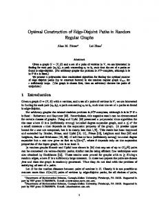
Qj

Qi

Figure 2: Intersection of Qi and Qj .

We may assume that the instance satisfies the conditions (R1) and (R2) by simple reductions. Recall that the k-edge-disjoint paths problem in a graph of tree-width w can be solved in (wO(kw) )nO(1) time by dynamic programming. Thus if the tree-width of G is O(k) and k = O((log n)1/2−ε ) for some ε > 0, then the k-edge-disjoint paths problem in G is solvable in polynomial time of n. With this observation, in order to prove Theorem 6.1, it suffices to show that if the tree-width of G is more than 54k, then the reduction in Section 3.3 happens. Suppose that the tree-width of G is more than 54k. Then, we can take a wall W of height 9k in G by Theorem 6.2. Note that W can be found in polynomial time of n, because t = 9k = O((log n)1/2−ε ) for some ε > 0. Since G is 4-edge-connected, by considering the By Lemma 5.1, L(W ) contains a wall satisfying the case of h = 0, Lemma 5.1 can be modified as follows: conditions in Theorem 5.1. Then, we can find a K3k ′ minor in L(G). The above procedures can be done in Claim 6.1. Let W be a wall of height 2. Then, ′ O(f (k,h)) O(1) comp(W ) contains two edge-disjoint paths connecting (f (k, h) )n time, and if k and h are fixed, the diagonally opposite corners of W ′ . then it can be done in O(m) time. This completes the proof of Theorem 4.1. Let P be the horizonal path in W separating the

Proof. Let Wi′ be the subwall of Wi contained in Wi − per(Wi ) whose size is h. Assume that every vertex in comp(Wi′ ) has degree at most three. Then, in comp(Wi′ ), two paths are edge-disjoint if and only if they are vertex-disjoint. Since Wi′ is flat, by the condition (R2) and the characterization of the feasibility of the two vertex-disjoint paths problem in [34], comp(Wi′ ) can be embedded in a plane so that its infinite face is bounded by per(Wi′ ), which contradicts (C). Hence, comp(Wi′ ) contains a vertex of degree more than three. Then, by the condition (R2) and the characterization of the feasibility of the two edge-disjoint paths problem in [34], comp(Wi ) contains two edge-disjoint paths connecting the diagonally opposite corners of Wi .

i

6 Applications to other cases 6.1 Planar graphs Let us begin with the planar case. For planar graphs, we can improve the “hidden” constant in Theorem 4.2. Namely: Theorem 6.1. Suppose that the input planar graph G is 4-edge-connected or Eulerian, which has n vertices. If k = O((log n)1/2−ε ) for some ε > 0, then the k-edgedisjoint paths problem in G is solvable in polynomial time of n. For the proof, we only use the following theorem instead of Theorem 2.4. Theorem 6.2. ([32], and [29] for an algorithm) Let t be a positive integer. If a planar graph G has tree-width more than 6t, then it contains a wall of height t. Furthermore, such a wall can be found in 2 (tO(t ) )nO(1) time.

351

i-th level of W and the (i + 1)-st level of W for each i. Similarly, let Pi′ be the vertical path in W separating the i-th column of W and the (i + 1)-st column of W for ′ for i = 0, 1, . . . , 3k − 1. each i. Let Qi = P3i+1 ∪ P3i+1 We claim that each Qi can be modified so that the corresponding vertex sets in L(G) form a clique minor of size 3k. We first observe that the intersection of Qi and Qj consists of two paths, and each of them is the “center” of a subwall W ′ of height 2 (Figure 2). Then we can always make a “cross” in L(comp(W ′ )) by Claim 6.1. More precisely, let Q′i , Q′j be the subpaths of Qi , Qj , respectively, in W ′ . Then by Claim 6.1, the paths Q′i , Q′j can be modified in comp(W ′ ) so that they are edgedisjoint and their endpoints are still same. In addition, by the planarity of G, they share a common vertex. We now perform the above operation for each intersection of Qi and Qj for i ̸= j. Then clearly we can modify Qi in comp(W ) so that each Qi is edge-disjoint

Copyright © by SIAM. Unauthorized reproduction of this article is prohibited.

from any other Qj , and any pair Qi and Qj share a common vertex. Thus after contracting all vertices in L(G) corresponding to the edges of the modified Qi , we get a clique minor of order 3k in L(comp(W )). In this case, we can apply the reduction in Section 3.3, which completes the proof. 6.2 Bounded genus graphs and H-minor-free graphs Similarly, we can prove the bounded genus case as well. Theorem 6.3. Suppose that the input graph G can be embedded into a surface with Euler genus g, and is 4edge-connected or Eulerian with n vertices. For any ε > 0, if k = O(min{(log n)1/2−ε , (log(n/g 3/2 ))1−ε }), then the k-edge-disjoint paths problem in G is solvable in polynomial time of n. The proof is almost identical to the planar case. To prove Theorem 6.3, we need the following result obtained by the results in [6, 37]. Suppose G can be embedded into a surface of Euler genus g, and has no flat wall of height t. Then G has tree-width at most O(tg 3/2 ).

did. We just need either a simple reduction as in (A) of Theorem 4.1 or the standard dynamic programming when (B) happens. Suppose (C) happens. Step 2. As proved in (3.1) in [31], if (C) happens, it is possible to throw away a vertex in the deep inside the wall W if h is large enough. This deletion does not change the solution of the problem. Then we just need to recurse our algorithm. For the proof of the correctness for Step 2, we only need the result described in Theorem (3.1) of [31]. Furthermore, it is not so hard to reduce the theorem to the main result in [30]. In fact, if you look at (6) in the proof of Theorem (3.1) in [31], Robertson and Seymour reduce it to the main result in [30]. Thus we can claim that the significant part of Graph Minors XXII [31] is not necessary, and we only need the argument in [30]. Technically, this means that the flat structure of a given wall with bounded number of apex vertices is still troublesome. If we find a disk and an embedded graph in it with a large flat wall, then the proof of the correctness for the algorithm is much easier. References

We can now follow the planar case if we get a flat wall. Then we can prove Theorem 6.3. Similarly, we can prove the H-minor-free case as well. Theorem 6.4. Suppose that the input graph G is 4edge-connected H-minor-free or Eulerian H-minor-free, with n vertices, for fixed graph H. For some ε > 0, 1 if k = O((log log n) 2 −ε ), then the k-edge-disjoint paths problem in G is solvable in polynomial time of n. In order to prove Theorem 6.4, we need the following [7]: There exists a function f such that for an integer t, a fixed graph H, and a H-minorfree graph G, there is a tree-decomposition of G of width w ≤ tf (|V (H)|) or a wall of height t in G. If we use this result instead of Theorem 2.4, the proof of Theorem 4.2 leads to Theorem 6.4. 6.3 General graphs Finally, we describe our algorithm for the edge-disjoint path problem more precisely. Algorithm for the edge-disjoint paths problem Step 1. We first apply Theorem 4.1. If (A) or (B) in Theorem 4.1 happens, it is easy to deal with, as we

352

[1] M. Andrews, J. Chuzhoy, S. Khanna and L. Zhang, Hardness of the undirected edge-disjoint paths problem with congestion, Proc. 46th IEEE Symposium on Foundations of Computer Science (FOCS), 2005, 226– 244. [2] S. Arnborg and A. Proskurowski, Linear time algorithms for NP-hard problems restricted to partial ktrees, Discrete Appl. Math. 23 (1989), 11–24. [3] H. L. Bodlaender, A linear-time algorithm for finding tree-decomposition of small treewidth, SIAM J. Comput. 25 (1996), 1305–1317. [4] C. Chekuri, S. Khanna and B. Shepherd, Edge-disjoint paths in planar graphs, Proc. 45th IEEE Symposium on Foundations of Computer Science (FOCS), 2004, 71–80. [5] C. Chekuri, S. Khanna and B. Shepherd, Edge-disjoint paths in planar graphs with constant congestion, Proc. 38th ACM Symposium on Theory of Computing (STOC), 2006, 757–766. [6] E.D. Demaine and M. Hajiaghayi, Fast algorithms for hard graph problems: Bidimensionality, minors, and local treewidth, Proc. 12th Internat. Symp. on Graph Drawing, Lecture Notes in Computer Science 3383, Springer, 2004, pp. 517–533. [7] E.D. Demaine and M. Hajiaghayi, Linearity of grid minors in treewidth with applications through bidimensionality, Combinatorica 28 (2008), 19–36. [8] R. Diestel, K.Y. Gorbunov, T.R. Jensen and C. Thomassen, Highly connected sets and the excluded grid theorem, J. Combin. Theory Ser. B 75 (1999), 61–73.

Copyright © by SIAM. Unauthorized reproduction of this article is prohibited.

[9] A. Frank, Packing paths, cuts and circuits – a survey, in Paths, Flows and VLSI-Layout, B. Korte, L. Lov´ asz, H.J. Promel and A. Schrijver (Eds.), Springer-Verlag, Berlin, 1990, 49–100. [10] V. Guruswami, S. Khanne, R. Rajaraman, B. Shephard, and M. Yannakakis, Near-optimal hardness results and approximaiton algorithms for edge-disjoint paths and related problems, J. Comp. Styst. Sciences 67 (2003), 473–496. [11] R. Halin, S-functions for graphs, J. Geometry 8 (1976), 171–176. [12] D. Johnson, The many faces of polynomial time, in The NP-completeness column: An ongoing guide, J. Algorithms 8 (1987), 285–303. [13] R.M. Karp, On the computational complexity of combinatorial problems, Networks 5 (1975), 45–68. [14] K. Kawarabayashi, Y. Kobayashi, and B. Reed, The disjoint paths problem in quadratic time, manuscript. [15] J. Kleinberg, An approximation algorithm for the disjoint paths problem in even-degree planar graphs, Proc. 46th IEEE Symposium on Foundations of Computer Science (FOCS), 2005, 627–636. [16] J. Kleinberg and E. Tardos, Disjoint paths in densely embedded graphs, Proc. 36th IEEE Symposium on Foundations of Computer Science (FOCS), 1995, 52– 61. [17] J. Kleinberg and E. Tardos, Approximations for the disjoint paths problem in high-diameter planar networks, Proc. 27th ACM Symposium on Theory of Computing (STOC), 1995, 26–35. [18] M.R. Kramer and J. van Leeuwen, The complexity of wire-routing and finding minimum area layouts for arbitrary VLSI circuits, Adv. Comput. Res. 2 (1984), 129–146. [19] M. Middendorf and F. Pfeiffer, On the complexity of the disjoint paths problem, Combinatorica 13 (1993), 97–107. [20] H. Nagamochi and T. Ibaraki, A linear-time algorithm for finding a sparse k-connected spanning subgraph of a k-connected graph, Algorithmica 7 (1992), 583–596. [21] T. Nishizeki, J. Vygen, and X. Zhou, The edgedisjoint paths problem is NP-complete for seriesparallel graphs, Discrete Appl. Math. 115 (2001), 177– 186. [22] H. Okamura and P.D. Seymour, Multicommodity flows in planar graphs. J. Combin. Theory Ser. B 31 (1981), 75–81. [23] L. Perkovic and B. Reed, An improved algorithm for finding tree decompositions of small width, International Journal on the Foundations of Computing Science 11 (2000), 81–85. [24] B. Reed, Finding approximate separators and computing tree width quickly, Proc. 24th ACM Symposium on Theory of Computing (STOC), 1992, 221–228. [25] B. Reed, Tree width and tangles: a new connectivity measure and some applications, in Surveys in Combinatorics, London Math. Soc. Lecture Note Ser. 241, Cambridge Univ. Press, Cambridge, 1997, 87–162.

353

[26] N. Robertson and P.D. Seymour, Graph minors. II. Algorithmic aspects of tree-width, J. Algorithms 7 (1986), 309–322. [27] N. Robertson and P.D. Seymour, Graph minors. V. Excluding a planar graph, J. Combin. Theory Ser. B 41 (1986), 92–114. [28] N. Robertson and P.D. Seymour, An outline of a disjoint paths algorithm, in Paths, Flows, and VLSILayout, B. Korte, L. Lov´ asz, H.J. Pr¨ omel, and A. Schrijver (Eds.), Springer-Verlag, Berlin, 1990, 267–292. [29] N. Robertson and P.D. Seymour, Graph minors. XIII. The disjoint paths problem, J. Combin. Theory Ser. B 63 (1995), 65–110. [30] N. Robertson and P.D. Seymour, Graph minors. XXI. Graphs with unique linkages, J. Combin. Theory Ser. B 99 (2009), 583–616. [31] N. Robertson and P.D. Seymour, Graph minors. XXII. Irrelevant vertices in linkage problems, manuscript. [32] N. Robertson, P.D. Seymour and R. Thomas, Quickly excluding a planar graph, J. Combin. Theory Ser. B 62 (1994), 323–348. [33] A. Schrijver, Combinatorial Optimization: Polyhedra and Efficiency, Springer-Verlag, 2003. [34] P.D. Seymour, Disjoint paths in graphs, Discrete Math. 29 (1980), 293–309. [35] P.D. Seymour, On odd cuts and plane multicommodity flows, Proceedings of the London Mathematical Society 42 (1981), 178–192. [36] C. Thomassen, 2-linked graph, European Journal of Combinatorics 1 (1980), 371–378. [37] C. Thomassen, A simpler proof of the excluded minor theorem for higher surfaces, J. Combin. Theory Ser. B 70 (1997), 306–311.

Copyright © by SIAM. Unauthorized reproduction of this article is prohibited.