The Efficient Computation of PositionSpecific Match Scores with the Fast Fourier Transform
S. Rajasekaran1, X. Jin1, and J.L. Spouge2*
* Corresponding Author 1
Department of Computer and Information Science and Engineering, University of Florida, Gainesville FL 32611
2
National Center for Biotechnology Information, National Library of Medicine, Bethesda MD 20894
Phone: (301) 435-5912 Fax: (301) 435-2433 Email:
[email protected] For submission to the Journal of Computational Biology Running Title: PSSM Scores and the FFT Version Date: January 9, 2003
Rajasekaran, Xi, and Spouge
PSSM Scores and the FFT
Abstract Historically, in computational biology the fast Fourier transform (FFT) has been used almost exclusively to count the number of exact letter matches between two biosequences. This paper presents an FFT algorithm that can compute the match score of a sequence against a position-specific scoring matrix (PSSM). Our algorithm finds the PSSM score simultaneously over all offsets of the PSSM with the sequence, although like all previous FFT algorithms, it still disallows gaps. Although our algorithm is presented in the context of global matching, it can be adapted to local matching without gaps. As a benchmark, our PSSM-modified FFT algorithm computed pairwise match scores. In timing experiments, our most efficient FFT implementation for pairwise scoring appeared to be 10 to 26 faster than a traditional FFT implementation, with only a factor of 2 in the acceleration attributable to a previously known compression scheme. Many important algorithms for detecting biosequence similarities, e.g., gapped BLAST or PSIBLAST, have a heuristic screening phase that disallows gaps. This paper demonstrates that FFT algorithms merit reconsideration in these screening applications.
Page 1
PSSM Scores and the FFT
Page 2
1. INTRODUCTION The fast Fourier transform (FFT) is an astonishingly efficient algorithm, e.g., (Press et al., 1976). Accordingly, computational biologists have considered its use in at least two separate contexts. First, the Fourier transform detects periodicities within biosequences (Tavare and Giddings, 1989). In protein sequence analysis, e.g., it detects periodicities in profiles of amino acid hydrophobicity (Kubota et al., 1981; McLachlan and Karn, 1983; Cornette et al., 1987) and electron-ion potentials (Veljkovic et al., 1985). Similarly, it detects compositional regularities in DNA sequences (Trifunov and Sussman, 1980; Silverman and Linsker, 1986; Chechetkin and Turygin, 1995; Korotkov et al., 1997). Second, it detects similarities between pairs of biosequences (Felsenstein et al., 1981; Liquori et al., 1986; Benson, 1990; Cheever et al., 1991). The detection of sequence similarity has become central to modern molecular biology. For example, the function of a newly sequenced gene is inferred when the corresponding protein sequence is similar to other, better known proteins in a sequence database (Needleman and Wunsch, 1970; Altschul et al., 1997). It is therefore surprising, perhaps, that despite its astonishing efficiency, the FFT is rarely used for detecting biosequence similarity. This apparent anomaly has a brief explanation. Historically, in computational biology the FFT has been used almost exclusively to count the number of exact letter matches between two biosequences, when the sequences are aligned in an arbitrary offset with gaps disallowed, e.g., (Gusfield, 1999). (See Figure 1.) This usage may reflect computational biologists’ early interest in edit distance, the minimum number of deletions, insertions, or letter substitutions that transform one sequence into another (Ukkonen, 1985). Page 2
PSSM Scores and the FFT
Page 3
Figure 1 near here
On the other hand, experience has shown that for maximum sensitivity, similarity searches in protein databases need to consider chemical and evolutionary relationships between pairs of amino acids (Feng et al., 1984; Altschul et al., 1994). Thus, protein searches use pairwise scoring matrices rather than exact matches to quantify similarity (Altschul, 1991; Altschul, 1993). Scoring matrices also improve the sensitivity of nucleotide similarity searches (States et al., 1991). Sensitivity also improves when gaps are allowed in sequence alignments (Altschul et al., 1997; Altschul, 1999). Accordingly, because similarity searches using exact matches and disallowing gaps are known to be relatively insensitive, the FFT has become discredited as a useful tool for detecting biosequence similarities. When scrutinized, however, the discredit has not been closely justified. In support of this statement, we present an FFT algorithm that can incorporate arbitrary scoring matrices for detecting pairwise similarity between biosequences. Although extant FFT algorithms can be modified to this end, they either make undesirable approximations (Liquori et al., 1986; Cheever et al., 1991) or are extremely inefficient by comparison (Felsenstein et al., 1981; Gusfield, 1999) (see the Results). More importantly for current areas of interest, however, our FFT algorithm can match a protein sequence against the position-specific scoring matrix (PSSM) profiling a protein family (Gribskov et al., 1987; Gribskov et al., 1990; Krogh et al., 1994; Barrett et al., 1997; Karplus et al., 1998). PSSM applications constitute an unexplored possibility for the FFT in computational biology.
Page 3
PSSM Scores and the FFT
Page 4
Throughout this paper, the sequence similarities we describe involve global matches (alignments involving the entire length of two biosequences), as opposed to local matches (alignments of pairs of arbitrary subsequences). FFTs have a reputation of being restricted to global matching, although the reputation is again unmerited. The FFT can be adapted to local matching (Cheever et al., 1991; Rajasekaran et al., 2000). Unfortunately, like all extant FFT algorithms, ours disallows gaps in its sequence alignments. On the other hand, many important algorithms for detecting biosequence similarities, e.g., gapped BLAST or PSIBLAST (Altschul et al., 1997; Altschul and Koonin, 1998; Altschul, 1999) have a heuristic screening phase that likewise disallows gaps when searching for sequence similarity. This paper demonstrates that FFT algorithms merit reconsideration in these screening applications. The remainder of the Introduction gives an abbreviated formal description of the FFT in the context of the exact matching problems that it addressed historically. Thus grounded, our Methods then describe our PSSM modification to the FFT algorithm. The PSSM modification handles pairwise similarity matrices as a special case. The Results then use timing tests to compare our PSSM-modified FFT algorithm to other FFT variants, and a Discussion follows. Our Appendix contains some unimplemented FFT algorithms, including a potentially useful integer compression scheme. We now briefly describe the FFT (Press et al., 1976, p. 304). Consider x = ( x0 , x1 ,..., xn−1 ) and y = ( y0 , y1 ,..., yn−1 ) , two vectors of n complex numbers. The
cyclic cross-correlation of
x
and
y
is defined to be the complex vector
z cyc = ( z0 , z1 ,..., zn−1 ) , where z j = ∑ k =0 x j + k yk and the subscript j + k in the summation is n −1
taken modulo n (Gusfield, 1999). Less formally, set up a circular alignment of the Page 4
PSSM Scores and the FFT
Page 5
vectors x and y , i.e., place xk directly over yk in consecutive evenly spaced positions clockwise around a circle ( k = 0,1,..., n − 1 ). We can compute z j , if we hold x in place
and rotate y
j positions clockwise, multiply the aligned coordinates
(x
j+k
, yk )
( k = 0,1,..., n − 1 ), and then sum the resulting products. Some analogy with biosequence alignments is already apparent. Given x and y , we can compute the cyclic correlation z cyc efficiently with the FFT. If ω = exp ( 2π i / n ) denotes the n th root of unity, the FFT of the complex vector x = ( x0 , x1 , ..., xn−1 )
is
the
X j = x0 + x1ω j + ... + xn−1ω
j ( n −1)
vector
X = ( X 0 , X 1 ,..., X n−1 )
whose
coordinates
are
( j = 0,1,..., n − 1 ). (Following custom, we denote the FFT
of a vector with the corresponding capital letter.) Let y R = ( yn−1 , yn−2 ,..., y0 ) be the reverse of y = ( y0 , y1 ,..., yn−1 ) , and let x : y = ( x0 y0 , x1 y1 ,..., xn−1 yn−1 ) denote the product of x and y coordinate by coordinate. It is well known, e.g., (Horowitz et al., 1998; Gusfield, 1999) that the FFT of z cyc satisfies the equation Z cyc = X : YR , where YR denotes the FFT of y R (not the reverse of the transform Y ). In summary, to find the cyclic cross-correlation z cyc , we reverse y , find the FFTs X and YR of x and y R , take the product Z cyc = X : YR of X and YR coordinate by coordinate, and then perform an FFT inversion. Although there are other mathematical transforms for detecting sequence periodicity, e.g., the Walsh transform (Tavare and Giddings, 1989), the FFT seems unique in its relation to cyclic cross-correlations. Because linear alignments are more common than circular alignments in computational biology, linear cross-correlation is of greater interest to us than its circular Page 5
PSSM Scores and the FFT
Page 6
cousin. Given two vectors x = ( x0 , x1 ,..., xl −1 ) and y = ( y0 , y1 ,..., ym−1 ) , possibly of different lengths, pad x on the left with m − 1 0’s and y on the right with l − 1 0’s to form two vectors x′ = ( 0,0,..., 0, x0 , x1 ,..., xl −1 ) and y′ = ( y0 , y1 ,..., ym−1 ,0,0, ...,0 ) of length n = l + m − 1 . The (linear) cross-correlation z = ( z0 , z1 ,..., zn−1 ) is the cyclic cross-
correlation z′cyc of x′ and y′ . Less formally, set up a linear alignment of the vectors x and y , i.e., place x on a line and y underneath it, with x0 directly over ym−1 and the coordinates evenly spaced. We can compute z j , if we hold x in place and move y j positions to the right, multiply the aligned coordinates from x and y , and then sum the resulting products. Because the computation of the cross-correlation z apparently requires O ( n 2 ) operations, the next fact is somewhat astonishing on first encounter. The FFT and FFT inversions above can be computed in O ( n log n ) time. The divide-and-conquer strategy that accomplishes this magic is standard textbook material, e.g., (Press et al., 1976; Horowitz et al., 1998; Gusfield, 1999). An FFT algorithm for computing the crosscorrelation z therefore only requires O ( n log n ) time. The FFT therefore has been of some interest in biosequence analysis, because it solves the match-count problem for letter strings efficiently (Gusfield, 1999). Consider two sequences A = A0 A1... Al −1 and B = B0 B1...Bm−1 drawn from an alphabet Λ with L letters, and select two (possibly equal) letters a and b from Λ . For each (linear) alignment between two sequences A and B , compute a match count for ( a, b ) , i.e., count the number of times the letter pair ( a, b ) occurs in the alignment. Here, we set up a Page 6
PSSM Scores and the FFT
Page 7
(linear) alignment of the sequences A and B , with A on a line and B underneath, starting with A0 directly over Bm−1 and the letters evenly spaced. Hold A in place and move B to the right
j positions (this position is “the
j th alignment,” for
j = 0,1,..., n − 1 ). Count the number of times z j that the letter pair ( a, b ) occurs in the alignment. The vector z ab = ( z0 , z1 ,..., zn −1 ) gives the match counts. Our notation intentionally suggests that the match count is a special type of crosscorrelation. Let x a be an indicator vector of length l , with 1’s wherever the letter a appears in the sequence A . Let y b be the corresponding indicator vector for the letter b appears in the sequence B . The cross-correlation z ab of x a and y b gives the match counts for ( a, b ) . In Figure 1, e.g., consider match count of the letter pair ( a, t ) for the DNA sequences A = aatcag ( l = 6 ) and B = tctgt ( m = 5 ). The relevant indicator vectors are
x a = (1,1, 0, 0,1, 0 )
and
y t = (1, 0,1, 0,1) , and their cross-correlation
z at = (1,1,1,1, 2,1,1, 0,1, 0 ) gives the match count of ( a, t ) in A and B .
Usually, the total match count z total = ∑ a∈Λ z aa is of primary interest, e.g., for DNA sequences z total = z aa + z cc + z gg + z tt . In Figure 1, e.g., the total match count is z total = ( 0, 0,1, 0,1, 0,3, 0, 0, 0 ) . As shown above, a transformed match count like Z aa can
be computed with two FFTs. Thus, for a general alphabet of L letters, the computation of the total match count appears to require 2L FFTs. Because FFT inversion is a linear operation, however, only a single FFT inversion is required to compute z total = ∑ a∈Λ z aa from the transformed sum Ztotal = ∑ a∈Λ Z aa .
Page 7
PSSM Scores and the FFT
Page 8
A clever encoding scheme reduces the FFT operations required for computing match counts for several letter pairs (Cheever et al., 1991). Instead using a separate indicator vector for each letter, the scheme indicates the positions of two letters in a single vector, indicating the letters with i = −1 as well as 1. In our example from Figure 1, where A = aatcag and B = tctgt , let x at = (1,1, i, 0,1, 0 ) indicate the positions of the letters a
and t in sequence A , and similarly, x cg = ( 0, 0, 0,1, 0,i ) . The indicator vectors for sequence B are similar, except that −i replaces i , so y at = ( −i, 0, −i, 0, −i ) and y cg = ( 0,1, 0, −i, 0 ) . The total match count z total is the real part of z at + z cg , where z at
( z cg ) is the cross-correlation of x at and y at ( xcg and y cg ). The total match count z total can therefore be obtained in L = 4 FFTs and one FFT inversion. If certain approximations are acceptable, the number of FFTs can be reduced even further (Cheever et al., 1991). For reasons given above, however, modern similarity searches rarely count exact matches. Rather, they use scores to indicate different degrees of mismatching. Let S ( a, b ) be the element of an L × L scoring matrix that quantifies the similarity of the
letters a and b . For DNA sequences, e.g., the current BLAST program defaults to scoring
an
exact
nucleotide
S ( a, a ) = ... = S ( t , t ) = 1
and
match
as
1
and
a
mismatch
as
S ( a, c ) = S ( a, g ) = ... = S ( t , g ) = −3
–3,
i.e., (see
http://www.ncbi.nlm.nih.gov/blast/html/blastcgihelp.html#other_advanced). For proteins, the customary PAM or BLOSUM matrices reflect evolutionary relationships by assigning closely related amino acid pairs a positive score (Dayhoff et al., 1978; Henikoff and Henikoff, 1993). The pairwise match score z pair = ( z0 , z1 ,..., zn−1 ) for sequences A and B Page 8
PSSM Scores and the FFT
Page 9
is then of interest, where z j is the sum of the scores of all letter pairs in the j th alignment. The pairwise match score provides a convenient benchmark for our FFT algorithms. Note the equation z pair = ∑ a∈Λ ∑ b∈Λ S ( a, b ) z ab , where z ab is the match count of the letter pair ( a, b ) in A and B . “Algorithm 0,” our benchmark FFT algorithm from the literature (Benson, 1990), calculates z pair from this equation: compute the match counts z ab with the FFT, and then compute their S ( a, b ) -weighted sum. Its time is dominated
by the L2 FFTs required to compute z ab for each letter pair
( a, b )
(because the
transformed sum Z pair = ∑ a∈Λ ∑ b∈Λ S ( a, b ) Z ab only requires one FFT inversion). Thus, Algorithm 0 requires O ( L2 n log n ) time. In our context, the pairwise match score z pair can be considered a specialized position-specific match score, which we define as follows. Let A = A0 A1... Al −1 be a sequence, drawn as usual from our alphabet Λ of L letters. Let S0 , S1 ,..., S m−1 be a sequence of scoring functions, so that Sk assigns a score S k ( a ) to each letter a ∈ Λ . Now, view the values S k ( a ) ( a ∈ Λ ) as the k th column of a position-specific scoring matrix (PSSM) S = ( S0 , S1 , ..., S m−1 ) . The position-specific match score z = ( z0 , z1 ,..., zn−1 ) for the sequence A and the PSSM S can be derived just like the match count or score for two sequences A and B . (See Figure 1.) With S = ( S0 , S1 , ..., S m−1 ) as a formal sequence of column vectors, construct the j th linear alignment of A and S as described above.
Page 9
PSSM Scores and the FFT
Page 10
The j th position-specific match score is the sum of S k ′ ( Ak ) over all aligned pairs
( Ak , Sk′ ) . More formally, let n = l + m − 1 as usual. With the coordinate index j running from 0 to n − 1 ,
z j = ∑ k Sk ′ ( Ak ) ,
(1)
where within the sum, the difference k ′ − k is fixed at m − 1 − j , and the remaining, free index k runs from max {0, j − ( m − 1)} to min {l − 1, j} . For brevity, later equations do not mention the indices and their ranges. They are always the same. Note that the PSSM score contains all historical uses of the FFT as special cases. Let I be the pairwise scoring matrix for exact matching, so I ( a, b ) = 1 if a = b , and I ( a,b ) = 0 otherwise. Note that the matrix I is symmetric: I ( a, b ) = I ( b, a ) . Match
counts
are
the
specialized
PSSM
S k ( a ) = I ( a, Bk )
( k = 0,1,..., m − 1 ),
where
B = B0 B1...Bm−1 is the second match sequence. More generally, pairwise match scores are
the specialized PSSM S k ( a ) = S ( a, Bk ) . Eq (1) therefore provides a formal definition for match counts and pairwise match scores. With this preamble, the Methods now give our PSSM-modified FFT algorithms. When applied to pairwise scoring, they compute z pair in O ( Ln log n ) time, a factor of L faster than the previous O ( L2 n log n ) algorithms.
Page 10
PSSM Scores and the FFT
Page 11
2. METHODS 2.1. Description of the Algorithms Algorithm 1 is as follows. Fix a ∈ Λ . Let x a = ( I ( a, A0 ) , I ( a, A1 ) ,..., I ( a, Al −1 ) ) be the
indicator
vector
of
the
letter
a
in
the
sequence
A,
and
let
y a = S a = ( S0 ( a ) , S1 ( a ) ,..., S m−1 ( a ) ) be the corresponding row of the PSSM S . The
cross-correlation z a = ( za 0 , za1 ,..., za ,n−1 ) of x a and y a equals the position-specific match score attributable to the letter a . The j th coordinate of the position-specific match score attributable to the letter a is zaj = ∑ k I ( a, Ak ) Sk ′ ( a ) . Reversal of summation order gives
∑
a∈Λ
(2)
zaj = ∑ a∈Λ ∑ k I ( a, Ak ) S k ′ ( a ) = ∑ k Sk ′ ( Ak ) = z j
in Eq (1). Thus, the position-specific match score z = ∑ a∈Λ z a . Algorithm 1 can be implemented with the FFT as described in the Introduction. For each a ∈ Λ , the transform Z a of z a can be computed with one FFT. One FFT inversion is required to recover the position-specific match score z from Z = ∑ a∈Λ Z a . Thus, the computational time is O ( Ln log n ) , as advertised. Algorithm 2 is a variant of Algorithm 1, using the compression scheme of Cheever et al. (Cheever et al., 1991) that indicates the positions of two letters with a single vector (hence Algorithm “two”). The Appendix gives a variant compression scheme, Algorithm 2.1.
Page 11
PSSM Scores and the FFT
Page 12
Fix two different letters a, b ∈ Λ . In this encoding, the indicator vector x ab for the letters a and b in sequence A has the coordinates xab , j = I ( a, Aj ) + iI ( b, Aj ) , and with S a and Sb defined as for Algorithm 1, y ab = S a − iSb . The cross-correlation
z ab = ( zab ,0 , zab,1 , ..., zab ,n−1 ) of x ab and y ab has coordinates zab , j = ∑ k { I ( a, Ak ) S k ′ ( a ) + I ( b, Ak ) S k ′ ( b )}
− i ∑ k { I ( a, Ak ) S k ′ ( b ) − I ( b, Ak ) S k ′ ( a )}
.
(3)
Comparison with Eq (2) shows that the real part of z ab equals z a + z b from Algorithm 1. Again, the computational time is O ( Ln log n ) .
2.2. Implementation of the Algorithms We now give our implementations of Algorithms 0, 1, and 2, which we call Implementations 0, 1, and 2. Note that Implementation 0 was a traditional approach (Benson, 1990), which computes one FFT for every letter pair. We describe our implementations for the protein alphabet ( L = 20 letters), although they clearly generalize. Throughout the discourse, we therefore consider two protein sequences
A = A0 A1... Al −1 and B = B0 B1...Bm−1 . Implementation 0 was an implementation of Algorithm 0, which computes a match score for each amino acid pair
( a, b ) .
For each
( a, b ) ,
we took two linear arrays
x = ( x0 , x1 ,..., xn−2 ) and y = ( y0 , y1 ,..., yn−2 ) ( n = l + m − 1 ). The array x indicated the
appearance of a in A , whereas the array y indicated the appearance of b in B . Both x and y were initialized with 0’s. For each k from 0 to l − 1 , the number xm−1+k was set to 1 if Ak = a . Similarly, for each k from 0 to m − 1 , the number yk was set to 1 if Bk = b . Page 12
PSSM Scores and the FFT
Page 13
The array x was therefore padded with 0’s on the left like x′ in the Introduction; y , on the right like y′ . Next, as described in the Introduction, we computed the cyclic cross-correlation of x and y with a textbook C++ program for the FFT (Horowitz et al., 1997). The resulting match count was stored in an array z . All elements in the array z were then multiplied by the similarity score S ( a, b ) , so z now contained the contribution to the match score of A and B from the amino acid pair ( a, b ) . This computation was repeated for every pair ( a, b ) of amino acids, with the overall match score accumulating in a separate array.
Implementation 1 was an implementation of Algorithm 1. We took two linear arrays x and y of length L ( n − 1) each. The array x contained n − 1 structures x k , indexed by k from 0 to n − 2 . Each structure x k was a linear array of L = 20 numbers, indexed from 1 to L = 20 . The entire array x was initialized with 0’s. As in Implementation 0, the structure x m−1+k corresponded to the letter Ak ( k = 0,..., l − 1 ). The exact correspondence was established as follows. First, we imposed an arbitrary order on the L = 20 amino acids. The alphabetical order
ACDEFGHIKLMNPQRSTVWY of the standard single-letter codes was convenient. Accordingly, alanine (A) was the first amino acid, cysteine (C) was the second amino acid, etc. Then, if Ak was the j th amino acid, we set the j th element of the x m−1+k to 1. If sequence A began with DGA, e.g., the three structures x m−1+k ( k = 0,1, 2 ) were Page 13
PSSM Scores and the FFT
Page 14
ACDEFGHIKLMNPQRSTVWY 00100000000000000000 ACDEFGHIKLMNPQRSTVWY 00000100000000000000
ACDEFGHIKLMNPQRSTVWY 10000000000000000000 where the structures appear on separate lines underneath the alphabetical order. The array y also contained n − 1 structures y k , indexed by k from 0 to n − 2 . Each structure y k contained the following L = 20 elements: S k ( A ) , S k ( C ) , S k ( D ) ,..., S k (Y ) , the scores of amino acids A , C , D ,…,Y (alanine, cysteine, glutamate,…, tyrosine) when matched against the amino acid Bk . The cyclic cross-correlation of x and y is the match score. Note that in this implementation of Algorithm 1, only one product in L = 20 from the cross-correlation actually contributes to the match score. Algorithm 1 has a natural implementation with the theoretical time O ( Ln log n ) , slightly better than the theoretical time of O { Ln log ( Ln )} for Implementation 1. Implementation 1 was for us more convenient, however.
Implementation 2 is similar to Implementation 1 except that we used complex indicators to reduce the lengths of x and y . We took two linear arrays x and y of length 1
2
L ( n − 1) each. The array x contained n − 1 structures x k , indexed by k from 0 to
n − 2 . Each structure x k was a linear array of 1
2
1
2
L = 10 numbers, indexed from 1 to
L = 10 . The entire array x was initialized with 0’s. As in Implementation 0, the
Page 14
PSSM Scores and the FFT
Page 15
structure x m−1+k corresponded to the letter Ak ( k = 0,..., l − 1 ). The exact correspondence was established as follows. First, we paired the amino acids in alphabetical order. The following shows the first letter of each pair above the second.
ADFHKMPRTW CEGILNQSVY On one hand, if Ak was the ( 2 j − 1) th amino acid, then we set the j th element of the
x m−1+k to 1. On one hand, if Ak was the ( 2 j ) th amino acid, then we set the j th element of the x m−1+k to i . If sequence A began with DAG, e.g., then the three structures x m−1+k ( k = 0,1, 2 ) were
ADFHKMPRTW
ADFHKMPRTW
0100000000
00i0000000
ADFHKMPRTW 1000000000
CEGILNQSVY
CEGILNQSVY
CEGILNQSVY
where the structures (separated by spaces here) appear between the alternate halves of the alphabetical order. The array y also contained n − 1 structures y k , indexed by k from 0 to n − 2 . The structure
yk
contained
the
following
1
2
L = 10
elements:
S k ( A ) − iS k ( C ) , S k ( D ) − iS k ( E ) ,..., S k (W ) − iS k (Y ) . The real part of the cyclic cross-
correlation of x and y is the match score. Note again that only one product in
1
2
L = 10
from the cross-correlation actually contributes to the match score. Like Implementation 1, Implementation 2 has time O { Ln log ( Ln )} and is convenient but slower than the theoretical time O ( Ln log n ) for Algorithm 2. Page 15
PSSM Scores and the FFT
Page 16
3.
RESULTS
We timed Implementations 0, 1, and 2 with randomly generated sequences as well as sequences downloaded from various NIH databases. This section gives the timing results.
3.1. Simulated Protein Sequences
Figure 2 near here
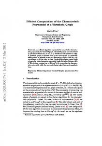
Figure 2 gives our timing of the three Implementations with simulated protein sequences. Our FFT implementation always pads its array sizes up to an integer power of 2. Without the padding, the arrays x and y needed in Implementation 0 are of size n − 1 ; in Implementation 1, of size L ( n − 1) ; and in Implementation 2, of size
1
2
L ( n − 1) . Here,
L = 20 and n = l + m − 1 is one less than twice the sequence length.
Implementation 0 therefore uses FFT array sizes of 64 for sequences of lengths 25 and 32. Implementation 1 uses array sizes of 1024 for sequences of length 25, doubling to 2048 for sequences of length 32. Implementation 2 always requires half the array size of Implementation 1. When sequence lengths were scaled up by factors of 8, 16, 32, and 64 (i.e., powers of 2), the required array sizes scaled accordingly. The corresponding choices of sequence lengths (shown in Figure 2) permit a comparison of Implementation 0 and 1 under conditions that favor first one implementation and then the other. Figure 2 can be summarized as follows. Implementation 1 is between about 5 to 12 times faster Implementation 0, depending on whether the sequence lengths favor it or not. Implementation 2 is about twice as fast as Implementation 1. All comparisons between the implementations are consistent, regardless of the scale of sequence length. Page 16
PSSM Scores and the FFT
Page 17
3.2. Real Protein Sequences We downloaded six proteins from http://www.ncbi.nlm.nih.gov. Their accession numbers, followed in parentheses by their sequence lengths, were AAD14597.1 (440), CAA56071.1 (445), BAA34431.1 (622), AAB65242.1 (670), AAB60937.1 (1224), and BAA13219.1 (1496). We selected these protein sequences because they form three pairs of similar sizes: (440,445), (622,670), and (1224,1496). Figure 3 gives our timing of the three Implementations with these real protein sequences.
Figure 3 near here
Figure 3 can be summarized as follows. Implementation 1 is about 12 times faster than Implementation 0. Implementation 2 is about 26 times faster than Implementation 0. All comparisons between the implementations are consistent, regardless of the sequence lengths.
Page 17
PSSM Scores and the FFT
Page 18
4. DISCUSSION In this paper, we modified the FFT for the efficient computation of PSSM scores. Our PSSM-modified FFT algorithm computes PSSM scores simultaneously over all alignment offsets between a sequence and a PSSM. Within the context of our algorithm, match counts and pairwise scoring are merely special PSSMs. Traditional FFT algorithms cannot handle PSSMs. Thus, we needed to use traditional FFT algorithms with pairwise scoring as benchmarks for our PSSM-modified FFT algorithm. Our FFT algorithm for pairwise scoring appeared to be 5 to 12 times faster than the traditional algorithm (compare Implementation 0 and Implementation 1 in the Results). A previously known compression scheme (Cheever et al., 1991) made our FFT algorithm twice as fast as before: other improvements to our implementations are also readily available. For example, the Appendix gives Algorithm 3, a compression scheme. In addition, although the Introduction describes the FFT operation within the complex number field, the FFT can also be performed within the field of integers modulo a prime number. We did not explore the efficiencies of integer arithmetic, but it sometimes speeds FFT computations considerably (Benson, 1990). Because specialized, ultra-fast hardware is also available for digital signal processing, our PSSM-modified FFT algorithm has considerable potential for further acceleration. Although our PSSM-modified FFT algorithm was presented in the context of global matches, FFT algorithms can be adapted to local matching (Cheever et al., 1991; Rajasekaran et al., 2000). Thus, the disallowance of gaps in FFT matching remains the main obstacle to wide application in bioinformatics. On the other hand, many important algorithms for detecting biosequence similarities, e.g., gapped BLAST or PSIBLAST Page 18
PSSM Scores and the FFT
Page 19
(Altschul et al., 1997; Altschul and Koonin, 1998; Altschul, 1999), have a heuristic screening phase that also disallows gaps. The FFT might find uses in such applications.
Page 19
PSSM Scores and the FFT
Page 20
APPENDIX Algorithm 2.1 is one of many possible variants of Algorithm 2. Define the vectors x ab and S a just as in Algorithm 2, but now define y ab = S ab =
1
2
(1 + i ) S a + 1 2 (1 − i ) Sb . The
cross-correlation z ab = ( zab ,0 , zab ,1 ,..., zab ,n−1 ) of x ab and y ab has coordinates zab , j =
The
1
2
real
(1 + i ) ∑ k {I ( a, Ak ) Sk ′ ( a ) + I ( b, Ak ) Sk ′ ( b )} . + 1 2 (1 − i ) ∑ k { I ( a, Ak ) Sk ′ ( b ) − I ( b, Ak ) S k ′ ( a )} and
imaginary
∑ {I ( a, A ) S ( a ) + I ( b, A ) S ( b )} = z k
k
k′
k
k′
parts aj
of
zab , j
sum
(4)
to
+ zbj from Eq (2).
Our point here is that indicators can be encoded into complex vectors in many ways. Algorithm 2 is simpler than (and therefore preferable to) Algorithm 2.1, however.
Algorithm 3 is a variant of Algorithm 1 that applies to PSSMs S with integer entries S k ( a ) ( a ∈ Λ and k = 0,1,..., m − 1 ). Algorithm 3 might be especially useful when the
FFT is performed within the field of integers modulo a prime number (Benson, 1990). In a search for local similarity (Cheever et al., 1991), n = l + m − 1 might be particularly small. For convenience and without loss of generality, we replace the L letters a ∈ Λ by the numbers a = 0,1,..., L − 1 . Algorithm 3 is a compression scheme modulo R , where the integer radix R bounds the
range
of
the
cross-correlations
zaj
in
Eq
(2),
i.e.,
0 ≤ ∑ k max a Sk ′ ( a ) − ∑ k min a Sk ′ ( a ) < R . Such bounds are easily estimated. Subtract the constant ck = min a S k ( a ) from each column in S to form a matrix S′ , i.e., S k′ ( a ) = S k ( a ) − ck for a = 0,1,..., L − 1 . The elements of the matrix S′ are all zeros or Page 20
PSSM Scores and the FFT
Page 21
counting numbers, because min a S k′ ( a ) = min a S k ( a ) − ck = 0 . The matrix S′ also satisfies 0 = ∑ k min a S k′′ ( a ) ≤ ∑ k max a Sk′′ ( a ) < R . Define vectors x
and y
xk = ∑ a=0 I ( a, Ak )R L−1−a L −1
with integer coordinates
( k = 0,1, ..., l − 1 ) and yk = ∑ a=0 S k′ ( a )R a ( k = 0,1,..., m − 1 ). Define also the vector L −1
y c = ( c0 , c1 ,..., cm−1 ) . Then the cross-correlation of x and y is z = ( z0 , z1 ,..., zn−1 ) , where
the integer
L−1 L−1 L−1 z j = ∑ ∑ I ( a, Ak ) R L−1−a ∑ Sk′′ ( a ) R a = ∑ ∑ Sk′′ ( a ) R L−1+a− Ak . k a =0 a =0 a =0 k
(5)
Because 0 ≤ ∑ k Sk′′ ( a ) < R for all k ′ and all a = 0,1,..., L − 1 , the L th digit of z j in base R (i.e., the term a = Ak from the right side of Eq (5)) is
∑
k
Sk′′ ( Ak ) . Let z ( L ) be the
vector of L th digits from z j in base R , and let z c be the cross-correlation of (1,1, ...,1) and y c . The coordinates of the vector z ( L ) + z c are the desired PSSM scores
∑
k
S k ′ ( Ak ) = ∑ k {S k′′ ( Ak ) + ck′ } .
The time required for Algorithm 3 is the sum of O ( Lm ) for the computation of S′ and O ( n log n ) for the FFTs, as long as the denser encoding does not increase the time for computing the integer additions and multiplications.
Page 21
PSSM Scores and the FFT
Page 22
REFERENCES Altschul, S. 1999. Hot papers - Bioinformatics - Gapped BLAST and PSI-BLAST: a new generation of protein database search programs by S.F. Altschul, T.L. Madden, A.A. Schaffer, J.H. Zhang, Z. Zhang, W. Miller, D.J. Lipman - Comments. Scientist. 13, 15-15. Altschul, S.F. 1991. Amino acid substitution matrices from an information theoretic perspective. J Mol Biol. 219, 555-65. Altschul, S.F. 1993. A protein alignment scoring system sensitive at all evolutionary distances. J Mol Evol. 36, 290-300. Altschul, S.F., Boguski, M.S., Gish, W. and Wootton, J.C. 1994. Issues in searching molecular sequence databases. Nat Genet. 6, 119-29. Altschul, S.F. and Koonin, E.V. 1998. Iterated profile searches with PSI-BLAST--a tool for discovery in protein databases. Trends Biochem Sci. 23, 444-7. Altschul, S.F., Madden, T.L., Schaffer, A.A., Zhang, J., Zhang, Z., Miller, W. and Lipman, D.J. 1997. Gapped BLAST and PSI-BLAST: a new generation of protein database search programs. Nucleic Acids Res. 25, 3389-402. Barrett, C., Hughey, R. and Karplus, K. 1997. Scoring hidden Markov models. Comput Appl Biosci. 13, 191-9. Benson, D.C. 1990. Fourier methods for biosequence analysis. Nucleic Acids Res. 18, 6305-10. Chechetkin, V.R. and Turygin, A.Y. 1995. Search of Hidden Periodicities in DNASequences. Journal of Theoretical Biology. 175, 477-494.
Page 22
PSSM Scores and the FFT
Page 23
Cheever, E.A., Overton, G.C. and Searls, D.B. 1991. Fast Fourier transform-based correlation of DNA sequences using complex plane encoding. Comput Appl Biosci. 7, 143-54. Cornette, J.L., Cease, K.B., Margalit, H., Spouge, J.L., Berzofsky, J.A. and Delisi, C. 1987. Hydrophobicity Scales and Computational Techniques For Detecting Amphipathic Structures in Proteins. Journal of Molecular Biology. 195, 659-685. Dayhoff, M.O., Schwartz, R.M. and Orcutt, B.C. 1978. A model of evolutionary change in proteins, 345-352. eds., Atlas of Protein Sequence and Structure, National Biomedical Research Foundation, Silver Spring, MD. Supp 3. Felsenstein, J.S., Sawyer, S. and Kochin, R. 1981. An efficient method for matching nucleic acid sequences. Nucleic Acids Research. 10, 133-139. Feng, D.F., Johnson, M.S. and Doolittle, R.F. 1984. Aligning amino acid sequences: comparison of commonly used methods. J Mol Evol. 21, 112-25. Gribskov, M., Luthy, R. and Eisenberg, D. 1990. Profile analysis. Methods Enzymol. 183, 146-59. Gribskov, M., McLachlan, A.D. and Eisenberg, D. 1987. Profile analysis: detection of distantly related proteins. Proc Natl Acad Sci U S A. 84, 4355-8. Gusfield, D. 1999. Algorithms on Strings, Trees, and Sequences. Cambridge University Press, Cambridge. Henikoff, S. and Henikoff, J.G. 1993. Performance evaluation of amino acid substitution matrices. Proteins. 17, 49-61. Horowitz, E., Sahni, S. and Rajasekaran, S. 1997. Computer Algorithms/C++. W. H. Freeman Press, New York.
Page 23
PSSM Scores and the FFT
Page 24
Horowitz, E., Sahni, S. and Rajasekaran, S. 1998. Computer Algorithms. W. H. Freeman Press, New York. Karplus, K., Barrett, C. and Hughey, R. 1998. Hidden Markov models for detecting remote protein homologies. Bioinformatics. 14, 846-56. Korotkov, E.V., Korotkova, M.A. and Tulko, J.S. 1997. Latent sequence periodicity of some oncogenes and DNA-binding protein genes. Computer Applications in the Biosciences. 13, 37-44. Krogh, A., Brown, M., Mian, I.S., Sjolander, K. and Haussler, D. 1994. Hidden Markov models in computational biology. Applications to protein modeling. J Mol Biol. 235, 1501-31. Kubota, Y., Takahashi, S., Nishikawa, K. and Ooi, T. 1981. Homology in protein sequencs expressed by correlation coefficients. Journal of Theoretical Biology. 91, 347-361. Liquori, A.M., Ripamonti, A., Sadun, C., Ottani, S. and Braga, D. 1986. Pattern recognition of sequence similarities in globular proteins by Fourier analysis: a novel approach to molecular evolution. J Mol Evol. 23, 80-7. McLachlan, A.D. and Karn, J. 1983. Periodic features in the amino acid sequence of nematode myosin rod. J Mol Biol. 164, 605-26. Needleman, S.B. and Wunsch, C.D. 1970. A general method applicable to the search for similarities in the amino acid sequence of two proteins. Journal of Molecular Biology. 48, 443-453. Press, W.H., Teukolsky, S.A., Vetterling, W.T. and Flannery, B.P. 1976. Numerical Recipes in C. Cambridge University Press, Cambridge.
Page 24
PSSM Scores and the FFT
Page 25
Rajasekaran, S., Nick, H., Pardalos, P.M., Sahni, S. and G., S. 2000. Efficient Algorithms for Local Alignment Search. Journal of Combinatorial Optimization. To appear. Silverman, B.D. and Linsker, R. 1986. A measure of DNA periodicity. Journal of Theoretical Biology. 118, 295-300. States, D.J., Gish, W. and Altschul, S.F. 1991. Improved sensitivity of nucleic acid database searches using application-specific scoring matrices. Methods. 3, 66-70. Tavare, S. and Giddings, B. 1989. Some statistical aspects of the primary structure of nucleotide sequences, 117-132. In M. S. Waterman, eds., Mathematical Methods for DNA Sequences, CRC Press, Boca Raton, FL. Trifunov, E.N. and Sussman, J.L. 1980. The pitch of chromatin DNA is reflected in its nucleotide sequence. Proceedings of the National Academy of Sciences. 77, 38163820. Ukkonen, E. 1985. Algorithms for approximate string matching. Information and Control. 64, 100-118. Veljkovic, V., Cosic, I., Dimitrijevic, B. and Lalovic, D. 1985. Is it possible to analyze DNA and protein sequences by the methods of digital signal processing? IEEE Trans Biomed Eng. 32, 337-41.
Page 25
Rajasekaran, Xi, and Spouge
A
Figure 1
a a t c a g
B S
t c t g t a c g t
-4 -4 -4 5
Page 26
-4 5 -4 -4
-4 -4 -4 5
-4 -4 5 -4
-4 -4 -4 5
Rajasekaran, Xi, and Spouge
Legend for Figure 1
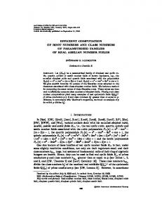
Figure 4. A gapless global alignment between two sequences A = aatcag and B = tctgt . In the alignment shown, B is offset 2 to the right from A . The alignment shown has a total match count of 3 from the exact match A = aatcag and B = tctgt . The edit distance between A and B is 4, with the corresponding edit operations as follows. Delete the initial two a ’s in A , delete the final t in B , and substitute g for the third a in A . For pairwise scoring, the BLAST default for DNA sequences gives a score 5 to an exact letter match and –4 to a mismatch. The global alignment shown matches four letters for a pairwise match score of 5+5-4+5=11. The figure also shows a PSSM S , which corresponds to the BLAST default for pairwise scoring when a sequence is aligned with
B . Thus, the alignment shown between A and S has a PSSM score of 5+5-4+5=11, which equals the pairwise score (as indeed it must). If the final three letters tgt in B (and these alone) are shifted one position to the right, an alignment allowing gaps is generated. If we consider only the subsequences cag in A and ctg in B , and ignore the relationships and scores for any other letters, a local alignment is generated. This paper considers only global alignments disallowing gaps: local alignments or alignments allowing gaps are not explicitly considered.
Page 27
Rajasekaran, Xi, and Spouge
Figure 2
time (seconds)
100 10 1 0.1 256
512
1024
2048
sequence lengths (letters)
Figure 5. A timing comparison of the three Implementations with simulated protein sequences. Sequence lengths are shown on the X-axis; the corresponding timing results, on the logarithmic Y-axis. All times shown are the averages over ten random pairs. For each of the sequence lengths 256, 512, 1024, and 2048, ten pairs of random sequences were generated. The corresponding times are given by the black bars for Implementation 0, the diagonally striped bars for Implementation 1, and by the white bars for Implementation 2. For reasons given in the text, ten pairs of random sequences were also generated for each of the sequence lengths 200, 400, 800, and 1600. The corresponding times for Implementation 1 are given by the vertically striped bars.
Page 28
Rajasekaran, Xi, and Spouge
Figure 3
time (seconds)
100 10 1 0.1 (440,445)
(622,670)
(1224,1496)
sequence lengths (letters) Figure 6. A timing comparison of the three Implementations with real protein sequences. The pairs of sequence lengths are shown on the X-axis; the corresponding timing results, on the logarithmic Y-axis. The corresponding times are given by the black bars for Implementation 0, the diagonally striped bars for Implementation 1, and by the white bars for Implementation 2.
Page 29