The finite volume element method in nonconvex polygonal domains P. Chatzipantelidis — R.D. Lazarov Department of Mathematics, Texas A&M University, College Station, TX, 77843, USA, e-mails: [email protected], [email protected] We consider standard finite volume piecewise linear approximations for second order elliptic boundary value problems on a nonconvex polygonal domain. Based on sharp shift estimates, we derive error estimations in H 1 – and L2 –norm, taking into consideration the regularity of the data. ABSTRACT.

KEYWORDS:

Finite volume element method, nonconvex polygons, error estimations

1. Introduction In this note we study the convergence of the standard finite volume element method for discretization of second order linear elliptic pde’s on a non-convex polygonal domain Ω ⊂ R2 with Dirichlet boundary conditions. Namely, for a given function f , we seek u such that Lu = f,

in Ω,

and

u=0

on ∂Ω,

(1.1)

2

with Lv ≡ − div(A∇v), A = A(x) = (aij )i,j=1 a given symmetric matrix function with real–valued entries aij ∈ W 1,∞ , 1 ≤ i, j ≤ 2. We assume that the matrix A(x) is uniformly positive definite in Ω, i.e., there exists a positive constant α0 such that ξ T A(x)ξ ≥ α0 ξ T ξ,

¯ ∀ξ ∈ R2 , ∀x ∈ Ω.

(1.2)

Finite volume discretizations for more general convection–diffusion–reaction problems were studied by many authors (for a comprehensive presentation and more references of existing results we refer to [EGH–00]). For convex polygonal domains, H 1 and L2 norm error estimates were derived in [EWI–02], taking into account the regularity of f . Our goal in this paper is to study the influence of the corner singularities and insufficient regularity of the right–hand side f , say f ∈ Lp (Ω), p < 2,

2

Finite volumes for complex applications

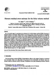
Ω ω0

S0

Figure 1. A non-convex domain Ω with a corner S0 and ω0 > π.

or f ∈ H −` (Ω), 0 ≤ ` < 1/2, on the convergence rate of the finite volume element method. We note that we use the conservative version of the method, namely the right–hand side of the scheme is computed by the L2 –inner product of f with the characteristic functions of the finite volumes (or equivalently by the duality between H ` and H −` for 0 ≤ ` < 1/2). For more singular f , i.e. f ∈ H −` , 0 ≤ ` ≤ 1, we refer to [DRO–02]. Our analysis of the error estimates in H 1 and L2 norm follows the approach developed in [CHA–02] and uses known sharp regularity results for the solutions of elliptic boundary value problems, cf. [GRI–85].

2. Preliminaries In this paper we use standard notation for Sobolev spaces W s,p and H s = W s,2 , cf. [ADA–75]. Namely, Lp denotes the space of p−integrable real functions over Ω, | · |s and k · ks the seminorm and norm, respectively, in H s = H s (Ω), | · |W s,p and k · kW s,p the seminorm and norm, respectively, in W s,p = W s,p (Ω), p ≥ 1, and s ∈ R. If s = 0 we suppress this index. Let us first consider the Dirichlet problem for Poisson’s equation: Given f ∈ Lp , p ≥ 1, find a function u : Ω → R2 such that −∆u = f,

in Ω,

and

u=0

on ∂Ω,

(2.1)

with Ω a bounded, non-convex, polygonal domain in R. For simplicity we assume that Ω has only one inner angle greater than π, namely ω0 ∈ (π, 2π), cf. Figure 1. It is known that there exists a unique solution u ∈ H01 of (2.1). Furthermore, u could be represented in the form u = c0 w0 + v, where v ∈ W 2,p ∩ H01 , c0 is a constant and w0 = rλm √ω10 λm sin(λm θ)η(reiθ ). Here λm = mπ ω0 , m ∈ N, η is a cutoff function which is one near S0 and zero away from S0 and (r, θ) are the polar coordinates with respect to the vertex S0 with angle ω0 . A crucial role in determining the regularity of u is played by the 2 . constant p0 ≡ 2−π/ω 0

FVM in Nonconvex Polygons

3

If f ∈ Lp , p ≥ 1, in view of [GRI–85, p. 233] and a standard imbedding result, we have that u ∈ H s with s = 2 − s0 − δ(p), where s0 and δ(p) > 0 are defined by ½ 2 2 2 π p < p0 , p − p0 , s0 = −1=1− , δ(p) = (2.2) arbitrarily small, p ≥ p0 . p0 ω0 Further, if f ∈ H −` , 0 ≤ ` ≤ 1 the solution u of (2.1) satisfies u ∈ H s , with s = 2 − s0 − δ(`), where δ(`) > 0 is defined by ½ ` − s0 , s0 < ` ≤ 1, δ(`) = (2.3) arbitrarily small, 0 ≤ ` ≤ s0 . For the more general problem (1.1) similar results hold. Let A and T , 2 be matrices such that A = (aij (S0 ))i,j=1 and −T T AT = I. Also, let ω0 (A) be the measure of the angle at T S0 of T Ω, with T Ω = {T x : x ∈ Ω} and 2 . Then in view of [GRI–85, Theorem 5.2.7], if f ∈ Lp , p ≥ 1, p0 (A) = 2−π/ω 0 (A) the solution u of (1.1) is in H s , with s = 2 − s0 − δ(p), where in the definition of s0 and δ, (2.2), we substitute p0 (A) for p0 . In the rest of this paper, we will denote by s = 2 − s0 − δ, where s0 and δ are defined as above, depending if we are referring to problem (1.1) or (2.1) and whether f is in Lp , p ≥ 1 or H −` , ` ∈ [0, 1]. 3. The finite volume element method We consider a quasi uniform family {Th }0

0 arbitrary small. Also, if in the construction of the control volumes bz , zK is the barycenter of the triangle K then, there exists a constant C, independent of h, such that ¡ ¢ ku − uh k ≤ C h2(s−1) kuks + hs kf k + hmin (2,s+2−2/p) kf kW 1,p = O(h2(s−1) ). Proof: The proof is similar to that of Theorem 4.1. It is obvious that it suffices to estimate the term II in (4.12). Since f ∈ W 1,p , we have f ∈ L2 , and therefore u ∈ H s , with s = 2 − s0 − δ. Due to (4.11) and Lemmas 4.1 and 4.2, we obtain ¡ ¢ |II| ≤ C h2 (|f |W 1,p + |u|s ) + hku − uh k1 |χ|W 1,q , ∀χ ∈ Xh0 , with 1/p + 1/q = 1. Choosing now χ to be an appropriate interpolant of ϕ, with appropriate stability properties, and using standard imbedding arguments and an inverse inequality we obtain ¡ ¢ 2 ku − uh k ≤ C h2(s−1) kuks + hs kf k + hmin (2,s+2−2/p) kf kW 1,p ku − uh k. We can easily see that since 3/2 < s < 2 we have 2(s − 1) ≤ s. Also, the fact that s ≤ 2 ≤ 4 − 2/p suggests 2(s − 1) < min (2, 2 + s − 2/p). Combining now these with the above error estimation we obtain the desired result. ¤ Remark 4.3 Our L2 –norm error estimates are in contrast to known estimates for the finite element method. For example, the finite element approximation

8

Finite volumes for complex applications

Table 1. Convergence rate for exact solution u = (r2/3 + rβ )sin(2θ/3) β H 1 -norm L2 -norm

1/2 0.54 (0.50) 1.20 (1.00)

2/3 0.66 (0.66) 1.34 (1.34)

3/4 0.69 (0.66) 1.37 (1.34)

4/5 0.69 (0.66) 1.37 (1.34)

FE 0 uFE h , defined by a(uh , χ) = (f, χ), ∀χ ∈ Xh , is known to satisfy, cf., e.g., [BRE–94, Chapter 12], s−1 ku − uFE kuks , h k1 ≤ Ch

2(s−1) ku − uFE kuks . h k ≤ Ch

In Table 4 we present the computed rates of convergence of the finite volume method which illustrate the results of Theorem 4.1. We considered the Dirichlet boundary value problem for the Poisson equations in an L-shaped domain with an exact solution u = (r2/3 +rβ )sin(2θ/3). One can see that u is almost in H 3/2 if β = 1/2 and u is almost in H 5/3 if β ≥ 2/3. The numerical experiments show that the finite volume scheme recovers the solution with the expected rates in H 1 -norm. The convergence rates in L2 -norm in some cases are slightly higher than the ones predicted by the theory. References [ADA–75] Adams, R.A., Sobolev Spaces, Academic Press, New York, 1975. [BAN–87] Bank, R.E. and Rose, D.J., “Some error estimates for the box method”, SIAM J. Numer. Anal., vol. 24, 1987, pp. 777–787. [BRE–94] Brenner, S.C. and Scott, L.R., The Mathematical Theory of Finite Element Methods, Springer–Verlag, New York, 1994. [CHA–02] Chatzipantelidis, P., “Finite volume methods for elliptic partial differential equations: A new approach”. To appear in M2AN. ¨t, T., “Finite volume discretization [DRO–02] Droniou, J. and Galloue of noncoercive elliptic equations with general right–hand sides”. (in this proceedings). ¨t, T. and Herbin, R., Finite Volume [EGH–00] Eymard, R., Galloue Methods, Handbook of Numerical Analysis, Vol. VII, pp. 713-1020, North Holland, Amsterdam, 2000. [EWI–02] Ewing, R.E., Lin, T. and Lin, Y., “On the accuracy of the finite volume element method based on piecewise linear polynomials”, SIAM J. Numer. Anal., vol. 39, 2002, pp. 1865–1888. [GRI–85] Grisvard, P., Elliptic Problems in Nonsmooth Domains, Pitman, Massachusetts, 1985.