The Fixed-Mesh ALE approach for the numerical ... - UPCommons

The Fixed-Mesh ALE approach for the numerical approximation of flows in moving domains Ramon Codina1,∗ , Guillaume Houzeaux2 , Herbert Coppola-Owen1 and Joan Baiges1 International Center for Numerical Methods in Engineering (CIMNE), Universitat Polit`ecnica de Catalunya, Jordi Girona 1-3, Edifici C1, 08034 Barcelona, Spain. Barcelona Supercomputing Center, Jordi Girona 29, Edifici Nexus II, 08034 Barcelona, Spain. ∗ [email protected] 1

2

Contents 1 Introduction

2

2 The Fixed-Mesh ALE method 2.1 The classical ALE method and its finite element approximation 2.1.1 Problem statement . . . . . . . . . . . . . . . . . . . . 2.1.2 The time-discrete problem . . . . . . . . . . . . . . . 2.1.3 The fully discrete problem . . . . . . . . . . . . . . . 2.2 The fixed-mesh ALE approach: algorithmic steps . . . . . . . . 2.3 Other fixed grid methods . . . . . . . . . . . . . . . . . . . .

. . . . . .

. . . . . .

. . . . . .

. . . . . .

. . . . . .

. . . . . .

. . . . . .

. . . . . .

. . . . . .

. . . . . .

. . . . . .

. . . . . .

. . . . . .

. . . . . .

. . . . . .

. . . . . .

. . . . . .

. . . . . .

. . . . . .

. . . . . .

3 3 3 4 5 7 8

3 Developing the Fixed-Mesh ALE method 3.1 Step 1. Boundary function update . . . . . . . . . . . . . . . . . . . . . 3.2 Step 2. Mesh velocity . . . . . . . . . . . . . . . . . . . . . . . . . . . 3.3 Step 3. Solving the flow equations I: Equations on the deformed mesh . . 3.4 Step 4. Splitting of elements . . . . . . . . . . . . . . . . . . . . . . . . 3.5 Step 5. Solving the flow equations II: Equations on the background mesh 3.6 Comparison with the classical ALE approach . . . . . . . . . . . . . . .

. . . . . .

. . . . . .

. . . . . .

. . . . . .

. . . . . .

. . . . . .

. . . . . .

. . . . . .

. . . . . .

. . . . . .

. . . . . .

. . . . . .

. . . . . .

. . . . . .

. . . . . .

. . . . . .

. . . . . .

. . . . . .

. . . . . .

10 10 10 11 11 12 12

4 Side numerical ingredients 4.1 Level set function update . . . . . . . . . . . . . . . . . . . . . . . . . . . . . . . . . . . . . . . . . . . . 4.2 Approximate imposition of boundary conditions . . . . . . . . . . . . . . . . . . . . . . . . . . . . . . . . 4.3 Data transfer between finite element meshes . . . . . . . . . . . . . . . . . . . . . . . . . . . . . . . . . .

13 13 14 16

5 A numerical example

17

6 Two applications 6.1 Lost foam casting . . . . . . . . . . . . . . . . . . . . . . . . . . . . . . . . . . . . . . . . . . . . . . . . 6.2 Free surface flows . . . . . . . . . . . . . . . . . . . . . . . . . . . . . . . . . . . . . . . . . . . . . . . .

21 21 23

7 Conclusions

25

1

. . . . . .

. . . . . .

. . . . . .

. . . . . .

Abstract In this paper we propose a method to approximate flow problems in moving domains using always a given grid for the spatial discretization, and therefore the formulation to be presented falls within the category of fixed-grid methods. Even though the imposition of boundary conditions is a key ingredient that is very often used to classify the fixed-grid method, our approach can be applied together with any technique to impose approximately boundary conditions, although we also describe the one we actually favor. Our main concern is to properly account for the advection of information as the domain boundary evolves. To achieve this, we use an arbitrary LagrangianEulerian framework, the distinctive feature being that at each time step results are projected onto a fixed, background mesh, that is where the problem is actually solved.

1 Introduction In many coupled problems of practical interest the domain of at least one of the problems evolves in time. The Arbitrary Eulerian Lagrangian (ALE) approach is a tool very often employed to cope with this domain motion. In this work we aim at describing a particular version of the ALE formulation that can be used in different coupled problems, and which we will apply to two problems in fluid mechanics. In the classical ALE approach to solve problems in computational fluid dynamics, the mesh in which the computational domain is discretized is deformed (see for example [13, 29, 27]). This is done according to a prescribed motion of part of its boundary, which is transmitted to the interior nodes in a way as smooth as possible so as to avoid mesh distortion. In this work we present an ALE-type strategy with a different motivation. Instead of assuming that the computational domain is defined by the mesh boundary, we assume that there is a function that defines the boundary of the domain where the flow takes place. We will refer to it as the boundary function. It may be given, for example, by the shape of a body that moves within the fluid, or it may need to be computed, as in the case of level set functions described in the paper. It may be also defined discretely, by a set of points. When this boundary function moves, the flow domain changes, and that must be taken into account at the moment of writing the conservation equations that govern the flow, which need to be cast in the ALE format. However, our purpose here is to explain how to use always a background fixed mesh. That requires a virtual motion of the mesh nodes followed by a projection of the new node positions onto the fixed mesh. The basic numerical formulation we will use consists of a stabilized finite element method to solve the ALE flow equations and finite difference time integration schemes. However, other discretization techniques could be applied, since the idea we want to expose is independent of the numerical method being used. This idea consists in projecting the results of the ALE deformed mesh onto a fixed background mesh at each time step, prior to solving the flow equations. It will be shown that at the end all the calculations can be performed on the fixed mesh, and in fact the ALE deformed mesh does not need to be explicitly built. We want to stress that this idea is independent on the way to impose boundary conditions on the moving boundary. The way to impose this prescription is often used to classify a particular fixed-mesh method. Since the physical boundary is contained in the domain actually discretized, these methods are often called immersed boundary methods. Moreover, since the fixed grid used is often Cartesian, these formulations can be found under the keywords Cartesian grid methods (see for example the reviews [42, 36, 35]). These methods are developed for constant-in-time domains, and then extended in a more or less ad-hoc way to time dependent domains. In spite of the fact that we want to distinguish between the way to deal with moving domains from the way of approximately imposing the boundary conditions on the moving boundary, we will briefly describe the particular approach we use. The paper is organized as follows. A general overview of the FM-ALE method is presented in 2

Section 2, starting with the discretization of the classical ALE formulation and then describing the algorithmic steps of the FM-ALE alternative. These steps are further elaborated in Section 3. Even though they are not intrinsic to the main idea of the method, there are three numerical ingredients that are essential for the success of the formulation. These are the definition and updating of the moving boundary, the approximate imposition of boundary conditions and the projection of data between two different finite element meshes. These “side ingredients” have been published before [10, 8, 24], but are here particularized to the FM-ALE method. They are described in Section 4. A simple numerical example, but containing all the features of the formulation, is presented in Section 5. We discuss then the application of the FM-ALE idea to two coupled problems of practical interest in Section 6. One is the simulation of lost foam casting [26]. In this case the flow is coupled to the heat equation because of the interface evolution, which is governed by the advance of the burning front of the molten metal used in the casting. Therefore, the boundary velocity is given and the normal stress on the fluid is unknown. The second problem considered is a classical free surface problem in which, once more, the free surface position is modeled by a level set function [12]. In this case, the velocity on the free surface is unknown, but the normal stress can be prescribed to zero (or to the atmospheric pressure). Some conclusions close the paper in Section 7.

2 The Fixed-Mesh ALE method In this section we describe the essential idea of the FM-ALE method. However, we start with the classical ALE formulation of the incompressible Navier-Stokes equations and their numerical approximation.

2.1

The classical ALE method and its finite element approximation

2.1.1 Problem statement Let us consider a region Ω0 ⊂ Rd (d = 2, 3) where a flow will take place during a time interval [0, T ]. However, we consider the case in which the fluid at time t occupies only a subdomain Ω(t) ⊂ Ω 0 (note in particular that Ω(0) ⊂ Ω0 ). Suppose also that the boundary of Ω(t) is defined by part of ∂Ω 0 and a moving boundary that we call Γfree (t) = ∂Ω(t) \ ∂Ω0 ∩ ∂Ω(t). This moving part of ∂Ω(t) may correspond to the boundary of a moving solid immersed in the fluid or can be determined by a level set function, as we will see in the applications. In order to cope with the time-dependency of Ω(t), we use the ALE approach, with the particular feature of considering a variable definition of the domain velocity. Let χ t be a family of invertible mappings, which for all t ∈ [0, T ] map a point X ∈ Ω(0) to a point x = χ t (X) ∈ Ω(t), with χ0 = I, the identity. If χt is given by the motion of the particles, the resulting formulation would be Lagrangian, whereas if χt = I for all t, Ω(t) = Ω(0) and the formulation would be Eulerian. Let now t0 ∈ [0, T ], with t0 ≤ t, and consider the mapping χt,t0 : Ω(t0 ) −→ Ω(t) 0 x0 7→ x = χt ◦ χ−1 t0 (x ).

Given a function f : Ω(t) × (0, T ) −→ R we define ¯ ∂(f ◦ χt,t0 ) 0 ∂f ¯¯ (x , t), (x, t) := ∂t ¯x0 ∂t

x ∈ Ω(t), x0 ∈ Ω(t0 ).

In particular, the domain velocity taking as a reference the coordinates of Ω(t 0 ) is given by ¯ ∂x ¯¯ udom := (x, t). ∂t ¯ 0 x

3

(1)

The incompressible Navier-Stokes formulated in Ω(t), accounting also for the motion of this domain, can be written as follows: find a velocity u : Ω(t) × (0, T ) −→ R d and a pressure p : Ω(t) × (0, T ) −→ R such that ¯ ¸ · ∂u ¯¯ (x, t) + (u − udom ) · ∇u − ∇ · (2µ∇S u) + ∇p = ρf , (2) ρ ∂t ¯x0 ∇ · u = 0,

(3)

where ∇S u is the symmetrical part of the velocity gradient, ρ is the fluid density, µ is the viscosity and f is the vector of body forces. Initial and boundary conditions have to be appended to problem (2)-(3). In the applications we have considered in Section 6, the boundary conditions on Γ free (t) can be of two different types: a) Free surface flows: p (or the normal stress) given, u unknown on Γ free ; b) Lost foam casting: u given, p (or the normal stress) unknown on Γfree . On the rest of the boundary of Ω(t) the usual boundary conditions can be considered. In general, we consider these boundary conditions of the form ¯ on ΓD , u=u n · σ = ¯t on ΓN , ¯ where n is the external normal to the boundary, σ = −pI + 2µ∇ S u is the Cauchy stress tensor and u and ¯t are the given boundary data. The components of the boundary Γ D and ΓN are obviously disjoint and such that ΓD ∪ ΓN = ∂Ω, and therefore time-dependent. 2.1.2 The time-discrete problem Let us start introducing some notation. Consider a uniform partition of [0, T ] into N time intervals of length δt. Let us denote by f n the approximation of a time dependent function f at time level t n = nδt. We will also denote δf n+1 = f n+1 − f n , f n+1 − f n , δt = θf n+1 + (1 − θ)f n ,

δt f n+1 = f n+θ

θ ∈ [1/2, 1].

Even though other options are obviously possible, we will use the simple trapezoidal rule to discretize problem (2)-(3) in time. Suppose we are given a computational domain at time t n , with spatial coordinates labeled xn , and un and pn are known in this domain. The velocity un+1 and the pressure pn+1 can then be found as the solution to the problem h i ¯ n+θ ) · ∇u ρ δt un+1 ¯xn + (un+θ − un+θ − ∇ · (2µ∇S un+θ ) + ∇pn+1 = ρf n+1 , (4) dom ∇ · un+θ = 0,

(5)

¯ where now δt un+1 ¯xn = (un+1 (x) − un (xn ))/δt, being x = χtn+θ ,tn (xn ) the spatial coordinates in Ω(tn+θ ). The domain velocity given by (1), with x0 = xn , is approximated as un+θ dom =

¢ 1 ¡ χtn+θ ,tn (xn ) − xn . θδt

(6)

Note that the order of accuracy of this approximation is consistent with the order of accuracy of (4)-(5), that is to say, it is 2 for θ = 1/2 and 1 otherwise. We are interested only in the cases θ = 1/2 and θ = 1 (implicit schemes are required). 4

Remark 1 The trapezoidal rule considered for the time integration, with a single mesh, satisfies the so called geometric conservation law (GCL) condition. However, there are second order accurate schemes based on multi-step time discretizations that do not satisfy it. The price to be paid is that these schemes are usually only conditionally stable, although stability conditions are often very mild and not encountered in practice (see for example the analyses in [1, 3, 16, 17, 38]). We will use one of such schemes in Section 5. 4 2.1.3 The fully discrete problem The next step is to consider the spatial discretization of problem (4)-(5). As for the time discretization, different options are possible. Here we simply describe the stabilized finite element formulation employed in our numerical simulations. Let {Ωe }n+1 be a finite element partition of the domain Ω(tn+1 ), with index e ranging from 1 to the number of elements nel (which may be different at different time steps). We denote with a subscript h the finite element approximation to the unknown functions, and by v h and qh the velocity and pressure test functions associated to {Ωe }n+1 , respectively. An important point is that we are interested in using equal interpolation for the velocity and the pressure. Therefore, the corresponding finite element spaces are assumed to be built up using the standard continuous interpolation functions. In order to overcome the numerical problems of the standard Galerkin method, a stabilized finite element formulation is applied. This formulation is presented in [6]. It is based on the subgrid scale concept introduced in [28], although when linear elements are used it reduces to the Galerkin/leastsquares method described for example in [18]. We apply this stabilized formulation together with the finite difference approximation in time (4)-(5). The bottom line of the method is to test the continuous equations by the standard Galerkin test functions plus perturbations that depend on the operator representing the differential equation being solved. In our case, this operator corresponds to the linearized form of the time discrete Navier-Stokes equations (4)-(5). In this case, the method consists of finding u n+1 and pn+1 such that h h ¯ ¡ ¢ ¯ n , v h + an+θ (uh , v h ) + cn+θ (uh − udom ; uh , v h ) + bn+θ (ph , v h ) = ln+θ (v h ), mn+θ δt un+1 1 1 1 h x (7) ¯ ¢ ¡ n+θ n+θ n+1 ¯ n+θ n+θ (qh , uh ) + s (qh , ph ) = l (qh ), qh , δ t u m n + b 2

h

x

2

2

(8)

for all test functions v h and qh , the former vanishing on the Dirichlet part of the boundary Γ D . The

5

different forms appearing in these equations are given by Z nel Z X ζ u1 · ρ δt uh , v h · ρ δ t uh + m1 (δt uh , v h ) = e e=1 Ω nel Z X

Ω

a(uh , v h ) =

Z

2∇S v h : µ∇S uh + Ω

Z

c(a; uh , v h ) = b1 (ph , v h ) = −

m2 (qh , δt uh ) =

e=1 nel Z X

v h · (ρ a · ∇uh ) + Ω

Z

e=1

ph ∇ · v h + Ω

b2 (qh , uh ) = s(qh , ph ) =

nel Z X

l1 (v h ) = l2 (qh ) =

e=1

nel Z X e=1

Ωe

Ωe

Ωe

ζu2 ∇ · uh ,

ζ u1 · (ρ a · ∇uh ) ,

ζ u1 · ∇ph ,

Ωe

¡ ¢ ζ p · ρ a · ∇uh − 2∇ · (µ∇S uh ) ,

ζ p · ∇ph ,

vh · f + Ω

nel Z X e=1

Ωe

Ωe

e=1

Z

ζ p · ρ δ t uh ,

Ω

nel Z X

nel Z X

Ωe

qh ∇ · u h +

e=1

Z

nel Z X e=1

e=1

Z

Ωe

nel ¡ ¢ X ζ u1 · −2∇ · (µ∇S uh ) +

Ωe

ζ u1 · f +

Z

v h · ¯t, ΓN

ζp · f ,

where the functions ζ u1 , ζu2 and ζ p are computed within each element as £ ¤ ζ u1 = τu ρ (uh − udom ) · ∇v h + 2∇ · (µ∇S v h ) ,

(9)

ζu2 = τp ∇ · v h ,

(10)

ζ p = τu ∇qh ,

(11)

and the parameters τu and τp are also computed element-wise as (see [7]) · ¸ 4µ 2ρ|uh − udom | −1 τu = , τp = 4µ + 2ρ|uh − udom |h, + h2 h where h is the element size for linear elements and half of it for quadratics. Remark 2 • The superscript n + θ in all the terms in (7)-(8) indicates that all the forms are evaluated with the unknowns at n + θ, except for the term coming from the temporal derivative, whose superscript is explicitly indicated. Likewise, the integrals are evaluated at Ω(t n+θ ). • The dependency on the advection velocity a = uh − udom has been only indicated in the from coming directly from the convective term of the equations, namely, c(a; u h , v h ). However, it has to be noted that all the forms listed above depend on the stabilization parameters, and therefore depend on a as well. Moreover, the dependency of b 2 (qh , uh ) on a is even more explicit. However, in order to keep the notation more concise only the above mentioned dependency of c(a; uh , v h ) has been left. 6

• As usual, the mesh of Ω(tn+1 ) is assumed to be obtained from the mesh of Ω(tn ) by moving the nodes of the latter with the domain velocity udom (often referred to as mesh velocity). This greatly simplifies the implementation of the ALE method, since in this case the nodal values of u n+1 (x) and those of un (xn ) correspond to the same nodes (at time steps n + 1 and n, respectively). ¯ ¯ n= • If θ = 1/2, the unknowns of the problem can be taken as u n+1/2 and pn+1/2 , since δt un+1 h x −1 2δt (un+1/2 (x) − un (xn )). All the calculations to be performed are the same as for θ = 1, with the only modification that once un+1/2 is computed un+1 has to be updated to go to the next time step. This analogy includes the updating of the computational domain. When θ = 1/2 we need to update this domain from n − 1/2 to n + 1/2 to compute u n+1/2 and pn+1/2 , whereas when θ = 1 we need to update it from n to n + 1 to compute u n+1 and pn+1 . For conciseness, the latter situation is considered in the following. • From (9)-(11) it is observed that these terms are precisely the adjoints of the (linearized) operators of the differential equations to be solved applied to the test functions (observe the sign of the viscous term in (9)). This method corresponds to the algebraic version of the subgrid scale approach ([28]) and circumvents the stability problems of the Galerkin method. In particular, in this case it is possible to use equal velocity pressure interpolations, that is, we are not tight to the satisfaction of the inf-sup stability condition. For more details about this formulation, see for example [28, 6]. • In order to simplify a little bit the statement of the problem, we will consider that m 2 (qh , δt uh ) = 0. This can be justified by using a space-time finite element method with constant-in-time interpolation (in the case θ = 1) or by using the orthogonal-subscale stabilization (OSS) method (see [7]). 4

2.2

The fixed-mesh ALE approach: algorithmic steps

The purpose of this subsection is to give an overview of the FM-ALE method and to describe the main idea, leaving for the next section a more detailed description of the different steps involved. Suppose Ω0 is meshed with a finite element mesh M 0 and that at time level tn the domain Ω(tn ) is meshed with a finite element mesh M n (as we will see, close to M 0 ). Let un be the velocity already computed on Ω(tn ). The purpose is to obtain the fluid region Ω(tn+1 ) and the velocity field un+1 . The former may move according to a prescribed kinematics, for example due to the motion of a solid, or can be an unknown of the problem, as in the two applications we will describe in Section 6. If the classical ALE method is used, M n would deform to another mesh defined at tn+1 . The key idea is not to use this mesh to compute un+1 and pn+1 , but to re-mesh in such a way that the new mesh is, essentially, M 0 once again. The steps of the algorithm to achieve the goal described are the following: 1. Define Γn+1 free by updating the function that defines it. n+1 2. Deform virtually the mesh M n to Mvirt using the classical ALE concepts and compute the mesh n+1 velocity um . n+1 3. Write down the ALE Navier-Stokes equations on Mvirt . n+1 ), M n+1 . 4. Split the elements of M 0 cut by Γn+1 free to define a mesh on Ω(t

7

n+1 5. Project the ALE Navier-Stokes equations from Mvirt to M n+1 .

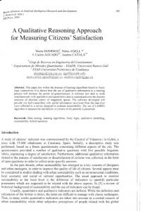
6. Solve the equations on M n+1 to compute un+1 and pn+1 . In Section 3 we describe all these steps in detail. A global idea of the meshes involved in the process is represented in Fig. 1. Note in particular that at each time steps two sets of nodes have to be appropriately dealt with, namely, the so called newly created nodes and the boundary nodes. Contrary to other fixed grid methods, some of which are described in the next subsection, newly created nodes are treated in a completely natural way using the FM-ALE approach: the value of the velocity there is n+1 directly given by the projection step from Mvirt to M n+1 . Boundary nodes require either additional unknowns with respect to those of mesh M 0 or an appropriate imposition of boundary conditions. This issue is treated in Section 4.

Figure 1: Two dimensional FM-ALE schematic. Top-left: original finite element mesh M 0 of Ω0 . Topright: finite element mesh M n of Ω(tn ), with the elements represented by a thick line and the elements of M 0 represented by thin line. The blue line represents Γnfree and the red edges indicate the splitting of n+1 M 0 to obtain M n . Bottom-left: updating of M n to Mvirt using the classical ALE strategy. The position n+1 of Γfree is again shown using a solid blue line and the previous position Γ nfree using a dotted blue line. Bottom-right: Mesh M n+1 of Ω(tn+1 ), represented by a thick line. The edges that split elements of M 0 are again indicated in red. Boundary nodes, where approximate boundary conditions need to be imposed, are drawn in green, whereas newly created nodes are drawn in gray.

2.3

Other fixed grid methods

Other possibilities to use a single grid in the whole simulation can be found in the literature, each one having advantages and drawbacks. As the method presented in this paper, they were designed as an 8

alternative to body fitted meshes and are sometimes referred to as Embedded Mesh Methods. They can be divided into two main groups [9], corresponding in fact to two ways of prescribing the boundary conditions on Γfree : • Force term. The interaction of the fluid and the solid is taken into account through a force term, which appears either in the strong or in the weak form of the flow equations. Therefore, the boundary conditions on Γfree are neither imposed as Dirichlet nor as Neumann boundary conditions. Among this type of methods, let us cite for example the Immersed Boundary method as a variant of the Penalty method, where punctual forces are added to the momentum equation, and the Fictitious Domain method, where the solid boundary conditions are imposed through a Lagrange multiplier. • Approximate boundary conditions. Instead of adding a force term, these methods impose the boundary conditions in an approximate way once the discretization has been carried out, either by modifying the differential operators near the interface (in finite differences) or by modifying the unknowns near the interface. The Immersed Boundary Method in its original form [40] consists in adding punctual penalty forces in the domain boundary so that the boundary conditions are fulfilled. The forces are computed from a fluid-structure (elastic) interaction problem at the interface. The method is first order accurate even if second order approximation schemes are used, although formal second order accuracy has been reported in [32]. The more recent Immersed Interface Method achieves higher order accuracy by avoiding the use of the Dirac delta distribution to define the forcing terms (see [33, 34, 44]). The Penalty method is similar to the previous one in the sense that a force term is added to the momentum equations. The difference raises in the fact that the penalty parameter is not computed from a fluid-structure interaction as in the original immersed boundary method, but it is simply required to be large enough to enforce the boundary conditions approximately. The force terms can be of two types, depending on whether they are imposed as boundary or as volume forces [43] . Another approach is the use of Lagrange multipliers to enforce the boundary conditions. However, the finite element subspaces for the bulk and Lagrange multiplier fields must satisfy the classical infsup condition, which usually leads to the need for stabilization (see [23, 2, 30]). Moreover, additional degrees of freedom must be added to the problem. The use of Lagrange multipliers is the basis of the Fictitious Domain Method [20, 21]. Recently, hybrid Cartesian/immersed boundary methods have been developed for Cartesian grids, which use the grid nodes closest to the boundary to enforce boundary conditions [19, 45, 37]. The method is second order accurate. Most of these methods have been well tested in the literature for both steady and moving interfaces. Generally, the last case is treated by applying directly the former at each time step. However, very few authors have described the full formulation for moving interfaces, sometimes simply by ignoring the problem. The fact that the boundary moves and the subsequent advection of unknowns is often not taken into account. To explain an obvious consequence of the boundary motion, let us discuss the treatment of the newly created nodes. To explain the problem, let us consider point P in Fig. 1. Suppose that the boundary Γ free corresponds in this case to the rigid boundary of a moving object. Physically, it is clear that the solution in the fluid cannot depend on what happens inside the solid. Mathematically, this means that the values of the unknowns at the fluid nodes are uncoupled from those at the solid nodes. Therefore, the velocity and the pressure at the solid nodes (apart from those participating to the enforcing of the boundary conditions) can be whatever at a certain time step n, in particular their value at node P (see Fig. 1, topright). Now we move on to the next time step n + 1 as the solid moves. Some solid nodes can therefore 9

become fluid nodes, such as node P (see Fig. 1, bottom-right). The velocity at this node at time step n is in fact needed in the temporal term of the momentum equations and cannot be whatever. In the case of fractional step techniques, the situation can even be worse as the previous time step pressure could also be needed at these nodes. A special treatment is needed for the newly created fluid nodes. In many publications, the previous time step values are computed using ad hoc arguments, that sometimes lead to good approximations from the practical point of view when small time steps are used. As an example, in [35] the authors extrapolate the velocity and pressure from the nearest fluid nodes at the previous time step. In [5], the Navier-Stokes equations are correctly expressed in an ALE framework, but the velocity is taken as the solid velocity. It is worth to note that if the solid is deformable and has been solved together with the fluid in a coupled way (as in the original immersed boundary method [40] or in the fluid-solid approach in [46]), this velocity is physically meaningful. This is not the case, however, is the case of rigid bodies or bodies with rigid boundaries. A possibility to deal with this situation is to write the Navier-Stokes equations in a non-inertial frame of reference attached to the body, as in [25] in the context of Chimera meshes or in [31], where an immersed boundary method is used. We explain in the following what we believe is a consistent way of treating moving interfaces based on a fixed-mesh ALE approach.

3 Developing the Fixed-Mesh ALE method In this section we describe the steps enumerated previously, concentrating on those specific of the FMALE method and leaving for Section 4 those that can be considered side numerical ingredients.

3.1

Step 1. Boundary function update

This step is completely problem dependent. The motion of Γ free (t) may be determined by different ways. In a typical fluid-structure interaction problem, Γfree (t) will be part of the solid boundary, and therefore its kinematics will be determined by the dynamics of the solid under the action exerted by the fluid. As a particular case, the motion of the solid boundary may be directly prescribed. This is the simplest situation and the one corresponding to the validating numerical example presented in Section 5. In a wide variety of applications, Γfree (t) may be represented by a level set function. In Section 6 we will describe two of these applications. The peculiarities of the level set function update in the context of the FM-ALE approach are described in Section 4.

3.2

Step 2. Mesh velocity

Updating the boundary function defines the deformation of the domain from Ω(t n ) to Ω(tn+1 ) (recall that we are considering the case θ = 1, see Remark 2). Consequently, the mesh M n used at time step n has to be deformed to adapt to the domain Ω(tn+1 ). This mesh deformation has to be defined by means of a mesh velocity. and xnb , where The mesh velocity on the boundary points can be computed from their position x n+1 b subscript b refers to points on Γfree . Using approximation (6), this mesh velocity would be u n+1 dom,b = n+1 n (xb − xb )/δt. Once the velocity at the nodes of Γfree is known, it has to be extended to the rest of the nodes. A classical possibility is to solve the Laplace problem ∆u dom = 0 using un+1 dom,b as Dirichlet boundary conditions. However, it is also possible to restrict u dom 6= 0 to the nodes next to Γn+1 free , since in our approach mesh distortion does not accumulate from one time step to another (see Fig. 1 for a schematic of the mesh deformation). This is in practice what we do. Details about this point are provided in the numerical examples of Sections 5 and 6. 10

3.3

Step 3. Solving the flow equations I: Equations on the deformed mesh

n+1 The previous procedure defines the domain Ω(tn+1 ) and a mesh that we call Mvirt , obtained from a n deformation of the mesh M . The equations to be solved there are (see (7)-(8)): µ ³ ¶ ´ 1 n+1 n+1 n n m1 uh,virt (x) − uh,virt (x ) , v h + an+1 (uh,virt , v h ) δt

+ cn+1 (uh,virt − udom,virt ; uh,virt , v h ) + bn+1 (ph,virt , v h ) = l1n+1 (v h ), 1

bn+1 (qh , uh,virt ) 2

+s

n+1

(qh , ph,virt ) =

l2n+1 (qh ),

(12) (13)

n+1 where subscript “virt” refers to the mesh Mvirt on which these equations should now be solved using the space discretization described in Subsection 2.1.3. Let us stress once again that, as it is well known n+1 in the classical ALE approach, un (xn ) is known on Mvirt because the nodes of this mesh are obtained n from the motion of the nodes of M with the mesh velocity un+1 dom,virt .

3.4

Step 4. Splitting of elements

n+1 The key idea of the FM-ALE method is not to use Mvirt to solve the flow equations at time tn+1 , but n+1 to use instead another mesh M that will be a a minor modification of the background mesh M 0 . n+1 This mesh M is obtained by splitting the elements of M 0 cut by Γn+1 free , as shown in Fig. 1. Meshes n+1 0 M and M only differ in the subelements created after the splitting just mentioned. Mesh M n+1 could be thought as a local refinement of mesh M 0 to make it conform the boundary Γn+1 free . This is certainly a possibility that can be implemented as such. Let us note however that this requires the introduction of boundary nodes at each step, as shown in Fig. 1, and the subsequent change in the mesh graph and in the sparsity pattern of the matrix of the final algebraic system to be solved for the arrays of nodal unknowns. As in other fixed grid methods, this computational complication can be avoided by prescribing boundary conditions on Γn+1 free in an approximate way. Nevertheless, this issue, in spite of its major practical importance, is not an essential concept of the FM-ALE method, and we defer its description to Section 4. The local refinement from M 0 to M n+1 is needed also to perform the numerical integration of the different terms appearing in (7)-(8). Obviously, the impact of this in the computational cost of the overall calculation is minimum. The splitting of elements is a strictly algorithmic step that shall not be discussed here. In the case of 2D linear elements, Fig. 2 shows how the splitting can be done and the numerical integration points (red points) required in each triangle resulting from this splitting.

1

2

3 Figure 2: Splitting of elements

11

3.5

Step 5. Solving the flow equations II: Equations on the background mesh

n+1 Let P n+1 be the projection of finite element functions defined on Mvirt to M n+1 . To define it, for each n+1 node of M n+1 the element in Mvirt where it is placed has to be identified. Once this is done, the value of any unknown at this node can be obtained through interpolation, possibly with restrictions. The way to construct this projection operator is a problem common to different situations in which transfer of information between finite element meshes is required. We describe our approach in Section 4. n+1 The velocity un in Mvirt is known because its nodal values correspond to those of mesh M n . However, its nodal values on M n+1 have to be computed using the projection just described. The same happens with the mesh velocity udom . If now we define

un+1 := P n+1 (un+1 h h,virt ), the problem to be solved at time step n + 1 is to find a velocity u n+1 and a pressure pn+1 such that h h ¡ −1 ¡ n+1 ¢ ¢ δt mn+1 uh (x) − P n+1 (unh,virt (xn )) , v h + an+1 (uh , v h ) 1

(14)

bn+1 (qh , uh ) 2

(15)

+ cn+1 (uh − P n+1 (udom,virt ); uh , v h ) + bn+1 (ph , v h ) = l1n+1 (v h ), 1 +s

n+1

(qh , ph ) =

l2n+1 (qh ),

which again must hold for all velocity test functions v h and pressure test functions qh . n+1 is divergence is determined by imposing that un+1 6= P n+1 (pn+1 Note that pn+1 h h,virt ). Pressure ph h n+1 free, which at the discrete level is not equivalent to impose that u h,virt is divergence free. Problem (14)-(15) is posed on M n+1 which, as it has been said, coincides with M 0 except for the splitting of the elements crossed by the interface. Even this difference can be avoided if instead of prescribing exactly the boundary conditions an approximation is performed, for example using Nitsche’s method, Lagrange multipliers or the strategy described in Section 4. Therefore, the goal of using a fixed mesh during the whole simulation has been achieved. It is observed that the projection P n+1 has to be applied to • P n+1 (unh,virt (xn )). This clarifies the effect of the mesh motion in the context of fixed-mesh methods. In particular, there is no doubt about the velocity at previous time steps of newly created nodes. n+1 • P n+1 (un+1 dom,virt ). The mesh velocity is computed on Mvirt , and therefore needs to be projected to compute on M n+1 .

3.6

Comparison with the classical ALE approach

To conclude this section, it is important to highlight the differences between our FM-ALE approach and a classical ALE formulation: • Given a position of the fluid front on the fixed mesh, elements cut by the front are split into subelements (only for integration purposes), so that the front coincides with the edges of the subelements. • After deforming the mesh from one time step to the other using classical ALE procedures, results are projected back to the original mesh . 12

• The front is represented by a boundary function, and not by the position of the material points at Γfree as in a classical ALE method.

4 Side numerical ingredients In this section we describe some numerical ingredients that, in spite of being essential in the development of the FM-ALE method, are not inherent to its main concept. In other words, these ingredients may be changed without altering the main concept of the method.

4.1

Level set function update

In the applications, there are several ways to define Γfree . In general, we assume that this part of the boundary of the flow domain is defined by what we have called generically a boundary function. This function may be defined analytically or by discrete means, for example through interpolation from some nodes that define the location of Γfree . That would be a natural way to deal with fluid-structure interaction problems. In some applications, as those described in Section 6, it is convenient to represent Γ free by a level set function (see [39] for an overview of these methods). This function, say ψ, will be the solution of the problem in Ω0 × (0, T ),

∂t ψ + u · ∇ψ = 0 ψ=ψ

(16)

on Γinf × (0, T ),

ψ(x, 0) = ψ0 (x)

in Ω0 ,

where Γinf := {x ∈ ∂Ω0 | u · n < 0} is the inflow part of the domain boundary. In free surface simulations, the initial condition ψ0 is chosen in order to define the initial position of the fluid front to be analyzed. The boundary condition ψ determines whether fluid enters or not through a certain point of the inflow boundary. Due to the pure convective type of the equation for ψ, we use the SUPG technique for the spatial discretization. Again, the temporal evolution is treated via the standard trapezoidal rule. If ψ is taken as a step function, numerical problems may be encountered when it is transported. It is known that small oscillations in the vicinity of sharp gradients still remain using the SUPG formulation. These oscillations may propagate and yield to distorted front shapes, specially near corners. Compared to similar methods, such as the volume-of-fluid (VOF) method [22], one particularity of the level set method is that it uses a smooth function ψ. As the smoothness can be lost as the simulation evolves, the level set function must be redefined for each mesh node as explained for example in [10]. Once ψ is computed, Γfree (t) is defined as Γfree (t) = {x ∈ Ω0 | ψ(x, t) = 0}. Thus, Γfree (t) is simply updated by solving the problem for ψ(x, t). The important point to be noted is that the system is solved on the whole domain Ω 0 . As mentioned earlier, we approximate this problem using a stabilized finite element method. For the discrete problem it is necessary to extrapolate the velocity defined on Ω(t) to the rest of Ω 0 . The question is how to perform this extrapolation. In principle, the advection velocity u in (16) is only needed in the neighborhood of Γfree (t), since the precise transport of ψ is not needed, except for the transport of the isovalue that defines Γfree (t). In our calculations, we have found useful to extrapolate u by solving a Stokes problem on Ω(t)c = Ω0 \ Ω(t). This has two main advantages with respect to a simpler extrapolation procedure, namely, the extrapolated velocity is weakly divergence free in Ω(t) c and we can impose the correct boundary conditions for it. 13

4.2

Approximate imposition of boundary conditions

Even though we have not formulated it as such, the FM-ALE method can be considered an immersed boundary method, in the sense that Γfree (t) is a boundary that moves within a fixed domain Ω0 . From the conceptual point of view, there is no problem in imposing exactly Dirichlet boundary conditions on this part of the boundary. However, this requires the dynamic addition of mesh nodes (see Fig. 1, where these nodes are drawn in green), with the associated change in the sparsity of the matrix of the algebraic system to be solved mentioned earlier. This is why it is very convenient from the implementation standpoint to avoid the explicit introduction of such nodes and to prescribe boundary conditions approximately. We summarize next the strategy proposed in [8] to prescribe Dirichlet boundary conditions on a generic immersed boundary, that we denote by Γ. Let uh be the unknown solution of a problem posed in Ω ⊂ Ω0 for which we want to prescribe a condition on Γ. Let ΩΓ be the set of elements cut by Γ, which is split as ΩΓ = ΩΓ,in ∪ ΩΓ,out , where ΩΓ,in = Ω ∩ ΩΓ and ΩΓ,out is the interior of ΩΓ \ ΩΓ,in . Let also Ωin be such that Ω = Ωin ∪ ΩΓ,in . For simplicity, we will assume that the intersection of Γ with the element domains can be exactly represented by the classical isoparametric mapping. For the notation to be used, see Fig. 3 (left). Suppose that the unknown uh is interpolated as uh (x) =

nin X

a a Iin (x)Uin

a=1

+

n out X

b b Iout (x)Uout

b=1

= I in (x)U in + I out (x)U out , a (x) and I b (x) are the standard interpolation functions, n is the number of nodes in Ω , where Iin in in out the domain where the problem needs to be solved (including layer L 0 ) and nout the number of nodes in layer L−1 (see Fig. 3).

Figure 3: Immersed boundary sketch (left) and domain of extrapolation (right) in a 2D example The objective is to compute U out . Suppose that uh needs to be prescribed to a given function u ¯ on

14

Γ. The main idea is to compute U out by minimizing the functional Z Z 2 (I in (x)U in + I out (x)U out − u ¯(x))2 . ¯(x)) = J2 (U in , U out ) = (uh (x) − u

(17)

Γ

Γ

Suppose now that the problem for uh in Ωin leads to an algebraic equation of the form (18)

K in,in U in + K in,out U out = F in .

The domain integrals in matrices K in,in and K in,out extend only over Ω. The nodal values U out are merely used as degrees of freedom to interpolate uh in the domain Ω. If (18) is supplemented with the equation resulting from the minimization of functional (17), the system to be solved is finally ¸ · ¸· ¸ · K in,in K in,out U in F in , (19) = NΓ MΓ U out fΓ where MΓ =

Z

Γ

I tout (x)I out (x),

fΓ =

Z

Γ

I tout (x)¯ u(x),

NΓ =

Z

Γ

I tout (x)I in (x).

It is important to note that this implementation maintains the connectivity of the background mesh. As it is explained in detail in [8], this method works well if the boundary Γ is not too close to layer L0 in Fig. 3 (left). If this is not the case, the idea is to use the nodes of this layer to prescribe the boundary conditions in an approximate way, and to impose the equation to be solved at the rest of nodes of Ωin . Let E be the extrapolation operator of functions defined on the elements in contact with ∂Ω in to ΩΓ,in . The first point to consider is how to choose the extrapolation region of this operator E. There are several possibilities, but the one we have found most accurate is the following. Let K be an element with an edge (in 2D) or face (in 3D) F on ∂Ωin . Let KΓ be the cylinder obtained from projecting F onto Γ in a way orthogonal to Γ. Then, E is defined as the extension from functions defined on K to functions defined on K ∪ KΓ . The extrapolation regions obtained this way in 2D using triangular elements are shown in Fig. 3 (right). Suppose now that in Ωin the unknown uh is interpolated as uh (x) =

n1 X

I1a (x)U1a +

a=1

n00 X

b b I00 (x)U00

b=1

= I 1 (x)U 1 + I 00 (x)U 00 , b (x) are the standard interpolation functions, n is the number of nodes interior to where I1a (x) and I00 1 Ωin (up to layer L1 ) and n00 the number of nodes in layer L0 (see Fig. 3). The objective is to compute U 00 . We propose to obtain it by minimizing the functional Z Z J20 (U 1 , U 00 ) = (Euh (x) − u ¯(x))2 = (EI 1 (x)U 1 + EI 00 (x)U 00 − u ¯(x))2 , Γ

Γ

which leads to (20)

M 00 U 00 = f 00 − N 00 U 1 , where M 00 =

Z

Γ

EI t00 (x)EI 00 (x),

f 00 =

Z

Γ

EI t00 (x)¯ u(x), 15

N 00 =

Z

Γ

EI t00 (x)EI 1 (x).

If the matrix form of the problem for uh posed in Ωin is K 1,1 U 1 + K 1,00 U 00 = F 1 , the combination of this equation with (20) leads to the final system to be solved: ¸ ¸ · ¸· · F1 K 1,1 K 1,00 U 1 . = f 00 N 00 M 00 U 00

(21)

To conclude this subsection, let us explain how to combine methods (19) and (21). Let us first write problem (19) as      U1 F1 K 1,1 K 1,00 0 K 00,1 K 00,00 K 00,out   U 00  = F 00  , (22) U out 0 N Γ,00 MΓ fΓ where the splitting of the matrices corresponds to the splitting of U in into U 1 and U 00 . Problem (21) is obtained by considering the degrees of freedom of all nodes in layer L 0 as parameters to prescribe the boundary conditions, but of course the last equation in (22) can be kept, case in which the system to be solved is      F1 U1 K 1,1 K 1,00 0  N 00 M 00 0   U 00  = f 00  . (23) fΓ U out 0 N Γ,00 M Γ Clearly, U out depends on U 00 , but not the other way around. If Γ is very close to ∂Ωin , the coefficients in M Γ can be very small, but this does not affect the unknowns in the interior of the computational domain and, in fact, M Γ can be replaced by any matrix without altering U 1 and U 00 . Method (22) is more accurate than method (23) (even though the order of accuracy is the same; see [8]). In order to use (22) in all situations except when instability problems may appear, we have implemented a blending of methods (22) and (23). The idea is simple. When a node in layer L 0 is detected to be very close to Γ, its degree of freedom is used to prescribe the boundary conditions, that is to say, the row in the equation for U 00 in (22) is replaced by the corresponding row in (23). This strategy has proved robust and effective. Since usually only a few equations need to be changed, the overall accuracy obtained is very close to that of method (22).

4.3

Data transfer between finite element meshes

The last crucial ingredient in the FM-ALE approach is the transfer of information between meshes n+1 Mvirt and M n+1 for each time step n (see Fig. 1). In principle, it would be possible to use a simple interpolation operator. However, it is well known that this interpolation, for example when it is of Lagrangian type, may suffer from overdiffusivity, in the sense that results on the new mesh may be damped from those of the original one. Another possibility could be to use the L 2 projection as transfer operator. We explain here how to incorporate restrictions to the projection between meshes. The idea described in the following was introduced in [24] in the context of transmission of information through boundaries in domain decomposition methods. For a method particularly designed in the context of immersed boundary methods for the transfer of forces, see [46]. Let us consider two meshes, M1 and M2 , of a domain Ω. For simplicity, we assume that both are conforming (matching ∂Ω). Let ni (i = 1, 2) be the number of nodes in Mi and let Φi ∈ Rni be the array of nodal values of a scalar variable φ. Suppose that Φ 1 is known and we want to project it onto M2 to obtain Φ2 . If P 21 ∈ MatR (n2 , n1 ) is the transfer operator from M1 to M2 (for example the standard 16

interpolation or the L2 projection), a simple choice would be Φ2 = P 21 Φ1 . However, suppose that we require Φ2 to inherit a set of properties from Φ1 , written in the form R2 Φ2 = R1 Φ1 ,

Ri ∈ MatR (nr , ni ),

(24)

where nr is the number of restrictions to be imposed. The idea we propose is to take Φ 2 as close as possible to P 21 Φ1 but satisfying (24). A possibility is to solve the optimization problem 1 |Φ2 − P 21 Φ1 |2 , 2 R 2 Φ2 = R 1 Φ1 .

minimize under the constraint

This problem can be solved by optimizing the Lagrangian L(Φ 2 , λ), where λ ∈ Rnr , given by 1 L(Φ2 , λ) = |Φ2 − P 21 Φ1 |2 − λt (R2 Φ2 − R1 Φ1 ). 2 This leads to the system Φ2 − Rt2 λ = P 21 Φ1 , R 2 Φ2 = R 1 Φ1 , which after solving for Φ2 yields Φ2 = P 21 Φ1 + Rt2 (R2 Rt2 )−1 (R1 − R2 P 21 )Φ1 . In the applications, the number of restrictions nr is small, so that inverting R2 Rt2 ∈ MatR (nr , nr ) is computationally affordable. In the case of the FM-ALE method, a typical restriction would be for example to impose global conservation of momentum and of mass when projecting velocities from n+1 mesh Mvirt to M n+1 for each n. In this case, nr = d + 1.

5 A numerical example In this section we will solve the flow over a moving cylinder with the proposed FM-ALE strategy. The objective is to apply this methodology to this simple validating example, before showing more complex applications in the next section. The corresponding flow equations are those described in Section 2, although in this case a multistep time discretization will be used. In particular, we will use the second order backward differentiation scheme (BDF2), in which the time derivative at time n + 1 is approximated as: ¯ µ ¶ ∂u ¯¯n+1 1 n−1 1 3 n+1 n u − 2u + u ≈ . ∂t ¯ δt 2 2

The strategy described in Subsection 4.2 and [8] will be used to prescribe Dirichlet type boundary conditions on the surface of the moving solid, in this case the cylinder. The hold-all domain is the rectangle B = [0, 2.2] × [0, 0.44]. A background mesh of 9000 linear triangles has been used. The considered solid is a cylinder of diameter D = 0.2, its trajectory being defined by the position of its center: ¶ µ 2π (t − 0.75) , xc (t) = 1.1 + 0.8 sin 3 yc (t) = 0.22. 17

0.4

1 0

0.2 0

−1 0

0.5

1

1.5

2

0.4

2

0.2

0

0

0

0.5

1

1.5

2

1 0 −1 −2 −3

0.4 0.2 0

−2

0

0.5

1

1.5

2

Figure 4: Solution at t = 3. From top to bottom: x-velocity, y-velocity, pressure. The velocity is prescribed to (0, 0) on the walls of the rectangular domain, except for the wall corresponding to x = 2.2, where it is left free, whereas it matches the cylinder velocity on the cylinder surface. Note that the flow is due only to the cylinder movement. Viscosity is set to 0.001, so that the maximum Reynolds number is Re ≈ 300 based on the cylinder diameter and the (maximum) velocity when the cylinder is located at the central section of the rectangle. The time step size has been set to δt = 0.05, and 60 time steps (a full period) have been performed, after which the flow is considered to be fully developed. Fig. 4 shows the results obtained at time t = 3. We would like to remark the smoothness of the velocity field close to the cylinder surface. It is also interesting to see which are the differences between the treatment of the newly created nodes in the proposed FM-ALE approach and other usual procedures. To this end we compare nodal values for newly created nodes at time tn (in the time step which goes from tn to tn+1 ) for the FM-ALE approach (information is convected and projected) and for the more usual procedure of extrapolating values from neighboring nodes mentioned earlier. Fig. 5 and Fig. 6 show velocity values (before and after the convection-projection or the extrapolation procedures) at tn = 2.25. It can be seen that for large incremental displacements, as those of the time step we are considering, extrapolated values differ significantly from convected-projected values, and are much less smooth. Also, the values before the convection-projection or extrapolation procedure are smoother for the FM-ALE approach. We would like to stress that, contrary to the convectionprojection of the FM-ALE method, the extrapolation procedure lacks physical grounds.

18

2 1 0 −1

0.4 0.2 0

0

0.5

1

1.5

2

0.4

0.5 0 −0.5 −1

0.2 0

0

0.5

1

1.5

2

0.4

0

0.2 0

−2 0

0.5

1

1.5

2

−4

0.4

0.5

0.2

0

0

−0.5 0

0.5

1

1.5

2

Figure 5: Solution at t = 2.25, extrapolation procedure. From the top to the bottom: x-velocity before extrapolating, y-velocity before extrapolating, x-velocity after extrapolating, y-velocity after extrapolating.

19

0.4

2

0.2

0

0

0

0.5

1

1.5

−2

2

0.4

1 0 −1 −2

0.2 0

0

0.5

1

1.5

2

0.4

1

0.2

0

0

−1 0

0.5

1

1.5

2

0.4

1

0.2

0

0

−1 0

0.5

1

1.5

2

Figure 6: Solution at t = 2.25, FM-ALE procedure. From the top to the bottom: x-velocity before convection-projection, y-velocity before convection-projection, x-velocity after convection-projection, y-velocity after convection-projection.

20

6 Two applications The purpose of this section is to describe briefly two applications that led us to the development of the FM-ALE method. It is not our intention here to enter into the details of the problems, but rather to formulate them to stress how to apply the methodology in these two examples. For details, the reader is referred to [26] for Subsection 6.1 and to [12] for Subsection 6.2.

6.1

Lost foam casting

Lost foam casting is a casting technique in which the mold to be filled with molten metal is previously filled with a solid foam. The melt burns the foam when it contacts it, creating a residue that partly escapes through the mold walls (usually made of sand) and is partly trapped next to the boundaries of the mold. See [41] for a description of this technique. Let Ωm the domain that is filled by the molten metal, Ωf be the domain occupied by the foam and Ω0 be the total domain (metal and foam). They are schematically shown in Fig. 7. Obviously, both Ω m and Ωf depend on time.

Figure 7: Lost foam casting: Problem setting. In this problem, apart from the Navier-Stokes equations (2)-(3), also the heat equation needs to be solved. Let ϑ be the temperature, Cp the specific heat at constant pressure, κ the thermal conduction coefficient and αij the heat transfer coefficient between materials “i” and “j”. The subscripts “m”, “f” and “o” will be used to refer to the physical properties of the molten metal, foam and mold, respectively. Likewise, Γij will be used to denote the interface between materials “i” and “j”, and the subscript inf will refer to values at the inflow of the domain; see Fig. 7. Let us denote by umf the velocity at which the front of molten metal advances through the foam. In this problem, it turns out that this velocity can be computed from an energy budget. If u mf is its norm, it turns out that (see [26]) umf =

αmf (ϑm − ϑf ) , ρf (cpf (ϑm − ϑf ) + Emel + Evap )

(25)

where Emel and Evap are the melting and vaporization energies, respectively, which must be determined from experiments. The direction and orientation of umf is determined by imposing this velocity to be normal to the advancing front. The key idea is to represent this front by a level set function ψ, the approximation of 21

which has been described earlier. This leads to umf = −

umf ∇ψ. |∇ψ|

If we consider now Ω(t) = Ωm , the problem to be solved consists in solving (2)-(3) together with the energy balance equation ¯ · ¸ ∂ϑ ¯¯ ρCp (x, t) + (u − udom ) · ∇ϑ − κ∆ϑ = 0, (26) ∂t ¯x0 and the boundary conditions on the interface Γmf

u = umf , ∂ϑ = αmf (ϑ − ϑf ), −κm ∂n

(27) (28)

and the appropriate boundary conditions on the rest of the boundary. There are several remarks to be made concerning the application of the FM-ALE method to this problem: Remark 3 • The finite element approximation in space and the time integration of (26) is performed using the same formulation as for the Navier-Stokes equations. • In view of (28), temperature is needed also in the foam domain Ω f , which is also time dependent. Thus, an equation analogous to (26) has to be solved there, with u = 0 but with a mesh velocity computed as for Ωm . • For the discrete problem, the transport of the level set function that determines Γ mf requires the velocity u to be extrapolated from Ωm to Ωf . As mentioned earlier, we do this extrapolation by solving a Stokes problem in Ωf using umf as boundary conditions on Γmf . • In order to avoid introducing new nodes (apart from those of the background mesh), Dirichlet boundary conditions (27) need to be approximately imposed, for example using the strategy described in Subsection 4.2. Equation (28) does not require any special treatment, as it is prescribed weakly and evaluating surface integrals on an immersed boundary does not pose any particular problem. 4 To conclude this subsection, we present the results of a simulation of a three-dimensional tee-shaped casting (see [26] for more details). The only purpose of this example is to show that the methodology proposed is feasible in real applications. The inner diameter of the vertical cylinder is 0.08 m while the inner diameter of the others is 0.10 m. The geometry is symmetrical with respect to the ingate and therefore the filling should also be symmetric. However, we want to observe the effects of variable foam density. In fact, the foam density is likely to be non-uniform, especially near the injection points. The front velocity model given by (25) is expected to take into account these effects, as the foam density appears in the denominator. Different zones of foam density are shown in Fig. 8. The time evolution of the velocity vectors in the molten metal region is shown in Fig. 9.

22

Figure 8: Geometry and foam density for the lost foam casting example.

6.2

Free surface flows

This example can be considered a prototypical problem for the application of the FM-ALE method. The domain Ω(t) is the region occupied by the fluid, separated from a region without fluid by a free surface Γfree . The problem to be solved is exactly (2)-(3) with f = g, the gravity acceleration, and the boundary condition n · σ = 0 on Γfree . Contrary to the previous example, now the velocity is unknown on Γ free but the stress is known. This simplifies very much the imposition of boundary conditions since, as it has been mentioned in the previous subsection for the heat equation, boundary conditions imposed weakly on immersed boundaries do not represent any particular computational problem. The alternative to the free surface treatment of many problems is a two-fluid coupling, assuming that the effect of one of the fluids over the other is negligible. In this case, Γ free plays the role of an interface, rather than a free surface. In fact, in the applications the two-fluid approach is often more realistic, as in the case of water-air interfaces. However, from the numerical point of view the free-surface approach is usually more robust. We will show this in a particular example presented next. Before this, let us comment that the major difference between the free-surface and the two-fluids approach is that the former requires solving the flow equations on a moving domain, whereas the latter consists in solving on the whole domain where the flow takes place, which is constant in time, with different fluid properties in the regions occupied by the two fluids. In this second case, the stress (and the velocity) will be continuous at the moving interface. As an example of application, let us consider a 2D flow over a submerged hydrofoil. The hydrofoil section considered is a NACA0012 with an angle of attack of 5 ◦ traveling at a speed of 1.776 m/s. It is an example that has been studied in the laboratory by Duncan [14] and used as a benchmark for numerical results by several authors [15, 4] . For the two-fluid simulation, the material properties used (SI units) are ρ 1 = 1000, µ1 = 0.001 for the bottom fluid (water), and ρ2 = 1.2, µ2 = 0.000018 for the top one (air). The simulations where run for 30 seconds with a 0.04 second time step size. The acceleration of gravity is g = 10. The Reynolds number using water properties is Re = 1.776 × 106 , and the Froude number is Fr = 0.5673. A 2D unstructured mesh that covers a rectangle sized [−6.0, 11.0]×[−4.4, 3.0] around the hydrofoil was used. It is formed by 7415 nodes and 14364 linear triangular elements refined close to the hydrofoil 23

Figure 9: Velocity vectors for the lost foam casting example.

24

and to the initial position of the interface as can be seen in Fig. 10. The boundary conditions used are prescribed inlet velocity at the left side of the rectangle, free slip at the bottom wall and at the hydrofoil, an open boundary on the top side, and the normal traction equal to minus the hydrostatic pressure corresponding to the initial water height at the right side of the rectangle. The level set function that determines the interface position is only prescribed at the left side of the domain. A constant 1.776 horizontal velocity is used as initial condition on the whole mesh except on the NACA hydrofoil, where it is zero. The interface is initially flat and positioned at y = 0.9904.

Figure 10: Mesh around the NACA profile. We have compared the results obtained with the free surface model [12] with those a two-fluid approach proposed in [11], in which air is also simulated. The former turns out to be more robust than the latter with the physical properties we have chosen. In Fig. 11 results for the position of the free-surface/interface are shown. The interface position starts to deteriorate at t = 6 in the two-fluid approach, whereas for the free surface treatment the wave length and height match the experimental results satisfactorily. This is better observed in Fig. 12, where velocity vectors are plotted. Finally in Fig. 13 we show the pressure and the pressure without the hydrostatic component corresponding to the initial interface height, in both cases at t = 30 and using the free surface formulation.

7 Conclusions In this paper we have introduced in detail the concept of the FM-ALE approach. Succinctly, it consists in using the standard ALE method but “remeshing” at each time step so as to use always the same given mesh, which discretizes the whole region where the flow takes place. The first benefit is conceptual. Ad-hoc approximations to account for the advection of information that can be found in several fixed-grid methods are avoided. This is in particular reflected by the treatment of the so called newly created nodes. When a node “dry” in one time step becomes part of the flow region in the next time step, the value of the flow variables to be assigned there to approximate (local) time derivatives is perfectly determined. It has been our intention to clearly distinguish the main concept of the formulation from other related issues, and in particular from the approximate imposition of boundary conditions. Nevertheless, the way to carry out this imposition is essential for the success of the method. We have described our particular approach. Some remarks concerning the transfer of information between meshes have also been made, and the possibility to model the moving surface by level set functions has been explained. Precisely the use of level set functions is crucial in the two applications shown, which we have included to demonstrate the potential of the method to deal with problems of different nature. Another 25

Figure 11: Free surface model at t = 20 (top) and two phase model at t = 6 (bottom), when the solution starts to deteriorate.

Figure 12: Velocity field and free surface shape at t = 6. Free surface model (top) and two phase model (bottom). 26

Figure 13: Pressure contours at t = 20 with (top) and without (bottom) hydrostatic component (free surface model). natural application of the FM-ALE approach is the numerical approximation of fluid-structure interaction problems, a subject of a forthcoming work.

References [1] S. Badia and R. Codina. Analysis of a stabilized finite element approximation of the transient convection-diffusion equation using an ALE framework. SIAM Journal on Numerical Analysis, 44:2159–2197, 2006. [2] H.J.C Barbosa and T.J.R Hughes. The finite element method with Lagrangian multipliers on the boundary: circumventing the Babuˇska-Brezzi condition. Computer Methods in Applied Mechanics and Engineering, 85:109–128, 1991. [3] D. Boffi and L. Gastaldi. Stability and geometric conservation laws for ALE formulation. Computer Methods in Applied Mechanics and Engineering, 193:4717–4739, 2004. [4] C.H. Chan and K. Anastasiou. Solution of incompressible flows with or without a free surface using the finite volume method on unstructured triangular meshes. International Journal for Numerical Methods in Fluids, 29:35–57, 1999. [5] Y. Cheny and O. Botella. The LS-STAG method: A new immersed boundary/level-set method for the computation of incompressible viscous flows in complex moving geometries with good conservation properties. Journal of Computational Physics, 2008. Submitted. [6] R. Codina. A stabilized finite element method for generalized stationary incompressible flows. Computer Methods in Applied Mechanics and Engineering, 190:2681–2706, 2001. 27

[7] R. Codina. Stabilized finite element approximation of transient incompressible flows using orthogonal subscales. Computer Methods in Applied Mechanics and Engineering, 191:4295–4321, 2002. [8] R. Codina and J. Baiges. Approximate imposition of boundary conditions in immersed boundary methods. Submitted. [9] R. Codina and G. Houzeaux. Implementation aspects of coupled problems in CFD involving time dependent domains, in Verification and Validation Methods for Challenging Multiphysics Problems, G. Bugeda, J.C Courty, A. Guilliot, R. Ho¨ ld, M. Marini, T. Nguyen, K. Papailiou, J. P´eriaux and D. Schwamborn (Eds.), pages 99–123. CIMNE, Barcelona, 2006. [10] R. Codina and O. Soto. A numerical model to track two-fluid interfaces based on a stabilized finite element method and the level set technique. International Journal for Numerical Methods in Fluids, 40:293–301, 2002. [11] H. Coppola-Owen and R. Codina. Improving Eulerian two-phase flow finite element approximation with discontinuous gradient pressure shape functions. International Journal for Numerical Methods in Fluids, 49:1287–1304, 2005. [12] H. Coppola-Owen and R. Codina. A finite element model for free surface flows on fixed meshes. International Journal for Numerical Methods in Fluids, 54:1151–1171, 2007. [13] J. Donea, P. Fasoli-Stella, and S. Giuliani. Lagrangian and eulerian finite element techniques for transient fluid structure interaction problems. In Transactions Fourth SMIRT, page B1/2, 1977. [14] J.H. Duncan. The breaking and non-breaking wave reistance ofa two dimensional hydrofoil. J. Fluid Mech., 126:507–520, 1983. [15] T. Duncan, L. Martinelli, and A. Jameson. A finite-volume method with unstructured grid for free surface flow simulations. In Prc. 26th Int. Conf. Num. ship Hydro-dyn. Iowa City, IA, pages 173–193, 1993. [16] L. Formaggia and F. Nobile. A stability analysis for the Arbitrary Lagrangian Eulerian formulation with finite elements. East-West J. Num. Math., 7:105–132, 1999. [17] L. Formaggia and F. Nobile. Stability analysis of second-order time accurate schemes for ALEFEM. Computer Methods in Applied Mechanics and Engineering, 193:4097–4116, 2004. [18] L.P. Franca and S.L. Frey. Stabilized finite element methods: II. The incompressible Navier-Stokes equations. Computer Methods in Applied Mechanics and Engineering, 99:209–233, 1992. [19] A. Gilmanov and F. Sotiropoulos. A hybrid Cartesian/immersed boundary method for simulating flows with 3D, geometrically complex, moving bodies. Journal of Computational Physics, 207:457–492, 2005. [20] R. Glowinski, T.-W. Pan, and J. P´eriaux. A fictitious domain method for Dirichlet problems and applications. Computer Methods in Applied Mechanics and Engineering, 111:203–303, 1994. [21] R. Glowinski, T.W. Pan, T.I. Hesla, D.D. Joseph, and J. P´eriaux. A distributed Lagrange multiplier/fictitious domain method for flows around moving rigid bodies: application to particulate flow. International Journal for Numerical Methods in Fluids, 30:1043–1066, 1999.

28

[22] C.W. Hirt and B.D. Nichols. Volume of fluid (VOF) method for the dynamics of free boundaries. Journal of Computational Physics, 39:201–225, 1981. [23] J. Dolbow H.M. Mourad and I. Harari. A bubble-stabilized finite element method for Dirichlet constraints on embedded interfaces. International Journal for Numerical Methods in Engineering, 69:772–793, 2007. [24] G. Houzeaux and R. Codina. Transmission conditions with constraints in finite element domain decomposition methods for flow problems. Communications in Numerical Methods in Engineering, 17:179–190, 2001. [25] G. Houzeaux and R. Codina. A Chimera method based on a Dirichlet/Neumann (Robin) coupling for the Navier-Stokes equations. Computer Methods in Applied Mechanics and Engineering, 192:3343–3377, 2003. [26] G. Houzeaux and R. Codina. A finite element model for the simulation of lost foam casting. International Journal for Numerical Methods in Fluids, 46:203–226, 2004. [27] A. Huerta and W.K. Liu. Viscous flow with large free surface motion. Computer Methods in Applied Mechanics and Engineering, 69:277–324, 1988. [28] T.J.R. Hughes. Multiscale phenomena: Green’s function, the Dirichlet-to-Neumann formulation, subgrid scale models, bubbles and the origins of stabilized formulations. Computer Methods in Applied Mechanics and Engineering, 127:387–401, 1995. [29] T.J.R. Hughes, W.K. Liu, and T.K. Zimmerman. Lagrangian-eulerian finite element formulation for incompressible viscous flows. Computer Methods in Applied Mechanics and Engineering, 29:329–349, 1981. [30] H. Ji and J.E. Dolbow. On strategies for enforcing interfacial constraints and evaluating jump conditions with the extended finite element method. International Journal for Numerical Methods in Engineering, 61:2508–2535, 2004. [31] D. Kima and H. Choi. Immersed boundary method for flow around an arbitrarily moving body. Journal of Computational Physics, 212:662–680, 2006. [32] Ming-Chih Lai and C.S. Peskin. An immersed boundary method with formal second-order accuracy and reduced numerical viscosity. Journal of Computational Physics, 160:705–719, 2000. [33] R.J. LeVeque and Z. Li. The immersed interface method for elliptic equations with discontinuous coefficients and singular sources. SIAM Journal on Numerical Analysis, 31 (4):1019–1044, 1994. [34] R.J. LeVeque and Z. Li. Immersed interface method for incompressible Navier-Stokes equations. SIAM Journal on Scientific and Statistical Computing, 18 (3):709–735, 1997. [35] R. L¨ohner, J.R. Cebral, F.F. Camelli, J.D. Baum, and E.L. Mestreau. Adaptive embedded/immersed unstructured grid techniques. Archives of Computational Methods in Engineering, 14:279–301, 2007. [36] R. Mittal and G. Iaccarino. Immersed boundary methods. Annual Review of Fluid Mechanics, 37:239–261, 2005. [37] J. Mohd-Yusof. Combined immersed boundaries/B-splines methods for simulations of flows in complex geometries. CTR annual research briefs, Stanford University, NASA Ames, 1997. 29

[38] F. Nobile. Numerical Approximation of Fluid-Structure Interaction problems with application to ´ Haemodynamics. PhD thesis, Ecole Polytechnique F´ed´erale de Lausanne, 2001. [39] S. Osher and R.P. Fedkiw. Level set methods: and overview and some recent results. Journal of Computational Physics, 169:463–502, 2001. [40] C.S. Peskin. Flow patterns around heart valves: A numerical method. Journal of Computational Physics, 10:252–271, 1972. [41] T.S. Piwonka. A comparison of lost pattern casting processes. Mater. Design, 11(6):283–290, 1990. [42] T.E. Tezduyar. Finite element methods for flow problems with moving boundaries and interfaces. Archives of Computational Methods in Engineering, 8(2):83–130, 2001. [43] J.V. Voorde, J. Vierendeels, and E. Dick. Flow simulations in rotary volumetric pumps and compressors with the fictitious domain method. Journal of Computational and Applied Mathematics, 168:491–499, 2004. [44] S. Xu and Z.J. Wang. An immersed interface method for simulating the interaction of a fluid with moving boundaries. Journal of Computational Physics, 216:454–493, 2006. [45] J.H. Ferziger Y.H. Tseng. A ghost-cell immersed boundary method for flow in complex geometry. Journal of Computational Physics, 192:593–623, 2003. [46] H. Zhao, J.B. Freund, and R.D. Moser. A fixed-mesh method for incompressible flow-structure systems with finite solid deformations. Journal of Computational Physics, 227:3114–3140, 2008.

30