Jul 29, 2013 - ZORAN MIKIC1, ROBERTO LIONELLO1, YUNG MOK2, JON A. LINKER1, ... 3 NASA Marshall Space Flight Center, Huntsville, AL 35812, USA.
The Astrophysical Journal, 773:94 (16pp), 2013 August 20 � C 2013.
doi:10.1088/0004-637X/773/2/94
The American Astronomical Society. All rights reserved. Printed in the U.S.A.
THE IMPORTANCE OF GEOMETRIC EFFECTS IN CORONAL LOOP MODELS Zoran Miki´c1 , Roberto Lionello1 , Yung Mok2 , Jon A. Linker1 , and Amy R. Winebarger3 2
1 Predictive Science, Inc., San Diego, CA 92121, USA Department of Physics and Astronomy, University of California, Irvine, CA 92697, USA 3 NASA Marshall Space Flight Center, Huntsville, AL 35812, USA Received 2013 May 22; accepted 2013 June 21; published 2013 July 29
ABSTRACT We systematically investigate the effects of geometrical assumptions in one-dimensional (1D) models of coronal loops. Many investigations of coronal loops have been based on restrictive assumptions, including symmetry in the loop shape and heating profile, and a uniform cross-sectional area. Starting with a solution for a symmetric uniformarea loop with uniform heating, we gradually relax these restrictive assumptions to consider the effects of nonuniform area, nonuniform heating, a nonsymmetric loop shape, and nonsymmetric heating, to show that the character of the solutions can change in important ways. We find that loops with nonuniform cross-sectional area are more likely to experience thermal nonequilibrium, and that they produce significantly enhanced coronal emission, compared with their uniform-area counterparts. We identify a process of incomplete condensation in loops experiencing thermal nonequilibrium during which the coronal parts of loops never fully cool to chromospheric temperatures. These solutions are characterized by persistent siphon flows. Their properties agree with observations (Lionello et al.) and may not suffer from the drawbacks that led Klimchuk et al. to conclude that thermal nonequilibrium is not consistent with observations. We show that our 1D results are qualitatively similar to those seen in a three-dimensional model of an active region. Our results suggest that thermal nonequilibrium may play an important role in the behavior of coronal loops, and that its dismissal by Klimchuk et al., whose model suffered from some of the restrictive assumptions we described, may have been premature. Key words: hydrodynamics – Sun: atmosphere – Sun: corona – Sun: transition region – Sun: UV radiation Online-only material: animations, color figures to condense suddenly at the top of the loop, falls down the loop legs, and is followed by evaporation of material from the chromosphere, filling the loop with hot plasma. This cycle is then repeated. This unstable behavior, even in the presence of steady heating, has been called “thermal nonequilibrium” (Kuin & Martens 1982; Martens & Kuin 1983; Antiochos & Klimchuk 1991; Antiochos et al. 1999, 2000; M¨uller et al. 2003, 2004; Karpen et al. 2005, 2006; Xia et al. 2011; Peter et al. 2012) and is believed to manifest itself as “coronal rain” in observations (De Groof et al. 2004, 2005; M¨uller et al. 2005; Antolin et al. 2010). Preliminary work (Mok et al. 2008) indicates that such solutions produce (variable) coronal EUV emission that can significantly exceed that for corresponding hydrostatic solutions, in agreement with observations of “overdense” loops (Winebarger et al. 2003; Klimchuk 2006). Moreover, the simulated loops appear to have uniform cross-sections in EUV emission, in agreement with observations (Klimchuk et al. 1992; Klimchuk 2000; Watko & Klimchuk 2000; Brooks et al. 2007; L´opez Fuentes et al. 2008), even though the flux tubes themselves have cross-sectional areas that expand significantly. Recent simulations have addressed this property of the solutions (Peter & Bingert 2012). These interesting properties led Klimchuk et al. (2010) to critically evaluate whether thermal nonequilibrium could explain the observed properties of EUV loops. Based on some idealized 1D simulations, Klimchuk et al. (2010) concluded that loops undergoing thermal nonequilibrium have characteristics that are not compatible with observations. Our work suggests that this conclusion may be premature. We will show that the behavior of thermally unstable loops depends on the details of the idealized 1D simulation model. In particular, the model used by Klimchuk et al. (2010) assumed that the loop shape was perfectly symmetric, the cross-sectional area was uniform,
1. INTRODUCTION One-dimensional (1D) hydrodynamic models have been used extensively to investigate the properties of extreme-ultraviolet (EUV) and X-ray coronal loops. Observations of X-ray coronal loops in the Skylab era led to the development of theoretical loop models (Rosner et al. 1978; Craig et al. 1978; Hood & Priest 1979; Vesecky et al. 1979; Serio et al. 1981), which were soon followed by 1D computational models (e.g., Mariska et al. 1982; Klimchuk et al. 1987; Mok et al. 1991). One-dimensional models remain to the present day the primary technique to analyze the properties of coronal loops. Their success lies in their ability to capture the highly nonlinear interaction between thermal conduction, radiative losses, and coronal heating. However, it has proven difficult to interpret observations of coronal loops in active regions using 1D models because of the line-of-sight effects associated with the optically thin nature of coronal emission. Instead of attempting to extract the properties of individual loops from observations, some success has been achieved via “forward modeling,” in which the three-dimensional (3D) configuration is modeled directly (Gudiksen & Nordlund 2005a, 2005b; Mok et al. 2005, 2008; Hansteen et al. 2007; Carlsson et al. 2010; Bingert & Peter 2011), or by combining the effect of a multitude of loops simultaneously (Lundquist et al. 2004, 2008a, 2008b; Brooks & Warren 2006; Warren & Winebarger 2006). Rosner et al. (1978) realized that if the heating in a coronal loop is localized near its footpoints on a short enough length scale, the equations do not admit steady-state solutions, even if the heating is steady, and suggested a physical explanation. It is now well established that when the heating is concentrated near the footpoints, the solutions can oscillate in time through condensation–evaporation cycles, in which material begins 1
The Astrophysical Journal, 773:94 (16pp), 2013 August 20
Miki´c et al.
and the length scale for the heating was the same at both footpoints. None of these assumptions is likely to apply for real loops. We will examine in detail the effect of relaxing each of these assumptions, and we will show that they have a profound influence on the character of the solutions. As a result, the strong conclusion that thermal nonequilibrium cannot reproduce the properties of coronal loops may need to be revisited. This paper (Paper I) is one of a series of three that approach the phenomenon of thermal nonequilibrium from different points of view. In Paper II (Lionello et al. 2013), we show that the properties of loops in a 3D active-region simulation undergoing thermal nonequilibrium, when analyzed using standard observational techniques, are indeed compatible with observations. In Paper III (A. R. Winebarger et al., in preparation), we use the same 3D active-region simulation to investigate how well standard observational techniques can be used to infer the fundamental properties of loops. In this paper, we explore the detailed properties of 1D solutions, and we connect them with properties of loops from the 3D active-region simulation. Taken together, these papers suggest that thermal nonequilibrium may play an important role in the solar corona. In Section 2, we describe our 1D model, and apply it to a symmetric uniform-area loop with uniform heating in Section 3. We gradually relax these restrictive assumptions to consider nonuniform area (Section 3), nonuniform heating (Section 4), a nonsymmetric loop shape (Section 5), and nonsymmetric heating (Section 6). In Section 7, we compare our results with a loop extracted from a 3D active-region simulation, and finally in Section 8, we discuss the significance of our results.
either from a model of the magnetic field in the corona, or by assumption. H (s) is the coronal heating function, which is specified in various ways, as described below. The parallel thermal conductivity κ� is usually chosen according to Spitzer’s classical value, κ� (T ) = C0 T 5/2 (erg cm−1 s K−1 ), with C0 = 9 × 10⁻⁷ , and T in K. The small values of κ� at low temperatures produce very steep gradients in temperature in the transition region that are difficult to resolve in numerical calculations. In order to minimize the mesh resolution requirements, we have developed a technique to artificially broaden the transition region by increasing κ� at low temperatures (Z. Miki´c et al., in preparation). This is not as crucial for 1D simulations, where it is possible to use highresolution meshes, but becomes necessary for 3D simulations. We therefore employ it even for the 1D simulations in order to facilitate the comparison with the 3D solutions. In order to broaden the width of the transition region, we define a “cutoff temperature” Tc , below which we set κ� to a constant value, κ� = κ� (Tc ). The amount of broadening is controlled by Tc ; smaller values of Tc result in less broadening, whereas larger values of Tc lead to a broader transition region. The idea is to use a value of Tc that prevents the temperature gradient from exceeding that allowed by the chosen mesh resolution. Smaller values of Tc will lead to a more accurate solution in the lower transition region, at the expense of requiring a finer mesh. We typically use Tc = 250,000 K. We find that if the temperature dependence of the thermal conductivity κ� (T ) and radiative loss rate Q(T ) is modified in such a way as to preserve the product κ� (T )Q(T ), the solution at coronal temperatures remains unchanged (Lionello et al. 2009). This artificial broadening of the transition region affects the detailed temperature and density profiles within the lower transition region (for T < Tc ), and hence the emission characteristics there, but it does not significantly change the properties of the coronal plasma. The effect of this approximation is quantifiable and is discussed in detail by Z. Miki´c et al. (in preparation); we demonstrate its effect on selected solutions in the Appendix. Q(T ) is the radiative loss function. In this paper we primarily used the Athay (1986) function, though we did some control runs with other radiative loss functions. We used two versions of the radiative loss function derived from the CHIANTI (version 7.1) atomic database (Dere et al. 1997; Landi et al. 2013), one with coronal abundances (Feldman et al. 1992; Feldman 1992; Grevesse & Sauval 1998; Landi et al. 2002) and the other with photospheric abundances (Feldman et al. 1992; Grevesse et al. 2007), both of which used the CHIANTI collisional ionization equilibrium model (Dere et al. 2009). We also used the Rosner et al. (1978) radiative loss function. Q(T ) is modified to smoothly reduce to zero at the chromospheric base temperature, and is reduced at temperatures smaller than Tc , as discussed above. The qualitative behavior of our solutions is not sensitive to the exact form of the radiative loss law, though the quantitative results may differ for different loss functions. We have developed a code to solve Equations (1)–(3) numerically. We use a fixed nonuniform mesh in which the mesh points can be concentrated in regions where we expect large temperature gradients to form. This typically occurs in the transition region near the loop footpoints, though in cases where condensations form in the corona, we also concentrate the mesh points in the coronal transition regions that surround the condensation. Most of our runs used 10,000 mesh points, though it is usually possible to get accurate solutions with far fewer mesh points. Some simulations were repeated using a larger number of mesh
2. 1D HYDRODYNAMIC LOOP MODEL In the presence of the strong magnetic fields in active regions, heat conduction and plasma flows are aligned along the field lines, permitting a 1D description. On a closed magnetic field line of length L, whose footpoints are anchored in the dense chromosphere, we solve the following 1D hydrodynamic equations: ∂ρ 1 ∂ (Aρv) = 0, + (1) ∂t A ∂s � � � � ∂v ∂v ∂p ∂v 1 ∂ ρ +v =− + ρgs + Aνρ , (2) ∂t ∂s ∂s A ∂s ∂s ∂T 1 ∂ T ∂ (AT v) = −(γ − 2) (Av) + ∂t A ∂s � A � � ∂s � (γ − 1) 1 ∂ ∂T + Aκ� − ne np Q(T ) + H , (3) 2kne A ∂s ∂s where s is the length along the loop, T, p, and v are the plasma temperature, pressure, and velocity, ne and np are the electron and proton number density, k is Boltzmann’s constant, and γ = 5/3 is the ratio of specific heats. We assume that the plasma consists entirely of hydrogen, so that ne = np , and that the electron and proton temperatures are equal, Tp = Te = T , so that p = 2ne kT . The mass density is ρ = mp ne , where mp is the proton mass. The uniform kinematic viscosity ν is used to damp out waves, and is made very small, corresponding to a diffusion time L2 /ν ∼ 2000 hr. The gravitational acceleration projected along the loop is gs = ˆb · g, where ˆb is the unit vector along the magnetic field B. The loop cross-sectional area, A(s), is inversely proportional to the magnitude of the magnetic field B(s) measured along the loop, which needs to be specified 2
The Astrophysical Journal, 773:94 (16pp), 2013 August 20
Miki´c et al.
points to check the accuracy of the results. A few selected runs employing the (unmodified) Spitzer thermal conductivity, which have very steep temperature gradients in the transition region, were performed with up to 200,000 mesh points (see the Appendix). We have an option of initializing our solutions at t = 0 using a state that is in hydrostatic equilibrium, with v = 0, with a parabolic temperature profile in the corona, with an apex temperature of 2 MK, and a cool chromospheric portion at the loop ends. This state satisfies the momentum equation, but will not be in energy equilibrium, and will therefore evolve for t > 0. We also have the option of starting from the state at a selected time in another solution. We used this option for most runs when it was possible, to minimize transients, starting the solutions from the steady states obtained for Cases 1 and 2 (see below). In the Appendix we list more detailed parameters for highlighted cases, and we also explore the accuracy and sensitivity of the numerical solutions. We assume that the two ends of the loop, at s = 0 and s = L, are rooted in a cold chromosphere, whose base temperature is chosen to be Tch = 20,000 K. We set the density to be fixed, ne = n0 , with n0 chosen sufficiently large to provide enough chromospheric material to isolate the coronal part of the loop from the chromosphere. The choice of n0 is not critical, as long it is large enough to provide a chromospheric “buffer” to the loop (Mok et al. 2005; Lionello et al. 2009). We used n0 = 6 × 1012 cm−3 for the runs in this paper. The temperature is set to a fixed value, T = T0 , where T0 ≈ Tch . The temperature T0 can be either set to Tch , or to a temperature at which radiative losses balance heating, determined by solving n20 Q(T0 ) = H0 . Typically, this temperature is close to Tch . The two schemes give very similar solutions. We used the latter scheme for the runs in this paper. We use characteristic boundary conditions to determine v. Further details of our technique are discussed by Z. Miki´c et al. (in preparation). For conditions that produce a steady solution (see below), these boundary conditions result in the formation of a dense, cold chromosphere whose temperature is close to Tch , with a sharp rise to coronal temperatures over a narrow transition region.
Loop Cross-Sectional Area 10
Relative Loop Area
8
6
4
2
0
0
50
s [Mm]
100
150
Figure 1. Profile of the loop cross-sectional area A(s) for the symmetric nonuniform-area loop, normalized to A = 1 at the footpoints.
other radiative loss laws, the loop apex temperature varied by ∼4%. Specifically, we found that Ta = 3.00 MK for the Rosner et al. (1978) law, Ta = 3.08 MK for the CHIANTI law with coronal abundances, and Ta = 3.10 MK for the CHIANTI law with photospheric abundances. Moreover, the effect of gravity will reduce the apex temperature predicted by the scaling law. For this loop, the apex pressure is 69% of the base pressure, leading to a ∼2% estimated reduction in the predicted apex temperature (Serio et al. 1981). Given these factors, the loop apex temperature is consistent with the scaling law prediction. As mentioned in Section 2, we increase κ� below the cutoff temperature Tc to artificially broaden the transition region. For the solution described above, we used Tc = 250,000 K, for which the solution has Ta = 2.977 MK and na = 9.447 × 108 cm−3 at the apex. To test the accuracy of our approximation, we repeated the solution for Spitzer’s thermal conductivity (i.e., unmodified κ� ), for which we obtained Ta = 2.983 MK and na = 9.444 × 108 cm−3 . For a cutoff at Tc = 500,000 K, we obtained Ta = 2.951 MK and na = 9.461 × 108 cm−3 . We therefore conclude that the modification to κ� has a negligible effect on the accuracy of our coronal solutions. A more detailed discussion of the effect of the κ� modification for cases with coronal condensations is given in the Appendix.
3. SYMMETRIC LOOP WITH UNIFORM HEATING 3.1. Uniform-area Loop As a starting point for our analysis, we first consider a simple semicircular loop of length L = 156 Mm, including chromospheric portions at each end of thickness ∼3 Mm. This loop with symmetric shape was analyzed in detail by Klimchuk et al. (2010), who assumed that the cross-sectional area of the loop was uniform, A(s) = 1. We therefore also initially consider a uniform-area loop. For a uniform heating rate, H = H0 = 6×10⁻⁴ erg cm−3 s−1 , we obtained a steady solution with an apex temperature of 2.98 MK, which is consistent with the result of Klimchuk et al. (2010), even though they use a different radiative loss law. We call this Case 1. The apex temperature can be compared with the scaling law of Rosner et al. (1978), Ta = 1,437(pb L/2)1/3 , which relates the apex temperature Ta (K) to the coronal base pressure pb (dyn cm−2 ) and the loop length L (cm), and is valid for short loops with uniform heating. Our solution has pb = 1.14 dyn cm−2 , with a coronal portion of the loop of length 150 Mm, which gives a scaling law prediction of the apex temperature Ta = 2.94 MK. Note that the quantitative prediction from the scaling law depends on the radiative loss law used (Z. Miki´c et al., in preparation). When this calculation was repeated with three
3.2. Nonuniform-area Loop We now consider the effect of nonuniform loop area (Case 2). We model the magnetic field strength along the loop as B(s) = B0 + B1 (e−s/ l + e−(L−s)/ l ),
(4)
with B0 = 1 G, B1 = 10 G, and l = 14 Mm, which produces a loop area variation, A(s) ∝ 1/B(s), that is 10.2 times larger at the apex than at the footpoints. This is typical of the activeregion loops that we have studied (Mok et al. 2008). The loop area profile is shown in Figure 1. For the same uniform heating, we obtain a steady solution with a loop apex temperature of 2.96 MK. The temperature now has a flatter profile in the corona, producing a steeper temperature gradient in the transition region. 3
The Astrophysical Journal, 773:94 (16pp), 2013 August 20
Miki´c et al.
Symmetric Loop, Uniform Heating Density
Temperature 3.0
Uniform Area Nonuniform Area 1012
2.5
1011
ne [cm-3]
T [MK]
2.0
1.5
1010
1.0
0.5 10 9 0
0
50
s [Mm]
100
150
0
50
s [Mm]
100
150
Figure 2. Comparison of solutions with uniform area and nonuniform area, for a symmetric loop with uniform heating (Cases 1 and 2). (A color version of this figure is available in the online journal.)
and Ta is nearly the same for both cases). As a result, the total radiative losses of the nonuniform-area loop are more than six times larger than for the uniform-area loop. Both these two cases produce steady solutions (with no flow), which is not surprising, since uniform heating has the greatest likelihood of reaching a steady state. However, the solution with nonuniform area displays a much more oscillatory dynamical behavior as it settles to steady state. This is a portent that thermal nonequilibrium is near, as we shall see. Having established a base case of a symmetric loop with uniform heating, we now proceed to consider more general solutions. We first consider the effect of nonuniform heating.
Thermal Conduction Heat Flux Uniform Area Nonuniform Area
Heat Flux [106 erg/cm2/s]
4
2
0
4. SYMMETRIC LOOPS WITH NONUNIFORM HEATING -2
Consider a heating profile of the form H (s) = H0 + H1 (e−g(s)/λ + e−g(L−s)/λ ),
-4
0
50
s [Mm]
100
(5)
where g(s) = max(s − Δ, 0) makes the heating uniform in the chromospheric portion of the loop, within a distance Δ = 5 Mm from the boundaries. For the parameters H0 = 6 × 10⁻⁴ erg cm−3 s−1 , H1 = 45 × 10−4 erg cm−3 s−1 , and λ = 10 Mm, which we call Model 1, the constant part of the heating, H0 , is the same as in the previous case, but now we have added heating that is concentrated at the loop footpoints. We shall also consider a second set of parameters (Model 2), in which H0 = 2 × 10⁻⁴ erg cm−3 s−1 and all the other parameters are the same. These heating profiles are shown in Figure 4. The Model 2 heating profile has smaller heating at the loop apex (as a result of the reduced H0 ). This important difference will lead to solutions with a different qualitative character (see below). For the Model 1 heating profile, in Figure 5 we contrast the evolution of the temperature, as a function of time and distance along the loop, for the uniform-area (Case 3) and nonuniformarea (Case 4) loops. The nonuniform area is the same as in Case 2 (shown in Figure 1). The behavior of the two solutions is radically different: for the uniform-area loop, the solution settles to a steady state after a transient phase of a couple of hours; on the other hand, the nonuniform-area loop experiences thermal
150
Figure 3. Comparison of the conductive heat flux for the symmetric uniformarea and nonuniform-area loops described in Section 3, for uniform heating (Cases 1 and 2). (A color version of this figure is available in the online journal.)
In Figure 2, we compare the temperature and density profiles for the uniform-area (Case 1) and nonuniform-area (Case 2) loops. The nonuniform-area loop has significantly different properties. The coronal density at the apex is 76% larger and the base pressure is now pb = 1.93 dyn cm−2 . This loop would therefore emit ∼3 times more brightly in EUV in the corona than the uniform-area loop. In order to understand the increase in apex density, in Figure 3 we compare the conductive heat flux, qc = −κ� ∂T /∂s, for the two cases. The maximum heat flux is about 60% larger for the nonuniform-area loop and is more peaked. This produces larger radiative losses in the transition region, and also in the corona, which results in a larger apex density (since the radiative loss rate at the apex is n2e Q(Ta ), 4
The Astrophysical Journal, 773:94 (16pp), 2013 August 20
Miki´c et al.
nonequilibrium, with a cyclic evolution that has a period of 5 hr. The evolution of the temperature and density at the loop apex, s = L/2, for the nonuniform-area loop is shown in Figure 6, where it is apparent that the solution settles into a regular cycle. In order to illustrate the extent of the variation of the solution, in Figure 7 we show the profiles of T (s) and ne (s) at the “top” and “bottom” of their respective cycles, and how they compare with the steady profiles for the uniform-area loop. (The time instants at which these spatial profiles are plotted in Figure 7 are indicated by the symbols shown in Figure 6.) The thermally unstable solution is characterized by cooling associated with the condensation of material from the corona into the chromosphere, followed by evaporation of material from the chromosphere into the corona as the loop reheats (Antiochos & Sturrock 1978; Vesecky et al. 1979). Let us consider one cycle in detail, from one maximum in the apex temperature to the next, beginning at t = 10.8 hr in our simulation and ending at t = 15.8 hr, one period later. We denote the time from the beginning of the cycle by t � (i.e., t � = t − 10.8 hr). The loop cools from 3.8 MK to 1.0 MK at the apex from t � = 0 to t � = 3.0 hr via a decrease in chromospheric evaporation from the previous cycle (see below), and the beginning of condensation of coronal material into the chromosphere. This phase is characterized by a gradual decrease of the upflows at the loop legs, turning to downflows
Heating Profiles Model 1 Model 2
0.005
Heating Rate [erg/cm3/s]
0.004
0.003
0.002
0.001
0 0
50
s [Mm]
100
150
Figure 4. Nonuniform heating profiles H (s) for Models 1 and 2 (see Section 4). (A color version of this figure is available in the online journal.)
Symmetric Loop, Nonuniform Heating (Model 1) Temperature, Nonuniform A
Temperature, Uniform A
Time [hours]
24
24
20
20
16
16
12
12
8
8
4
4
0
0
0
50
s [Mm]
100 0
150 0.5
1.0
0 1.5
50 2.0
2.5
s [Mm]
100
150
3.0
Temperature [MK] Figure 5. Effect of loop area on the evolution of the temperature for a symmetric loop with nonuniform heating (Model 1 of Section 4). We contrast the evolution for a uniform-area loop (Case 3) and a nonuniform-area loop (Case 4). This evolution can be followed in detail by referencing an animation (Case04.mpg) of the profiles of T, ne , v, and p during the cycle (Case 4), which can be viewed in the online version of this article. (An animation and a color version of this figure are available in the online journal.)
5
The Astrophysical Journal, 773:94 (16pp), 2013 August 20
Apex Temperature [MK]
4
2.5
3
2.0
2
1.5
1
1.0
Temperature Density 0
0
4
8
12
16
20
�
phase lasts from t ≈ 2.8 hr to t ≈ 3.7 hr. (These perturbations can be seen as oscillations in Figures 5 and 6, starting at t = 3.9, 8.8, 13.8, 18.8, and 23.8 hr.) Starting at t � ≈ 3.7 hr, chromospheric evaporation sets in, building upflows that peak at 15 km s−1 at t � = 4.5 hr. These upflows are driven by an increase in the thermal conduction heat flux at the loop legs, which peaks at 1.2 × 10⁷ erg cm−2 s−1 at t � = 5 hr. These upflows drive an enthalpy flux into the corona that roughly balances the conduction heat flux (Antiochos & Sturrock 1978). This phase results in the heating of the corona back up to an apex temperature of 3.8 MK, with a gradual decrease in the upflows at the legs. The cycle then repeats. It is curious that significant condensation only occurs near the loop legs, and not at the loop apex, which only cools to 1.0 MK, and not to chromospheric temperatures. The coronal temperature profile remains very flat during the cooling, without developing a dip at the apex. This is different from the typical behavior reported by Klimchuk et al. (2010), in which condensations cool fully to chromospheric temperatures at the loop apex, with large coronal densities (in the 1011 cm−3 range). Klimchuk et al. (2010) considered the observational consequences of these condensations as one of the primary objections for using thermal nonequilibrium to explain coronal loop observations. For notational convenience, we define the condensations described above as “incomplete” condensations that do not cool to chromospheric temperatures, in contrast to the “complete” condensations described by Klimchuk et al. (2010) that do cool to chromospheric temperatures and tend to form high in the corona. These complete condensations typically have high densities (≈1011 cm−3 ). In the incomplete condensations, the apex of the loop only cools to ∼1 MK, and the density remains modest (∼5 × 109 cm−3 ). Thus, since these incomplete condensations may have significantly different observational signatures than complete condensations, they may play an important role. We have found that such incomplete condensations are typical of our simulated 3D active-region loops, as discussed in Section 7. Incidentally, these condensations that form near the loop legs are most prominent in this symmetric situation; in the
Apex Density [109 cm-3]
Symmetric Loop, Nonuniform Area, Nonuniform Heating (Model 1)
Miki´c et al. �
0.5 24
Time [hours] Figure 6. Evolution of the temperature and density at the loop apex, s = L/2, for a symmetric loop with nonuniform area and nonuniform heating (Model 1; Case 4). The symbols at the extrema indicate the time instants at which the spatial profiles of T and ne are shown in Figure 7. (A color version of this figure is available in the online journal.)
at t � = 1.7 hr, which increase to 8 km s−1 at t � = 2.8 hr. At this time chromospheric condensation increases rapidly, with a rapid decrease of the apex density to its minimum value (≈109 cm−3 ). Two small condensations form near the loop legs, one at each end of the loop, ∼15 Mm from the base, at t � ≈ 2.9 hr. These fall quickly toward the base, generating shock waves that propagate into the corona and reflect back off the loop legs, generating waves that bounce around in the corona. The peak velocity during this phase reaches 85 km s−1 . This dynamic
Symmetric Loop, Nonuniform Heating (Model 1) Density
Temperature
4
1012
Uniform Area Nonuniform Area (top of cycle) Nonuniform Area (bottom of cycle)
ne [cm-3]
T [MK]
3
1011
2
1010
1
0
0
50
s [Mm] 100
109
150
0
50
s [Mm] 100
150
Figure 7. Comparison of the temperature and density profiles for a symmetric loop with nonuniform heating (Model 1 of Section 4), for a uniform-area loop (Case 3), which has a steady solution, and a nonuniform-area loop (Case 4), which has a solution that cycles between the states at the “top” and “bottom” of the cycle. (A color version of this figure is available in the online journal.)
6
The Astrophysical Journal, 773:94 (16pp), 2013 August 20
Miki´c et al.
Symmetric Loop, Nonuniform Heating (Model 2)
Temperature, Uniform A
Time [hours]
24
Temperature, Nonuniform A
24
20
20
16
16
12
12
8
8
4
4
0
0
0
50
s [Mm]
100 0
150 0.5
1.0
0 1.5
50 2.0
2.5
s [Mm]
100
150
3.0
Temperature [MK] Figure 8. Effect of loop area on the evolution of the temperature for a symmetric loop with nonuniform heating (Model 2 of Section 4; Cases 5 and 6). An animation (Case06.mpg) of the profiles of T, ne , v, and p for the nonuniform-area loop (Case 6) during a cycle can be viewed in the online version of this article. (An animation and a color version of this figure are available in the online journal.)
Symmetric Loop, Nonuniform Area, Nonuniform Heating (Model 2)
Semi-Circular Loop Perturbed Loop 50
Temperature Density 6
2
4
1
z [Mm]
40
Apex Density [1010 cm-3]
Apex Temperature [MK]
3
0
4
8
12
16
20
30
20
10
0
-40
-20
0
20
40
x [Mm]
Figure 10. Nonsymmetric loop that is created by applying a ∼10% perturbation to the shape of the symmetric semicircular loop, producing a nonsymmetric gravity profile. The solutions for this loop are discussed in Section 5. (A color version of this figure is available in the online journal.)
2
0
Perturbed Semi-Circular Flux Tube
60
0 24
Time [hours]
presence of asymmetry in the heating profile or loop shape, they become less conspicuous. For example, compare Case 4 with the behavior in Case 10, shown in Figure 13, which has an asymmetric heating profile.
Figure 9. Evolution of the temperature and density at the loop apex, s = L/2, for a symmetric loop with nonuniform area and nonuniform heating (Model 2; Case 6). (A color version of this figure is available in the online journal.)
7
The Astrophysical Journal, 773:94 (16pp), 2013 August 20
Miki´c et al.
Nonsymmetric Loop, Nonuniform Heating (Model 2)
Temperature, Uniform A
Time [hours]
24
Temperature, Nonuniform A
24
20
20
16
16
12
12
8
8
4
4
0
0
0
50
s [Mm]
100 0
150 0.5
1.0
0 1.5
50 2.0
2.5
s [Mm]
100
150
3.0
Temperature [MK] Figure 11. Effect of loop area on the evolution of the temperature for a nonsymmetric loop (see Figure 10) with nonuniform heating (Model 2; Cases 7 and 8). The evolution can be compared with that for a symmetric loop, shown in Figure 8, as discussed in Section 5. An animation (Case08.mpg) of the profiles of T, ne , v, and p for the nonuniform-area loop (Case 8) during a cycle can be viewed in the online version of this article. (An animation and a color version of this figure are available in the online journal.)
0.005
We now consider the Model 2 heating profile, which has reduced heating at the loop apex. We compare the evolution for the uniform-area (Case 5) and nonuniform-area (Case 6) loops in Figure 8. It is evident that now both the uniform-area and nonuniform-area loops undergo thermal nonequilibrium. Furthermore, these solutions develop complete condensations at the loop apex, similar to those described by Klimchuk et al. (2010), with the apex temperature cooling all the way to chromospheric temperatures. The evolution of T and ne at the loop apex for the nonuniform-area loop is shown in Figure 9, where it can be seen that the apex density now reaches almost 6 × 1010 cm−3 , and the temperature cools to ∼26,000 K. After the first cycle, the pattern becomes more regular, with the condensation growing at the loop apex until a slight asymmetry makes it fall down one of the legs due to the effect of gravity. The direction in which the condensation falls (left or right leg) is determined by small asymmetries introduced by numerical roundoff error. The massive condensations seen here are degenerate, since the perfectly symmetric shape of the loop and the symmetric heating profile allow a lot of material to accumulate at the loop apex before falling down. In general, we expect that asymmetries would tend to make the condensations less massive, since they would start to fall before having time to accumulate a lot of mass, an issue that we investigate next.
Nonsymmetric Heating Profile Model 2 (symmetric) Nonsymmetric
Heating Rate [erg/cm3/s]
0.004
0.003
0.002
0.001
0 0
50
s [Mm]
100
150
Figure 12. Nonsymmetric heating profile that is generated by modifying the Model 2 profile (also shown for comparison) in the right leg of the loop, according to Equation (6). The evolution of the solutions is discussed in Section 6. (A color version of this figure is available in the online journal.)
8
The Astrophysical Journal, 773:94 (16pp), 2013 August 20
Miki´c et al.
Symmetric Loop, Nonsymmetric Heating Temperature, Uniform A
Time [hours]
24
Temperature, Nonuniform A
24
20
20
16
16
12
12
8
8
4
4
0
0
0
50
s [Mm]
100 0
150 0.5
1.0
0 1.5
50 2.0
2.5
s [Mm]
100
150
3.0
Temperature [MK] Figure 13. Effect of loop area on the evolution of the temperature for a symmetric loop with nonsymmetric heating (shown in Figure 12; Cases 9 and 10). The evolution can be compared with that for a symmetric heating profile, shown in Figure 8, as discussed in Section 6. An animation (Case10.mpg) of the profiles of T, ne , v, and p for the nonuniform-area loop (Case 10) during a cycle can be viewed in the online version of this article. (An animation and a color version of this figure are available in the online journal.)
It is evident that the nonuniform area tends to amplify the amplitude of the temperature oscillation compared to the uniform-area loop. This nonsteady nature of the solutions may be related to the finite lifetime of observed coronal EUV loops.
5. NONSYMMETRIC LOOP SHAPE Loops with a perfectly symmetric shape, such as those considered in Sections 3 and 4, may lead to degenerate solutions, as discussed above. We consider a loop with a nonsymmetric shape that is derived from the semicircular loop by applying a ∼10% perturbation to the loop axis, shifting the apex ∼9 Mm to the right, while keeping the length the same, as shown in Figure 10. The loop apex is now at s = 0.54L, rather than at s = L/2. For the nonuniform-area loop we keep the same area variation (shown in Figure 1), which remains symmetric. We repeat the simulations for the Model 2 nonuniform heating profile (which remains symmetric about s = L/2) on this new loop. Figure 11 shows the evolution of the temperature for these nonsymmetric uniform-area (Case 7) and nonuniform-area (Case 8) loops. Both solutions undergo thermal nonequilibrium and appear substantially similar to those with a symmetric shape (shown in Figure 8), but have more frequent and less massive condensation at the loop apex, since they begin to fall soon after they form. Furthermore, the condensations now always fall to the same side (down the left leg), because of the asymmetry in the gravity profile. Since real coronal loops are unlikely to be perfectly symmetric, we expect that these solutions, rather than those shown in Figure 8, are more representative of the solar corona.
6. SYMMETRIC LOOP WITH NONSYMMETRIC HEATING We now consider a loop with a symmetric shape, like the one from Section 4, but with a heating profile that modifies Model 2 to make it nonsymmetric, H (s) = H0 + H1 (e−g(s)/λ + 0.625e−g(L−s)/λ + 0.375e−g(L−s)/3λ ), (6) with H0 = 2×10⁻⁴ erg cm−3 s−1 , H1 = 45×10−4 erg cm−3 s−1 , and λ = 10 Mm, as before. The heating in the left leg remains as in Model 2, with a single length scale λ, but the heating in the right leg now has two length scales, λ and 3λ. This profile is shown in Figure 12, which also shows the symmetric Model 2 profile for comparison. This heating profile was inspired by the results from our 3D simulations of active-region loops (Mok et al. 2008; Lionello et al. 2013), which are discussed further in Section 7. It is unlikely that the heating length scale would be the same on both legs of solar coronal loops, so this type of heating explores a 9
The Astrophysical Journal, 773:94 (16pp), 2013 August 20
Miki´c et al.
Symmetric Loop, Nonuniform Area, Nonsymmetric Heating
Temperature
Time [hours]
24
Velocity
24
20
20
16
16
12
12
8
8
4
4
0
0
0
50
100
150
0
50
s [Mm] 0
0.5
1.0
1.5
100
150
s [Mm] 2.0
2.5
-40
3.0
-30 -20
-10
0
10
20
30
40
Velocity [km/s]
Temperature [MK]
Figure 14. Evolution of the temperature and velocity for a symmetric nonuniform-area loop with nonuniform heating (Case 10). The role of the flow in the incomplete condensations seen here is discussed in Section 6. (A color version of this figure is available in the online journal.)
are present in the left leg, but there are no downflows in the right leg (i.e., there is no significant chromospheric condensation there). The long-lived upflows at the legs (which we have seen are indicative of chromospheric evaporation) are asymmetric, reaching ∼12 km s−1 at the left leg and ∼27 km s−1 at the right leg. Moreover, the upflows are longer-lived in the right leg than in the left leg. During the cooling phase, there is a persistent strong siphon flow from right to left of about 4–6 km s−1 throughout the coronal loop section. Perhaps the incipient condensation is dragged to the left by this flow as it is forming, leading to an interruption of the condensation process. Putting all this together, it appears that the chromospheric material in the right leg is supplied from the deep chromosphere by persistent siphon flows and evaporates into the corona continuously. The left leg undergoes the more usual scenario, in which the material evaporates and condenses cyclically.
part of parameter space that may not have been accessed by the symmetric heating profiles considered so far. Indeed, our 3D models tend to have similar asymmetries in the heating. Even though heating asymmetries in the amount of heating have been explored in other work (e.g., Klimchuk et al. 2010), the profile in Equation (6) has both a length-scale asymmetry as well as an asymmetry in the amount of heating. The temperature evolution for the uniform-area (Case 9) and nonuniform-area (Case 10) loops is shown in Figure 13. Even though this is a modest change in the heating profile compared to Model 2, the character of the solutions changes dramatically. A comparison of Figure 13, for nonsymmetric heating, with Figure 8, for symmetric heating, is instructive. The uniformarea loop is now stable, and the nonuniform-area loop still experiences thermal nonequilibrium, though with incomplete condensations. These incomplete condensations are more alike to those seen for the Model 1 heating profile (Figure 5) than to those in Model 2 (Figure 8). The temperature cools very asymmetrically, from a peak value of 3.4 MK: the peak never falls below 2.0 MK in the right part of the loop, whereas the left leg cools to ∼0.5 MK. An examination of the flows for the nonuniform-area loop, shown in Figure 14 side by side with the temperature evolution, reveals that there is also a large asymmetry in the flows. The usual downflows associated with chromospheric condensation
7. CONNECTION WITH 3D MODELS OF ACTIVE-REGION LOOPS This investigation was motivated by our work on 3D models of active-region loops. We can extract the behavior of individual loops from these 3D models, which, for identical parameters, ought to match the results from the 1D model we have described, since the physics in the two models is identical. We have 10
The Astrophysical Journal, 773:94 (16pp), 2013 August 20
Miki´c et al. Table 1 Summary of Cases
Simulated EIT 171 Å Emission from AR 7986 (August 1996) Case 1 2 3 4 5 6 7 8 9 10 11
Area
Geometry
Heating Profile
Behavior
U NU, S U NU, S U NU, S U NU, S U NU, S NS
S S S S S S NS NS S S NS
U U S, M1 S, M1 S, M2 S, M2 S, M2 S, M2 NS, M2* NS, M2* NS
Static Static Static IC* CC CC CC CC Steady IC IC
Notes. U: uniform; NU: nonuniform; S: symmetric; NS: nonsymmetric; M1: Model 1 heating profile with a background value H0 = 6 × 10⁻⁴ erg cm−3 s−1 ; M2: Model 2 heating profile with a reduced background value H0 = 2 × 10⁻⁴ erg cm−3 s−1 ; M2*: Model 2 heating profile modified to be nonsymmetric; Static: steady solution with no flow; Steady: steady solution with steady flow; IC: incomplete condensations; IC*: incomplete condensations near the loop legs; and CC: complete condensations.
Figure 15. Simulated emission in the EIT 171 Å line from a 3D simulation of Active Region 7986 from 1996 August (Lionello et al. 2013). A thin loop with a uniform cross-section appears, despite the fact that the corresponding flux tube expands by a factor of 36 (13) with respect to the left (right) footpoints. (A color version of this figure is available in the online journal.)
Field Line from a 3D Active Region Simulation NLFFF Model of AR 7986, August 1996
to apex. The flux tube apex area is 36 times that at the left footpoint, and 13 times that at the right footpoint. Note that the emission changes in time over a few hours as a result of the evolution caused by thermal nonequilibrium. Lionello et al. (2013) analyze in detail the emission characteristics of the simulated loops and compare them with observations. Here, we shall briefly relate the behavior on one magnetic field line to the idealized 1D results discussed above. Figure 16 shows the shape of the selected magnetic field line and its position within the active region. Note that this is not the same loop that appears in Figure 15. This field line is typical of the loops in the core of the active region. The magnetic field strength B(s) and the cross-sectional area A(s) along the magnetic field line are shown in Figure 17, where it can be seen that this 137 Mm long loop has a quite asymmetric B(s) profile. The loop shape is slightly asymmetric in its coronal part, with a significant asymmetry near the footpoints. The loop apex area is ∼15 times that at the left footpoint, and ∼6 times that at the right footpoint. For this simulation (Case 11), we used the CHIANTI radiative loss function with coronal abundances. The heating profile is similar to that employed in the 3D simulation (Lionello et al. 2013), except that we made the density dependence of the heating time independent to make sure that any thermal instability observed was not due to the time dependence of the heating. (We find that the behavior of the solution is quite similar for both cases since the dependence on the density is weak.) The static heating profile used in the 1D simulation is shown in Figure 18. Note that this heating is quite similar to that used for the nonsymmetric heating case described in Section 6, shown in Figure 12. In particular, it has a length-scale asymmetry between the two legs of the loop. Not surprisingly, these similarities produce a behavior of the solution, as shown in Figure 19, that resembles that of the nonsymmetrically heated loop of Section 6 (Case 10), as depicted in Figure 14. The solutions experience thermal nonequilibrium characterized by incomplete condensations, albeit with a different period of oscillation, and the flows have a similar character, including a persistent siphon flow of about 3–5 km s−1 that increases during the more dynamic phase of the cooling cycle. The solutions from the 1D code are very similar to those extracted from the 3D code along this magnetic field line.
L = 137 Mm
s=0 s=L
Case 979, seq # 263, Loop 113, (8,8)
Figure 16. Magnetic field line extracted from the 3D simulation of Active Region 7986. The image shows the vertical component of the magnetic field, with red (blue) indicating positive (negative) fields. (A color version of this figure is available in the online journal.)
described such comparisons for steady solutions previously (Mok et al. 2005), where we found excellent agreement between the models. We now analyze a loop extracted from a 3D active-region simulation (Lionello et al. 2013) which used a nonlinear force-free magnetic field corresponding to AR 7986 of late 1996 August, which was previously studied by Mok et al. (2005, 2008). The heating model was inspired by the scaling laws of Rappazzo et al. (2007, 2008), in which the heating rate depends on the local magnetic field strength, the plasma density, and the loop length. When heated to the level at which simulated EUV and X-ray emissions match observed values, many of the coronal loops experience thermal nonequilibrium (Mok et al. 2008), similar to the results we have presented in this paper. Figure 15 shows the simulated EUV emission in the 171 Å channel of Solar and Heliospheric Observatory EIT at one instant in the simulation, where we see loops that resemble coronal observations of active regions. At this moment, one particular loop with a remarkably uniform cross-section stands out, even though the flux tube that it corresponds to has a very significant cross-sectional area expansion from footpoint 11
The Astrophysical Journal, 773:94 (16pp), 2013 August 20
Miki´c et al.
Field Line from a 3D Active Region Simulation Magnetic Field Strength
Loop Cross-Sectional Area 15
800
Relative Loop Area
Magnetic Field [Gauss]
1000
600
400
10
5
200
0
0
20
40
60
80
100
0
120
0
20
40
60
s [Mm]
80
100
120
s [Mm]
Figure 17. Magnetic field strength B(s) and cross-sectional area A(s) along the magnetic field line shown in Figure 16.
The similarity in the behavior of this 1D solution to that observed in the loop with nonuniform heating in Section 6 indicates that the idealized loop captures the physics that produces the incomplete condensations seen in our 3D model. As such, it will prove very useful in further investigations of this phenomenon.
Heating Profile (3D Active Region Loop) 0.005
Heating Rate [erg/cm3/s]
8. DISCUSSION AND CONCLUSION In this paper, we have shown that assumptions about the geometry of coronal loops can profoundly affect the character of the solutions. In Table 1, we summarize the behavior of the solutions for the various cases. One of the key assumptions invariably made in models is that the loop cross-sectional area is uniform. Even though it was recognized early on that the loop area needs to be included in the analysis (Vesecky et al. 1979), this seems to have been ignored in most of the subsequent work. Our examples demonstrate that the variation in the cross-sectional area can affect the thermal stability of loops. In general, with nonuniform heating, we find that loops with nonuniform cross-sectional area are more likely to experience thermal nonequilibrium than loops with uniform area. In addition, loops with nonuniform cross-sectional area can produce significantly enhanced coronal emission compared to their uniform-area counterparts. We presume that this situation may have arisen in response to observations which show that EUV loops (and to some extent X-ray loops, too) typically have constant cross-sections. However, the area variation that naturally arises in the derivation of the 1D loop equations is not an assumption that can be chosen independently. It is a fundamental property of the 1D equations that arises from the geometry of the magnetic field, and must not be considered as an adjustable parameter. Since the concentrated magnetic fields in active regions invariably decrease with distance from the center of the region, the flux tubes must expand from their footpoints to their apex. We argue that this area variation must be incorporated as is in the 1D model solutions. (Of course, this is easier said than done, because accurate magnetic field models of active regions are not generally available when analyzing observations.) Furthermore, since observations show that EUV loops appear to have uniform cross-sections, then physically relevant solutions must demonstrate this to be
0.004
0.003
0.002
0.001
0
0
20
40
60
s [Mm]
80
100
120
Figure 18. Heating profile H (s) used for the 1D simulation of the loop that was extracted from the 3D active-region simulation.
the case, even when the expanding flux tube area is included in the calculations. Indeed, some of the thermally unstable solutions show this very effect (e.g., see Figure 15 and the results of Mok et al. 2008), as also noted in some recent work (Peter & Bingert 2012). Another key assumption that is commonly made is that loops are perfectly symmetric. We have shown that this can lead to degenerate solutions whose character changes in important ways when the symmetry is broken. The massive condensations that form at the apex of perfectly symmetric loops, discussed in Section 4, are an example of this effect. When the loop shape is perturbed to break the symmetry, these condensations become less massive and more frequent, as described in Section 5. We have described a process of incomplete condensation in loops experiencing thermal nonequilibrium during which the coronal parts of loops never fully cool to chromospheric 12
The Astrophysical Journal, 773:94 (16pp), 2013 August 20
Miki´c et al.
Solution Along a Magnetic Field Line from AR 7986 (August 1996)
Temperature
Time [hours]
24
Velocity
24
20
20
16
16
12
12
8
8
4
4
0
0
0
30
60
90
0
120
30
60
0
0.5
1.0
1.5
90
120
s [Mm]
s [Mm] 2.0
2.5
3.0
-40
-30
-20
-10
0
10
20
30
40
Velocity [km/s]
Temperature [MK]
Figure 19. Evolution of the temperature and velocity from a 1D simulation along the magnetic field line extracted from the 3D simulation (Case 11). This solution is qualitatively similar to that shown in Figure 14, with incomplete condensations and persistent siphon flows. An animation (Case11.mpg) of the profiles of T, ne , v, and p during a cycle can be viewed in the online version of this article. (An animation and a color version of this figure are available in the online journal.)
heating, and perhaps its asymmetry, is an important effect. A more detailed analysis of the differences between the simulations with the heating profiles specified by Models 1 and 2, and the nonsymmetric heating profile, might provide an answer. We intend to explore this issue in future work. This theoretical exploration of the properties of coronal loop solutions is not meant to be exhaustive, nor does it imply that all, or even most, closed loops in the corona are in a state of thermal nonequilibrium. In Paper II (Lionello et al. 2013), we compare the properties of a set of loops extracted from a 3D active-region simulation with observations. We find that they have characteristics that are similar to observed loops (including the evolution of the light curves, the variation of temperature along the loops, the density profiles, and the absence of small-scale structures). These indications suggest that thermal nonequilibrium may play an important role in the behavior of coronal loops.
temperatures. The attractive feature of these solutions is that they have properties that agree with observations (Lionello et al. 2013) and may not suffer from the drawbacks that led Klimchuk et al. (2010) to conclude that thermal nonequilibrium is not consistent with observations. These solutions tend to have sizable siphon flows that act to interrupt condensation of chromospheric material in one of the loop legs, as discussed in Section 6. In particular, we found that asymmetries in the heating length scale tend to promote the appearance of such solutions. It should be noted that such solutions with persistent siphon flows fundamentally require asymmetry to manifest themselves. We also demonstrated that a loop extracted from a 3D active-region simulation (Lionello et al. 2013) showed a qualitatively similar behavior, as described in Section 7. Indeed, our experience has been that these incomplete condensations are very typical of our solutions for realistic configurations without symmetry, for the coronal heating functions we have considered. Our work suggests that the argument against the consideration of thermal nonequilibrium to explain coronal loop observations (Klimchuk et al. 2010) may need to be revisited. At the moment we do not fully understand the conditions that produce incomplete condensations as opposed to complete condensations. Our results indicate that the length scale of the
We are grateful to Drs. Jim Klimchuk and Judy Karpen for many helpful discussions. This work was supported by NASA’s LWS and Heliophysics Theory Programs, NSF’s Strategic Capabilities Program and the Center for Integrated Space Weather Modeling, and AFOSR. This paper is an outgrowth 13
The Astrophysical Journal, 773:94 (16pp), 2013 August 20
Effect of the Thermal Conductivity Cutoff Temperature (Heating Model 1) Tc = 250,000 K (10,000 mesh points) Tc = 125,000 K (50,000 mesh points)
12
Time [hours]
Miki´c et al.
12
(a)
8
8
4
4
0
0
30
60
90
0
120
(b)
0
30
Spitzer (100,000 mesh points)
Time [hours]
12
(c)
8
4
4
0
30
60
90
90
120
Spitzer (200,000 mesh points) 12
8
0
60
0
120
(d)
0
30
60
s [Mm]
90
120
s [Mm] 0
0.5
1.0
1.5
2.0
2.5
3.0
Temperature [MK] Figure 20. Effect of the thermal conductivity cutoff temperature on the temperature solution for a symmetric loop with nonuniform area, using heating Model 1 (Case 4). Note that the solution is not changed significantly by the modification of the thermal conductivity (and radiative losses), except for the intended broadening of the transition region, confirming the accuracy of the technique. (A color version of this figure is available in the online journal.)
of the participation of Z.M. and R.L. in the 2011 “Loops Workshop.”
As a check on the accuracy of our numerical code, we computed an energy diagnostic for this steady solution. At the end of the run (at 96 hr), the error in the total energy conservation rate (taking into account heating, radiative losses, work done against gravity, thermal conduction, advection of kinetic energy, and enthalpy), as a fraction of the total heating rate, was less than 5 × 10⁻¹² . This was a static steady state (i.e., the flow was vanishingly small). The local sum of the heating rate, radiative loss rate, and the divergence of the conductive heat flux balanced to better than 8×10⁻⁶ H0 , confirming the accuracy of our computation. This small energy error, while heartening, should not be taken as a measure of the overall accuracy of the solution; it is a consequence of the flux-conserving properties of the numerical code (e.g., in evaluating the divergence of the thermal conduction heat flux). Case 2. This loop, which is identical to Case 1 except that the loop area is nonuniform, is discussed in Section 3.2. We again evaluated the energy conservation at the end of the run (at 96 hr), when the solution reached a static steady state. The error in the total energy rate was 5 × 10⁻⁸ of the total heating rate.
APPENDIX NUMERICAL DETAILS In this Appendix, we discuss additional numerical details for the cases highlighted in the main sections. Case 1. This is the Klimchuk et al. (2010) loop with a uniform area and uniform heating, discussed in Section 3.1. We used the Athay radiation loss function and Tc = 250,000 K for the thermal conductivity cutoff. The initial state was a hydrostatic equilibrium. We used 10,000 mesh points, with a mesh spacing Δs = 5.3 km at the base (and in the transition region), smoothly increasing to Δs = 53 km at the apex. For the solution with Spitzer (unmodified) thermal conductivity, we used 20,000 mesh points, with Δs = 6.8 km at the base, Δs = 0.068 km in the transition region, and Δs = 68 km at the apex. Runs with 2000, 5000, and 50,000 mesh points for the case with Tc = 250,000 K gave substantially identical results. 14
The Astrophysical Journal, 773:94 (16pp), 2013 August 20
Effect of the Thermal Conductivity Cutoff Temperature (Heating Model 2) Tc = 250,000 K (10,000 mesh points) Tc = 125,000 K (100,000 mesh points)
12
Time [hours]
Miki´c et al.
12
(a)
8
8
4
4
0
0
30
60
90
0
120
(b)
0
30
Spitzer (100,000 mesh points)
Time [hours]
12
(c)
8
4
4
0
30
60
90
90
120
Spitzer (200,000 mesh points) 12
8
0
60
0
120
(d)
0
30
60
s [Mm]
90
120
s [Mm] 0
0.5
1.0
1.5
2.0
2.5
3.0
Temperature [MK] Figure 21. Effect of the thermal conductivity cutoff temperature on the temperature solution for a symmetric loop with nonuniform area, using heating Model 2 (Case 6). Note that the solution is not changed significantly by the modification of the thermal conductivity (and radiative losses), except for the intended broadening of the transition region, confirming the accuracy of the technique. The fact that the condensation falls to a different side is not unexpected for this loop with a perfectly symmetric shape. (A color version of this figure is available in the online journal.)
Tc = 250,000 K used 10,000 mesh points, with Δs = 5.2 km in the transition region and Δs = 52 km in the corona. The case with Tc = 125,000 K used 50,000 mesh points, with Δs = 0.23 km in the transition region and Δs = 23 km in the corona. The first Spitzer case used 100,000 mesh points, with Δs = 0.21 km in the transition region and Δs = 4.2 km in the corona. The second Spitzer case used 200,000 mesh points, with Δs = 0.21 km in the transition region and Δs = 1.3 km in the corona. The use of the transition region broadening technique offers a tremendous improvement in efficiency of the computation, by allowing coarser meshes to be used, without sacrificing accuracy in the coronal solution. This technique makes it possible to perform 3D calculations which would be impossible without this approximation. Case 6. This is a loop with a symmetric shape and nonuniform area, using heating Model 2. This loop experiences complete condensations. The results in Figures 8 and 9 were performed at a cutoff temperature of Tc = 250,000 K. We again verified that the technique that was used to broaden the transition region did not affect the accuracy of the solutions. In this instance, a
The local sum of the heating rate, radiative loss rate, and the divergence of the conductive heat flux balanced to better than 3 × 10⁻⁵ H0 . Case 4. This is a loop with a symmetric shape and nonuniform area, using heating Model 1. This loop experiences incomplete condensations. We took the opportunity to verify that the technique that was used to broaden the transition region, involving the modification to κ� and Q(T ), described in Section 2, did not affect the accuracy of the solutions. The results in Figures 5–7 were performed at a cutoff temperature of Tc = 250,000 K. We repeated this case for Tc = 125,000 K, and also for two cases with unmodified κ� and Q(T ), i.e., with Spitzer κ� . These runs required many more mesh points and significantly more computer time (many days). They are impractical for everyday use. All these cases were started from the same solution (extracted from the case with Tc = 250,000 K at the time when the apex temperature was maximum). The results in Figure 20 show that the solution is not changed significantly by the modification, except for the intended broadening of the transition region, confirming the accuracy of the technique. The case with 15
The Astrophysical Journal, 773:94 (16pp), 2013 August 20
Miki´c et al.
condensation forms at the loop apex and subsequently falls to the loop legs, so it is more difficult to concentrate the mesh points in the “transition region” since it spans the whole extent of the loop during its fall. The results in Figure 21 show that the character of the solution is not changed significantly by the modification, except for the intended broadening of the transition region, confirming the accuracy of the technique. The case with Tc = 250,000 K used 10,000 mesh points, with Δs = 1.9 km near the loop legs and at the apex, and Δs = 190 km in between. The case with Tc = 125,000 K used 100,000 mesh points, with Δs = 0.19 km near the loop legs and at the apex, and Δs = 19 km in between. The first Spitzer case used 100,000 mesh points, with Δs = 0.19 km near the loop legs and at the apex, and Δs = 19 km in between. The second Spitzer case used 200,000 mesh points, with Δs = 0.21 km near the loop legs and at the apex, and Δs = 2.1 km in between.
Gudiksen, B. V., & Nordlund, Å. 2005a, ApJ, 618, 1031 Gudiksen, B. V., & Nordlund, Å. 2005b, ApJ, 618, 1020 Hansteen, V. H., Carlsson, M., & Gudiksen, B. 2007, in ASP Conf. Ser. 368, The Physics of Chromospheric Plasmas, ed. P. Heinzel, I. Dorotoviˇc, & R. J. Rutten (San Francisco, CA: ASP), 107 Hood, A. W., & Priest, E. R. 1979, A&A, 77, 233 Karpen, J. T., Antiochos, S. K., & Klimchuk, J. A. 2006, ApJ, 637, 531 Karpen, J. T., Tanner, S. E. M., Antiochos, S. K., & DeVore, C. R. 2005, ApJ, 635, 1319 Klimchuk, J. A. 2000, SoPh, 193, 53 Klimchuk, J. A. 2006, SoPh, 234, 41 Klimchuk, J. A., Antiochos, S. K., & Mariska, J. T. 1987, ApJ, 320, 409 Klimchuk, J. A., Karpen, J. T., & Antiochos, S. K. 2010, ApJ, 714, 1239 Klimchuk, J. A., Lemen, J. R., Feldman, U., Tsuneta, S., & Uchida, Y. 1992, PASJ, 44, L181 Kuin, N. P. M., & Martens, P. C. H. 1982, A&A, 108, L1 Landi, E., Feldman, U., & Dere, K. P. 2002, ApJS, 139, 281 Landi, E., Young, P. R., Dere, K. P., Del Zanna, G., & Mason, H. E. 2013, ApJ, 763, 86 Lionello, R., Linker, J. A., & Miki´c, Z. 2009, ApJ, 690, 902 Lionello, R., Winebarger, A. R., Mok, Y., Linker, J. A., & Miki´c, Z. 2013, ApJ, in press L´opez Fuentes, M. C., D´emoulin, P., & Klimchuk, J. A. 2008, ApJ, 673, 586 Lundquist, L. L., Fisher, G. H., & McTiernan, J. M. 2008a, ApJS, 179, 509 Lundquist, L. L., Fisher, G. H., McTiernan, J. M., & R´egnier, S. 2004, in SOHO 15 Coronal Heating, ed. R. W. Walsh, J. Ireland, D. Danesy, & B. Fleck (ESA-SP 575; Noordwijk: ESA), 306 Lundquist, L. L., Fisher, G. H., Metcalf, T. R., Leka, K. D., & McTiernan, J. M. 2008b, ApJ, 689, 1388 Mariska, J. T., Doschek, G. A., Boris, J. P., Oran, E. S., & Young, T. R., Jr. 1982, ApJ, 255, 783 Martens, P. C. H., & Kuin, N. P. M. 1983, A&A, 123, 216 Mok, Y., Miki´c, Z., Lionello, R., & Linker, J. A. 2005, ApJ, 621, 1098 Mok, Y., Miki´c, Z., Lionello, R., & Linker, J. A. 2008, ApJL, 679, L161 Mok, Y., Schnack, D. D., & van Hoven, G. 1991, SoPh, 132, 95 M¨uller, D. A. N., De Groof, A., Hansteen, V. H., & Peter, H. 2005, A&A, 436, 1067 M¨uller, D. A. N., Hansteen, V. H., & Peter, H. 2003, A&A, 411, 605 M¨uller, D. A. N., Peter, H., & Hansteen, V. H. 2004, A&A, 424, 289 Peter, H., & Bingert, S. 2012, A&A, 548, A1 Peter, H., Bingert, S., & Kamio, S. 2012, A&A, 537, A152 Rappazzo, A. F., Velli, M., Einaudi, G., & Dahlburg, R. B. 2007, ApJL, 657, L47 Rappazzo, A. F., Velli, M., Einaudi, G., & Dahlburg, R. B. 2008, ApJ, 677, 1348 Rosner, R., Tucker, W. H., & Vaiana, G. S. 1978, ApJ, 220, 643 Serio, S., Peres, G., Vaiana, G. S., Golub, L., & Rosner, R. 1981, ApJ, 243, 288 Vesecky, J. F., Antiochos, S. K., & Underwood, J. H. 1979, ApJ, 233, 987 Warren, H. P., & Winebarger, A. R. 2006, ApJ, 645, 711 Watko, J. A., & Klimchuk, J. A. 2000, SoPh, 193, 77 Winebarger, A. R., Warren, H. P., & Mariska, J. T. 2003, ApJ, 587, 439 Xia, C., Chen, P. F., Keppens, R., & van Marle, A. J. 2011, ApJ, 737, 27
REFERENCES Antiochos, S. K., & Klimchuk, J. A. 1991, ApJ, 378, 372 Antiochos, S. K., MacNeice, P. J., & Spicer, D. S. 2000, ApJ, 536, 494 Antiochos, S. K., MacNeice, P. J., Spicer, D. S., & Klimchuk, J. A. 1999, ApJ, 512, 985 Antiochos, S. K., & Sturrock, P. A. 1978, ApJ, 220, 1137 Antolin, P., Shibata, K., & Vissers, G. 2010, ApJ, 716, 154 Athay, R. G. 1986, ApJ, 308, 975 Bingert, S., & Peter, H. 2011, A&A, 530, A112 Brooks, D. H., & Warren, H. P. 2006, in SOHO-17: 10 Years of SOHO and Beyond, ed. H. Lacoste & L. Ouwehand (ESA-SP 617; Noordwijk: ESA), 11 Brooks, D. H., Warren, H. P., Ugarte-Urra, I., Matsuzaki, K., & Williams, D. R. 2007, PASJ, 59, 691 Carlsson, M., Hansteen, V. H., & Gudiksen, B. V. 2010, MmSAI, 81, 582 Craig, I. J. D., McClymont, A. N., & Underwood, J. H. 1978, A&A, 70, 1 De Groof, A., Bastiaensen, C., M¨uller, D. A. N., Berghmans, D., & Poedts, S. 2005, A&A, 443, 319 De Groof, A., Berghmans, D., van Driel-Gesztelyi, L., & Poedts, S. 2004, A&A, 415, 1141 Dere, K. P., Landi, E., Mason, H. E., Monsignori Fossi, B. C., & Young, P. R. 1997, A&AS, 125, 149 Dere, K. P., Landi, E., Young, P. R., et al. 2009, A&A, 498, 915 Feldman, U. 1992, PhyS, 46, 202 Feldman, U., Mandelbaum, P., Seely, J. F., Doschek, G. A., & Gursky, H. 1992, ApJS, 81, 387 Grevesse, N., Asplund, M., & Sauval, A. J. 2007, SSRv, 130, 105 Grevesse, N., & Sauval, A. J. 1998, SSRv, 85, 161
16