The Iterative Solver Template Library Markus Blatt and Peter Bastian Interdisciplinary Centre for Scientific Computing (IWR), University Heidelberg, Im Neuenheimer Feld 368, 69120 Heidelberg, Germany
[email protected],
[email protected] http://www.dune-project.org
Abstract. The numerical solution of partial differential equations frequently requires the solution of large and sparse linear systems. Using generic programming techniques like in C++ one can create solver libraries that allow efficient realization of “fine grained interfaces”, i. e. with functions consisting only of a few lines, like access to individual matrix entries. This prevents code replication and allows programmers to work more efficiently. In this paper we present the “Iterative Solver Template Library” (ISTL) which is part of the “Distributed and Unified Numerics Environment” (DUNE). It applies generic programming in C++ to the domain of iterative solvers of linear systems stemming from finite element discretizations. Those discretizations exhibit a lot of structure. Our matrix and vector interface supports a block recursive structure. I. E. each sparse matrix entry can be a sparse or a small dense matrix itself. Based on this interface we present efficient solvers that use the recursive block structure via template metaprogramming.
1
Introduction
The numerical solution of partial differential equations (PDEs) frequently requires solving of large and sparse linear systems. Naturally, there are many libraries available for doing sparse matrix/vector computations, see [7] for a comprehensive list. The widely availably Basic Linear Algebra Subprograms (BLAS) standard has been extended to cover also sparse matrices [5]. The standard uses procedural programming style and offers only a FORTRAN and C interface. “Fine grained” interfaces, meaning that functions consisting only of a few lines of code, such as access to individual matrix elements, are not slow compared to big functions, are not possible in this setup. Generic programming techniqes in C++ offer the possibility to combine flexibility and reuse (“efficiency of the programmer”) with fast execution (“efficieny of the program”). This has been demonstrated with the Standard Template Library (STL), [15] or the Blitz++ library [6]. For an introduction to generic programming for scientific computing see [2, 16]. Application of these ideas to matrix/vector operations is available with the Matrix Template Library (MTL),
2
[12, 14] and to iterative solvers for linear systems with the Iterative Template Library (ITL), [11]. In contrast to these libraries the “Iterative Solver Template Library” (ISTL), which is part of the “Distributed and Unified Numerics Environment” (DUNE), [3, 8], is designed specifically for linear systems stemming from finite element discretizations. The sparse matrices representing these linear systems exhibit a lot of structure, e. g.: – Certain discretizations for systems of PDEs or higher order methods result in matrices where individual entries are replaced by small blocks, say of size 2×2 or 4×4, see Fig. 1(a). Dense blocks of different sizes e. g. arise in hp Discontinuous Galerkin discretization methods, see Fig. 1(b). Straightforward iterative methods solve these small blocks exactly, see e. g. [4]. – Equation-wise ordering for systems results in matrices having an n × n block structure where n corresponds to the number of variables in the PDE and the blocks themselves are large. As an example we mention the Stokes system, see Fig. 1(d). Iterative solvers such as the SIMPLE or Uzawa algorithm use this structure. – Other discretizations, e. g. those of reaction/diffusion systems, produce sparse matrices whose blocks are sparse matrices of small dense blocks, see 1(c). – Other structures that can be exploited are the level structure arising from hierarchic meshes, a p-hierarchic structure (e. g. decomposition in linear and quadratic part), geometric structure from decomposition in subdomains or topological structure where unknowns are associated with nodes, edges, faces or elements of a mesh. This structure is typically known at compile-time and therefore should be exploited to produce efficient code. Moreover, block structuredness is recursive, i. e. matrices are build from blocks which can themselves be build from blocks.
Fig. 1. Block structure of matrices arising in the finite element method
In the next section we describe the matrix and vector interface that represents this recursive block structure via templates. In Sect. 3 we show how to exploit the block structure using template metaprogramming at compile time. Finally we sketch the high level iterative solver interface in Sec. 4.
3
2
Matrix and Vector Interface
The interface of our matrices are designed according to what they represent from a mathematical point of view. The vector classes are representations of vector spaces while the matrix classes are representations of linear maps between two vector spaces.
2.1
Vector Spaces
We assume the reader is familiar with the concept of vector spaces. Essentially a vector space over a field K is a set V of elements (called vectors) along with vector addition + : V 7→ V and scalar multiplication · : K × V 7→ V with the well known properties. See your favourite textbook for details, e. g. [10]. For our application the following way of construction plays an important role: Let Vi , i = 1, 2, . . . , n, be a normed vector spaces of dimension ni with a scalarproduct, then the n-nary cartesian product V := V1 × V2 × . . . × Vk = {(v 1 , v 2 , . . . , v n )|v 1 ∈ V1 , v 2 ∈ V2 , . . . , v n ∈ Vn } (1) P is again a normed vector space of dimension ni=1 ni with the canonical norm and scalarproduct. Treating K as a vector space itself we can apply this construction recursively starting from the field K. While for a mathematician every finite dimensional vector space is isomorphic to Rk for an appropriate k for our application it is important to know how the vector space was constructed recursively by the procedure described in (1).
Vector Classes. To express the construnction of the vector space by n-nary products of other vector spaces ISTL provides the following classes: FieldVector. The template FieldVector class template is used to represent a vector space V = Kn where the field is given by the type K. K may be double, float, complex or any other numeric type. The dimension given by the template parameter n is assumed to be small. Example: Use FieldVector for vectors with a fixed dimension 2. BlockVector. The template BlockVector class template builds a vector space V = B n where the “block type” B is given by the template parameter B. B may be any other class implementing the vector interface. The number of blocks n is given at run-time. Example: BlockVector can be used to define vectors of variable size where each block in turn consists of two double values.
4
VariableBlockVector. The template VariableBlockVector class can be used to construct a vector space having a two-level block structure of the form V = B n1 × B n2 × . . . × B nm , i.e. it consists of m blocks i = 1, . . . , m and each block in turn consists of ni blocks given by the type B. In principle this structure could be built also with the previous classes but the implementation here is more efficient. It allocates memory in one big array for all components. For certain N operations Pm it is more efficient to interpret the vector space as V = B , where N = i=1 ni . Vectors are containers. Vectors are containers over the base type K or B in the sense of the Standard Template Library. Random access is provided via operator[](int i) where the indices are in the range 0, . . . , n−1 with the number of blocks n given by the N method. Here is a code fragment for illustration: typedef Dune :: FieldVector < std :: complex < double > ,2 > BType ; Dune :: BlockVector < BType > v (20); v [1] = 3.14; v [3][0] = 2.56; v [3][1] = std :: complex < double >(1 , -1);
Note how one operator[]() is used for each level of block recursion. Sequential access to container elements is provided via iterators. The Iterator class provides read/write access while the ConstIterator provides read-only access. The type names are accessed via the ::-operator from the scope of the vector class. A uniform naming scheme enables writing of generic algorithms. See Table 1 for the types provided in the scope of any vector class. Table 1. Types of vector classes expression field type
return type The type of the field of the repesented vector space, e. g. double. block type The type of the blocks vector. size type The type used for the index access and size operations. block level The block level of the vector, e. g. 1 for FieldVector, 2 for BlockVector. Iterator The type of the iterator. ConstIterator The type of the immutable iterator.
2.2
Linear maps
For a matrix representing a linear map (or homomorphism) A : V 7→ W from vector space V to vector space W the recursive block structure of the matrix rows and columns immediatly follows from the recursive block structure of the
5
vectors representing the domain and range of the mapping, respectively. As a natural consequence we designed the following matrix classes: Matrix classes. Using the construction in (1) the structure of our vector spaces carries over to linear maps in a natural way. FieldMatrix. the template FieldMatrix class template is used to represent a linear map M : V1 → V2 where V1 = Kn and V2 = Km are vector spaces over the field given by template parameter K. K may be double, float, complex or any other numeric type. The dimensions of the two vector spaces given by the template parameters n and m are assumed to be small. The matrix is stored as a dense matrix. Example: Use FieldMatrix to define a linear map from a vector space over doubles with dimension 2 to one with dimension 3. BCRSMatrix. The template BCRSMatrix class template represents a sparse matrix where the “block type” B is given by the template parameter B. B may be any other class implementing the matrix interface. The matrix class uses a compressed row storage scheme. VariableBCRSMatrix. The template VariableBCRSMatrix class can be used to construct a linear map between two vector spaces having a two-level block structure V = B n1 × B n2 × . . . × B nm and W = B m1 × B m2 × . . . × B mk . Both are represented by the template VariableBlockVector class, see 2.1. This is not implemented yet. Matrices are containers of containers. Matrices are containers over the matrix rows. The matrix rows are containers over the type K or B in the sense of the Standard Template Library. Random access is provided via operator[](int i) on the matrix to the matrix rows and on the matrix rows to the matrix columns (if present). Note that except for FieldMatrix, which is a dense matrix, operator[] on the matrix row triggers a binary search for the column. For sequential access use RowIterator and ColIterator for read/write access or ConstRowIterator and ConstColIterator for readonly access to rows and columns, respectively. Here is a small example that prints the sparsity pattern of a matrix of type M: typedef typename M :: ConstRowIte ra to r RowI ; typedef typename M :: ConstColIte ra to r ColI ; for ( RowI row = matrix . begin (); row != matrix . end (); ++ row ){ std :: cout end (); ++ col ) std :: cout < < col . index () < < " " ; std :: cout < < std :: endl ; }
As with the vector interface a uniform naming convention enables generic algorithms. See Table 2 for the most important names.
6 Table 2. Type names in the matrix classes expression field type
return type The type of the field of the vector spaces we map from and to block type Th type representing the matrix components row type The container type of the rows. size type The type used for index access and size operations block level The block recursion level, e. g. 1 for FieldMatrix and 2 for BlockVector. RowIterator The type of the mutable iterator over the rows ConstRowIterator dito, but immutable ColIterator The type of the mutable iterator over columns of a row. ConstColIterator dito, but immutable
3 3.1
Block Recursive Algorithms Block Recursion
The basic feature of the concept described by the matrix and vector classes, is their recursive block structure. Let A be a matrix with blocklevel l > 1 then each block Aij can be treated as (or actually is) a matrix itself. This recursiveness can be exploited in generic algorithm using the defined block_level of the matrix and vector classes. Most preconditioner can be modified to honor this recursive structure for a specific number of block levels k. They then work as normal on the offdiagonal blocks, treating them as traditional matrix entries. For the diagonal values a special procedure applies: If k > 1 the diagonal is treated as a matrix itself and the preconditioner is applied recursively on the matrix representing the diagonal value D = Aii with blocklevel k − 1. For the case that k = 1 the diagonal is treated as a matrix entry resulting in a linear solve or an identity operation depending on the algorithm. 3.2
Iterative Solver Kernels
In the formulation of most iterative methods upper and lower triangular and diagonal solves play an important role. ISTL provides block recursive versions of these generic building blocks using template metaprogramming, see Table 3 for a listing of these methods. In the table matrix A is decomposed into A = L+D+U , where L is a strictly lower block triangular, D is a block diagonal and U is a strictly upper block triangular matrix. An arbitrary block recursion level can be given by an additional parameter. If this parameter is omitted it defaults to 1. Using the same block recursive template metaprogramming technique, kernels for the defect formulations of simple iterative solvers are available in ISTL. The number of block recursion levels can again be given as an additional argument. See the second part of Table 3 for a list of these kernels.
7 Table 3. Iterative Solver Kernels function
computation block triangular and block diagonal solves bltsolve(A,v,d) v = (L + D)−1 d bltsolve(A,v,d,ω) v = ω(L + D)−1 d ubltsolve(A,v,d) v = L−1 d ubltsolve(A,v,d,ω) v = ωL−1 d butsolve(A,v,d) v = (D + U )−1 d butsolve(A,v,d,ω) v = ω(D + U )−1 d ubutsolve(A,v,d) v = U −1 d ubutsolve(A,v,d,ω) v = ωU −1 d bdsolve(A,v,d) v = D−1 d bdsolve(A,v,d,ω) v = ωD−1 d iterative solves dbjac(A,x,b,ω) x = x + ωD−1 (b − Ax) dbgs(A,x,b,ω) x = x + ω(L + D)−1 " (b − Ax) # P P −1 k+1 k = xki + ωAii bi − bsorf(A,x,b,ω) xi A x − Aij xk+1 ij j j j