The Maximum Disjoint Routing Problem Farhad Shahmohammadi1,2 , Amir Sharif-Zadeh1 , and Hamid Zarrabi-Zadeh1 1
Department of Computer Engineering, Sharif University of Technology, Tehran 14588 89694, Iran. 2 Department of Computer Science, University of California, Los Angeles, CA 90095, US. {fshahmohammadi,asharifzadeh}@ce.sharif.edu,
[email protected]
Abstract. Motivated by the bus escape routing problem in printed circuit boards, we revisit the following problem: given a set of n axis-parallel rectangles inside a rectangular region R, find the maximum number of rectangles that can be extended toward the boundary of R, without overlapping each other. We provide an efficient algorithm for solving this problem in O(n2 log3 n log log n) time, improving over the current best O(n3 )-time algorithm available for the problem.
1
Introduction
In the maximum disjoint routing problem, we are given a set of n axis-parallel rectangles inside a rectangular region R, and the goal is to find a maximum number of rectangles that can be extended to the boundary of R, without overlapping any other rectangle, whether it is extended or not. An instance of the problem is illustrated in Figure 1. The maximum disjoint routing problem is motivated by the escape routing problem in printed circuit boards (PCBs). The objective in the escape routing problem is to route the nets from their pins to the boundary of the enclosing component. There is a vast amount of work on this problem. In particular, the problem of routing a maximum number of nets to the boundary of component using disjoint paths on a grid has been solved efficiently using network flow algorithms [3, 4]. Other flow-based solutions to PCB routing can be found in [5, 6, 14]. Most solutions available for PCB routing including the flow-based ones are net-centric, in the sense that they route the nets individually, without considering a top-level bus structure. However, recent work on escape routing has been shifted to the bus-level, where nets are grouped into buses, and the nets from each bus is required to be routed together [8–11, 13]. In this model, the routing of a bus is obtained by projecting the bounding box of the bus onto one of the four sides of the bounding component. If we require to route a maximum number of buses in a single layer without any conflict, the problem becomes equivalent to the maximum disjoint routing problem, as defined above. The first polynomial-time algorithm for the maximum disjoint routing problem was given by Kong et al. [8]. They presented an exact algorithm that solves
Fig. 1: An instance of the maximum disjoint routing problem. Input rectangles are shown in dark, and extended rectangles are shown in grey.
the problem in O(n6 ) time. Their algorithm indeed solves a more general problem of finding a maximum disjoint subset of boundary rectangles, where each boundary rectangle is attached to one of the four sides of the bounding box R. Assadi et al. [2] improved this running time by providing an O(n4 )-time algorithm for the maximum disjoint routing problem. Ahmadinejad and Zarrabi-Zadeh [1] presented an O(n4 )-time algorithm that solves the more general problem of finding the maximum disjoint subset of boundary rectangles. Very recently, Keil et al. [7] improved this running time to O(n3 ) by presenting an algorithm that solves the maximum independent set problem on outerstring graphs. Our contribution. In this paper, we revisit the maximum disjoint routing problem, and present a new algorithm that solves the problem in O(n2 polylog(n)) time. This improves over the current best O(n3 )-time algorithms available for the problem [7]. The main ingredient of our improved result is an efficient solution for a special case of the problem in which each rectangle is a single point. We use a dynamic programming approach equipped with a geometric data structure to solve the point version of the problem efficiently. Our solution involves transforming the points into four dimensions, and using a geometric range searching structure to quickly query and compute subproblems. We then show how our solution for the point version can be extended to the general rectangle case, within the same time bound.
2
Preliminaries
Let S be a set of n axis-parallel rectangles located inside an axis-parallel rectangular region R in the plane. For each rectangle r ∈ S and each direction d ∈ {up, down, lef t, right}, we denote by δ(r, d) the rectangle obtained by extending the rectangle r in direction d toward the boundary of R. We call direction d a free direction for rectangle r, if δ(r, d) does not collide with the initial position of any other rectangle. By checking each pair of rectangles, we can find the free directions for all rectangles in O(n2 ) time. 2
For a rectangle r, we denote by left(r) and right(r) the x-coordinate of the left and the right side of r, respectively. Similarly, we denote by top(r) and bottom(r) the y-coordinate of the top and bottom side of r, respectively. Let N = 2n + 2. We define V = {v1 , . . . , vN } to be the set of all vertical lines obtained from extending the left and right sides of the rectangles in S, as well as the vertical sides of R, sorted from left to right. Similarly, we define H = {h1 , . . . , hN } to be the set of all horizontal lines obtained from extending the top and bottom sides of the rectangles in S, as well as the horizontal sides of R, sorted from top to bottom.
3
Subproblems
In order to solve the maximum disjoint routing problem, we first define three subproblems, and show how they can be solved efficiently. The three subproblems are the followings: – OneWayd (i, j, k): where 1 ⩽ i < j ⩽ N , 1 ⩽ k ⩽ N , and d is one of the four possible directions. If d ∈ {up, down}, then OneWayd (i, j, k) is equal to the maximum number of rectangles lying completely in the area bounded by vi , vj , and hk , that can be routed disjointly toward direction d. If d ∈ {lef t, right}, then we want to solve the same problem for the rectangles lying in the region bounded by hi , hj , and vk . – Parallelk (i, j): where 1 ⩽ i < j ⩽ N , and k ∈ {horz, vert}. If k = vert, then the objective is to find the maximum number of rectangles lying completely in the area between vi and vj that can be routed disjointly toward up and down. If k = horz, then we want to solve the same problems for the rectangles between hi and hj that can be routed toward right and left. – Cornerk (i, j): where 1 ⩽ i, j ⩽ N , and k is one of the four corners of R. If k is the top-left corner, then the goal is to find the maximum number of rectangles lying completely in the top-left corner of R bounded by vi and hj , that can be routed toward up and left. The subproblem is defined analogously for the other three corners. Whenever the subscripts d and k are clear from the context, we simply drop them in our notations. Lemma 1. Each instance of Parallel can be computed in O(1) time, after O(n2 ) preprocessing time. Proof. Consider a vertical instance of Parallel (i.e., with k = vert). Suppose that direction d ∈ {up, down} is free for a rectangle r. Then, for any other rectangle t ̸= r, δ(r, d) will not collide with any of t, δ(t, up), and δ(t, down). Hence, the answer to Parallel(i, j) is equal to the number of rectangles between vi and vj , for which at least one of the directions in {up, down} is free. Therefore, each instance of Parallel(i, j) can be solved in O(n) time, leading to O(n3 ) overall time. To reduce the total processing time, we precompute and store the values 3
of Parallel(1, i), for all 1 ⩽ i ⩽ N in O(n2 ) time (note that v1 represents the left side of R). Now, the answer to Parallel(i, j) can be computed as Parallel(1, j) − Parallel(1, i − 1) in constant time. ⊓ ⊔ Lemma 2. Each instance of OneWay can be computed in O(1) time, after O(n2 ) preprocessing time. Proof. Consider an instance of OneWay, toward the up direction. Similar to the previous lemma, the answer to OneWay(i, j, k) is equal to the number of rectangles in the specified region for which up is a free direction. Similar to Lemma 1, we first initialize the values of OneWay(1, j, k) in O(n2 ) time. In order to perform the initialization, we obtain a list L containing all rectangles in S sorted by the y-coordinates of their bottom side in a decreasing order in O(n log n) time. For each 1 ⩽ j ⩽ N , we then do the following: Let Qj be a queue that contains all the rectangles lying between v1 and vj , ordered by the decreasing order of their bottom side. Each Qj can be obtained from L in O(n) time. We now loop through all values in H from top to bottom, and for each hk ∈ H, we pop all the rectangles in front of the queue which lie completely between v1 , vj and hk . The answer to OneWay(1, j, k) is equal to OneWay(1, j, k −1) plus the number of popped rectangles for which the direction up is free. Therefore, we can solve all instances with i = 1 in O(n2 ) time. The answer to OneWay(i, j, k) can be computed from OneWay(1, j, k) − OneWay(1, i − 1, k) in constant time. ⊓ ⊔ Lemma 3. After O(n2 ) preprocessing time, each instance of Corner can be computed in O(1) time. Proof. We reduce this subproblem to an instance of the maximum disjoint boundary rectangles (MDBR) problem [1], for which an O(n2 )-time solution is available. Assume, without loss of generality, that our instance is a top-left corner. We reduce it to an instance of MDBR as follows. For each rectangle r ∈ S, we replace r by at most two rectangles δ(r, d), for each direction d ∈ {up, lef t} which is free for r. It is easy to verify that the maximum number of disjoint rectangles in this new instance is exactly equal to Corner(i, j). It is shown in [1] that after O(n2 ) preprocessing time, we can find the maximum number of disjoint rectangles bounded by vi and hj , for each pair (i, j) in O(1) time. Therefore, the lemma follows. ⊓ ⊔
4
Main Problem
Using Lemmas 1 to 3, we can answer each instance of the OneWay, Parallel, and Corner subproblems in constant time, after O(n2 ) preprocessing time. In this section, we show how to solve the main problem efficiently using these subproblems. To this end, we first consider a special case of the problem in which each rectangle in S is a single point. We then generalize our algorithm for the point version to the normal rectangle case. 4
4.1
The Point Version
Here, we assume that S is a set of n points inside R. Consider an optimal solution to the problem. Let r be the leftmost point in the optimal solution which is routed to right, and ℓ be the rightmost point which is routed to left. Similarly, we denote by t and b the bottom-most point routed upward and the topmost point routed downward, respectively. We distinguish between the following two cases: – Case 1: either ℓ is to the left of r (i.e., ℓx < rx ), or b is below t (i.e., by < ty ) – Case 2: rx ⩽ ℓx and ty ⩽ by Lemma 4. In the first case, the optimal solution can be found in O(n2 ) time. Proof. Assume, w.l.o.g., that ℓx < rx . (The other case, by < ty , can be handled similarly.) We divide R into five independent regions, as shown in Figure 2. For each region, the directions to which the points in that region can be routed are shown by arrows.
Fig. 2: The first case
The maximum number of points that can be routed in regions A, B, C, and D can be obtained from the Corner subproblems. For region E, the answer can be obtained from the Parallel subproblems. Therefore, the solution for this case can be obtained in O(1) time. Since ℓ and r are not known in advance, we check all possible pairs (ℓ, r) in O(n2 ) time, and return the best solution. ⊓ ⊔ Lemma 5. If the second case holds, the optimal solution can be computed in O(n2 log3 n log log n) time. Proof. In this case, the four points ℓ, r, t, and b form a “wheel structure”: ℓ is to the right of r, and t is below b. We assume, w.l.o.g., that t is to the left of b. The rectangle R is partitioned by this wheel structure into nine regions, as shown in Figure 3. By the definition of the points forming the wheel structure, 5
Fig. 3: The second case
the central region is empty. In the other eight regions, labelled by A to H, the points can be routed toward the directions shown by arrows. Using subproblems OneWay and Corner, we can find answers to each of these regions in O(1) time. Therefore, the optimal solution in this case can be simply obtained by checking all possible O(n4 ) configurations defined by ℓ, r, t, and b. In the following, we employ new ideas to perform this step more efficiently. Observe that regions A, D, and E are solely defined by t and ℓ. Similarly, regions C, H, and G are defined by r and b. We can see each pair of points p and q in the plane as a single point f (p, q) = (px , py , qx , qy ) in 4-d space. To solve the problem efficiently, we use a 4-d range tree T . Our main idea is to fix points ℓ and t, and then find the best pair r and b for which all these four points form a wheel structure. Each pair of points r′ and b′ with rx′ ⩽ b′x and b′y ⩽ ry′ is a candidate for r and b in our configuration. For each of these pairs, we know the best answer for regions C, H, G. Regions B and F also depend on these points. Since we do not know the locations of t and ℓ in advance, we assume that B is the complete sub-region of R to the left of r′ . Also, we assume that F is the complete sub-region to the left side and below b′ . After selecting ℓ′ and t′ , some of the points currently in B and F will be out of these regions. We will fix this problem later. For now, we add to T the point f (r′ , b′ ) with value Corner(C) + Corner(G) + OneWay(H) + OneWay(B) + OneWay(F ). There are O(n2 ) such points. We use an augmented dynamic range tree for T that employs a dynamic version of fractional cascading to support range queries and point insertions/deletions in O(log3 n log log n) time [12]. The tree itself can be built in O(n2 log3 n log log n) time. Now we try to fix ℓ′ and t′ and use T to find the best pair (r′ , b′ ) to form a wheel structure with a maximum possible answer. Each pair of points (t′ , ℓ′ ) with t′x ⩽ ℓ′x and ℓ′y ⩽ t′y is a candidate for (t, ℓ). All the pairs of points (r′ , b′ ) satisfying the following two conditions are candidates for (r, b) with respect to t′ and ℓ′ : – (r′ , b′ ) forms a wheel structure with (t′ , ℓ′ ), i.e., rx′ ⩽ ℓ′x and t′y ⩽ b′y . – (r′ , b′ ) is a valid candidate for r and b, i.e., rx′ ⩽ b′x and b′y ⩽ ry′ . 6
These conditions together define a 4-d subspace in T . We can use a query on T to find the maximum value in this subspace in O(log3 n log log n) time. The only problem is that for regions B and F , we are counting some points which are not part of those regions. These points have the following properties: i) The points below or on the left side of t′ which are counted in region B. ii) The points on the left side of ℓ′ which are counted in region F . In order to get rid of these points, we use the following approach. First we loop through all the points as t′ . Upon fixing t′ , we loop through all the points below or to the left of t′ . None of these points must be considered in region B, regardless of where r and b are. For each such point, say p, first we check if direction up is free for it. If this direction is not free, then point p has no impact on the value of OneW ay(B). Hence, we do not need to take any action. If the direction up is free, then we must remove the impact of p in region B for all pairs of points r′ and b′ that counted p in B. It means that p must be to the left of r′ . All these pairs form a 4-d subspace in T . Therefore, we can call a query on T to subtract one from the value of all pairs in this subspace. This action can be done in O(n log3 n log log n) time for each point t′ . Now we only have to deal with the points in case (ii). After selecting t′ , all points below and to the right of t′ are candidates for ℓ′ . Since ℓ′ must be on the right side of t′ , no point to the left of t′ must be considered in region F , regardless of where r′ and b′ are. We can remove the impact of these points from region F exactly like what we did for the points in region B. Now, we sort all the candidates for ℓ′ from left to right, and loop through them. We also set a vertical sweep line on t′ and advance it to the left toward ℓ′ when we change ℓ′ . Whenever our sweep line hits a point like p, p is to the left of ℓ′ , and hence, it must not be counted in region F . We can remove its impact on F like what we did in the previous cases. Since our sweep line hits each point at most once, we perform at most one query on T for each point, and hence, the overall time is O(n log3 n log log n). Therefore, after fixing points t′ and ℓ′ , we can use our range tree T to find the points r′ and b′ , yielding the best possible answer for regions B, C, D, F and G. The best answers for regions A, H and E only depend on points t′ and ℓ′ . Thus, we can find the best answer for all the eight regions using our subproblems and a query on T . After we found the best answer for a particular point t′ , we need the reset our range tree to its initial condition, so that we can use the same method for the next candidate t′ . In order to do this, we can save all the −1 queries that we performed, and call +1 queries on the same regions, to return T to its initial state. As a result, we can check all the cases and return the best solution in O(n2 log3 n log log n) time. ⊓ ⊔ The following is a corollary of Lemmas 4 and 5. Theorem 1. The point version of the maximum disjoint routing problem can be solved in O(n2 log3 n log log n) time. 7
4.2
The Rectangle Version
Here, we consider the general rectangles version of the problem, and show how the algorithm described in the previous section for the point version can be extended to the rectangle case. Let S be a set of n rectangles inside R. Consider an optimal solution to the problem. Let r be the rectangle with the leftmost left side routed to the right in the optimal solution, ℓ be the rectangle with the rightmost right side routed to the left, b be the rectangle with the topmost top side routed downward, and t be the rectangle with the bottom-most bottom side routed upward. Again, we consider the problem in two cases: – Case 1: either left(r) > right(ℓ), or bottom(t) > top(b). – Case 2: left(r) ⩽ right(ℓ) and bottom(t) ⩽ top(b). Lemma 6. In the first case, the optimal solution can be found in O(n2 ) time. Proof. Assume, w.l.o.g., that left(r) > right(ℓ). Similar to the point version, R is partitioned by r and ℓ into five regions, as shown in Figure 4. The only difference here is that there might be some rectangles that reside in more than one region (i.e., do not completely reside in any region), and hence, they do not contribute to the solutions obtained for the subproblems. We call such rectangles the shared rectangles.
Fig. 4: The first case in the rectangle version.
For each shared rectangle, the restrictions for the intersecting regions also apply to the shared rectangle. It is easy to verify that each shared rectangle in the first case has at most one possible routing direction. We call this direction the forced direction for the rectangle. We claim that if the forced direction for a shared rectangle s is free, then in the optimal solution, s must be routed toward that forced direction. To prove the claim, assume w.l.o.g. that s resides between regions A and E, and that the up direction is free for s. No rectangle in A can be routed right, and no rectangle in the regions to the right of A can be routed left. Moreover, no 8
shared rectangle between A and E can be routed either left or right, because of the way ℓ and r are chosen. Therefore, there is no horizontally-routed rectangle that collides with δ(s, up). Since direction up is free for s, there is no rectangle above s, and hence, extending s to the up direction imposes no new restrictions on the other rectangles. Therefore, in the optimal solution, s must be routed upward, otherwise there would be a solution with a larger number of routed rectangles, contradicting the optimality of the solution. This completes the proof of the claim. For each rectangle s, we can check if there exists a shared rectangle with a free direction in {up, down}, if s is selected as either r or ℓ. Note that for each rectangle and each direction, there is at most one shared rectangles which is free in that direction. Therefore, we can preprocess each rectangle and store free shared rectangles for that rectangle in O(n) time. This preprocessing step takes O(n2 ) overall time. After that, for each pair of rectangles as r and ℓ, we can find the best solution, using the preprocessed subproblems and considering the shared rectangles, in O(1) time. ⊓ ⊔ Lemma 7. In the second case, computing the optimal solution can be done in O(n2 log3 n log log n) time. Proof. The shared rectangles that arise in the second case are shown in Figure 5. Each of these shared rectangles has only one forced direction, and hence, they can be treated in a same way as in the first case.
Fig. 5: The second case in the rectangle version
Note that any rectangle that is shared between regions other than those showed in Figure 5 can not be routed toward any direction, and hence, they can be simply omitted. Therefore, like the first case and the point version, we can find the best solution using preprocessed subproblems and considering the shared rectangles. ⊓ ⊔ The main result of this section, which is a corollary of Lemmas 6 and 7, is summarized as follows. 9
Theorem 2. The maximum disjoint routing for a set of n rectangles can be computed in O(n2 log3 n log log n) time.
5
Conclusions
In this paper, we presented an O(n2 polylog(n))-time algorithm for the maximum disjoint routing problem, improving over the current best O(n3 )-time algorithm available for the problem. Our algorithm simply generalizes to the weighted case, where each rectangle is assigned a weight, and the goal is to route a set of rectangles with maximum total weight. The polylog factor in the runtime of our algorithm is due to the cost of 4-d range queries. Using a more efficient data structure for answering range queries, one would be able to shave some of the log factors from the runtime. The decision version of the problem which asks whether “all” rectangles can be routed disjointly is interesting on its own, and remains open for further investigation.
References 1. A. Ahmadinejad and H. Zarrabi-Zadeh. The maximum disjoint set of boundary rectangles. In Proceedings of the 26th Canadian Conference on Computational Geometry, pages 302–307, 2014. 2. S. Assadi, E. Emamjomeh-Zadeh, S. Yazdanbod, and H. Zarrabi-Zadeh. On the rectangle escape problem. In Proceedings of the 25th Canadian Conference on Computational Geometry, pages 235–240, 2013. 3. W.-T. Chan and F. Y. Chin. Efficient algorithms for finding the maximum number of disjoint paths in grids. Journal of Algorithms, 34(2):337–369, 2000. 4. W.-T. Chan, F. Y. Chin, and H.-F. Ting. A faster algorithm for finding disjoint paths in grids. In Proceedings of the 10th International Symposium on Algorithms and Computation, pages 393–402, 1999. 5. J.-W. Fang, I.-J. Lin, Y.-W. Chang, and J.-H. Wang. A network-flow-based RDL routing algorithm for flip-chip design. IEEE Transactions on Computer-Aided Design of Integrated Circuits and Systems, 26(8):1417–1429, 2007. 6. J. Hershberger and S. Suri. Efficient breakout routing in printed circuit boards. In Proceedings of the 7th Workshop on Algorithms and Data Structures, pages 462–471. 1997. 7. J. M. Keil, J. S. Mitchell, D. Pradhan, and M. Vatshelle. An algorithm for the maximum weight independent set problem on outerstring graphs. In Proceedings of the 27th Canadian Conference on Computational Geometry, pages 2–7, 2015. 8. H. Kong, Q. Ma, T. Yan, and M. D. F. Wong. An optimal algorithm for finding disjoint rectangles and its application to PCB routing. In Proceedings of the 47th ACM/EDAC/IEEE Design Automation Conference, pages 212–217, 2010. 9. H. Kong, T. Yan, M. D. F. Wong, and M. M. Ozdal. Optimal bus sequencing for escape routing in dense PCBs. In Proceedings of the 2007 IEEE/ACM International Conference on Computer-Aided Design, pages 390–395, 2007. 10. Q. Ma and M. D. F. Wong. NP-completeness and an approximation algorithm for rectangle escape problem with application to PCB routing. IEEE Transactions on Computer-Aided Design of Integrated Circuits and Systems, 31(9):1356–1365, 2012.
10
11. Q. Ma, E. Young, and M. D. F. Wong. An optimal algorithm for layer assignment of bus escape routing on PCBs. In Proceedings of the 48th ACM/EDAC/IEEE Design Automation Conference, pages 176–181, 2011. 12. K. Mehlhorn and S. N¨ aher. Dynamic fractional cascading. Algorithmica, 5(14):215–241, 1990. 13. P.-C. Wu, Q. Ma, and M. D. Wong. An ILP-based automatic bus planner for dense PCBs. In Proceedings of the 18th Asia South Pacific Design Automation Conference, pages 181–186, 2013. 14. T. Yan and M. D. Wong. A correct network flow model for escape routing. In Proceedings of the 46th ACM/EDAC/IEEE Design Automation Conference, pages 332–335, 2009.
11